Modeling of Heat Distribution in Porous Aluminum Using Fractional Differential Equation


1
Institute of Mathematics, Silesian University of Technology, Kaszubska 23, 44-100 Gliwice, Poland
2
Institute of Engineering Materials and Biomaterials, Silesian University of Technology, Konarskiego 18A, 44-100 Gliwice, Poland
*
Author to whom correspondence should be addressed.
Fractal Fract. 2017, 1(1), 17; https://doi.org/10.3390/fractalfract1010017
Submission received: 20 November 2017
/
Revised: 8 December 2017
/
Accepted: 9 December 2017
/
Published: 12 December 2017
(This article belongs to the Special Issue The Craft of Fractional Modelling in Science and Engineering)
Abstract
:The authors present a model of heat conduction using the Caputo fractional derivative with respect to time. The presented model was used to reconstruct the thermal conductivity coefficient, heat transfer coefficient, initial condition and order of fractional derivative in the fractional heat conduction inverse problem. Additional information for the inverse problem was the temperature measurements obtained from porous aluminum. In this paper, the authors used a finite difference method to solve direct problems and the Real Ant Colony Optimization algorithm to find a minimum of certain functional (solve the inverse problem). Finally, the authors present the temperature values computed from the model and compare them with the measured data from real objects.
1. Introduction
Fractional calculus is a part of mathematical analysis and has a lot of applications in technical science. One of the most popular books about fractional calculus is Reference [1]. References [2,3,4] provide information about fractional calculus, fractional differential equations, approximations of fractional derivatives and numerical methods. There are also a lot of articles about fractional calculus—for example, [5,6,7].
Various phenomena in nature can be modeled using fractional derivatives [8,9,10,11,12,13,14,15,16]—for example, in [9,11], the authors surveyed fractional-order electric circuit models, Reference [12] shows applications of fractional derivatives in control theory, and, in [13,14,16,17], we can find information about application fractional derivatives in heat conduction problems. In [16], the authors present an algorithm to solve the fractional heat conduction equation. In the presented model, the heat transfer coefficient is reconstructed based on measurements of the temperature. The direct problem is solved by using the implicit finite difference method. To minimize the functional defining the error of the approximate solution, the Nelder–Mead algorithm is used. In [18], the authors consider the inverse problem of recovering a time-dependent factor of an unknown source on some sub-boundary for a diffusion equation with time fractional derivative. The authors present two regularizing schemes in order to reconstruct an unknown boundary source. Another paper where authors solved the inverse problem with fractional derivatives is Reference [19]. Zhuang et al. considered a time-fractional heat conduction inverse problem with a Caputo derivative in a three-layer composite medium. To solve the direct problem, they used a finite difference method, and, for the inverse problem, the Levenberg–Marquardt method was applied. The results show that the time-fractional heat conduction model provides an effective and accurate simulation of the experimental data. In addition, in [20], it is considered an inverse fractional heat conduction problem. The authors show that the model with fractional derivatives better describes the process of heat conduction in ceramics media.
In this paper, the authors consider the heat conduction inverse problem. A mathematical model describing the heat transfer phenomenon in porous aluminum is given by fractional differential equation with initial-boundary conditions. In this case, we used the Caputo fractional derivative. The algorithm consists of two parts: solution of direct problem and solution of inverse problem by finding the minimum of the functional. Additional information for the inverse problem was the temperature measurements obtained from porous aluminum. The direct problem was solved using a finite difference method and approximations of Caputo derivatives [17,21]. In the inverse problem, the heat transfer coefficient, thermal conductivity coefficient, initial condition and order of derivative were sought. In order to do that, we need to minimize the functional describing the error of approximate solution. The functional was minimized by a Real Ant Colony Optimization algorithm [22,23].
More about heat conduction inverse problems can be found in [24,25,26,27,28]. Zielonka et al. in [25] solved the one-phase inverse problem of alloy solidifying within the casting mould. The authors also include their paper shrinkage of the metal phenomenon.
The investigated inverse problem consists of reconstruction of the heat transfer coefficient on the boundary of the casting mould on the basis of measurements of temperature read from the sensor placed in the middle of the mould. In [28], Stefan problems relevant to burning oil-water systems are considered. The author used the heat balance integral method.
2. Fractional Heat Conduction Equation
In this section, we would like to present the fractional differential equation
defined in region , where c is specific heat, is density of material, is thermal conductivity coefficient, is order of derivative and u is the function describing the distribution of temperature. In literature, this equation is called the Time Fractional Diffusion Equation (TFDE). For a more precise description of the model, we still need initial-boundary conditions. In this case, we used a Neumann boundary condition for , and a Robin boundary condition for . Below, we present initial-boundary conditions:
where f is function describing initial condition, q is the heat flux, h is heat transfer coefficient and is ambient temperature. By solving models (1)–(4), we obtain the temperature values at the points of the domain D. To model process of heat conduction in porous media, we used Caputo fractional derivative of order , which, in our case, is defined by the formula [1]:
In the next part of the article, we use the considered model to solve the fractional heat conduction inverse problem.
3. Formulation of the Problem
In an inverse problem, some information in the considered model is unknown; in our case, we do not know: thermal conductivity coefficient , heat transfer coefficient h, initial condition f and order of derivative . We have additional information, called input data, which is the temperature measurements. We denote it by:
where is number of measurements from thermocouples.
If we solve the direct problems (1)–(4) for fixed values of the sought parameters, then we obtain calculated values of the temperature at certain fixed points of the domain D—in our case, we denote it by . Using the calculated values of the temperature , input data , we create functionals defining the error of approximate solution:
By minimizing the functional (7), we find the approximate values of the sought parameters.
The measured temperatures (input data) were obtained from a sample of porous aluminum. This sample was formed by pressurizing the powders’ aluminum of medium size 0.8 mm in the plate hydraulic press. Powders were pressed at 150 bar pressure. Sample was heated to 300 °C at speed of 1 K/s and then cooled to ambient temperature. During that time, sample temperature measurements were done, which measurements were used as input data for algorithm.
4. Method of Solution
The solution of the inverse problem can be divided into two parts: first—solution of direct problems (1)–(4), and second—finding minimum of the functional (7).
4.1. Solution of the Direct Problem
In solving the inverse problem, we have to solve the direct problem many times. To solve direct problems (1)–(4), we used implicit finite difference scheme. In order to do that, we create grid
with size and steps . Caputo fractional derivative (5) is approximated by the formula [17]:
where
We also need to approximate boundary conditions of the second and third kinds. The following approximations were used:
Using all approximations (8)–(10) and the differential quotient for the derivative of second order with respect to space
we get the following differential equations
:
:
:
where , , and is the thermal diffusivity coefficient. Solving the system of equations gives us approximate values of function u in points of grid S. More about stability of the presented method can be found in [17].
4.2. Minimum of the Functional
The second part of the presented algorithms is finding the minimum of the functional (7). In this paper, we used the Real Ant Colony Optimization algorithm (Algorithm 1). The algorithm was inspired by the behavior of swarm of ants in nature. Pheromone spots, which are L, are identified with solutions. Firstly, they are distributed randomly in the considered area. Then, we rank them according to their quality—better solution means stronger pheromone spot and greater probability to choose it by ant. In this way, we create the solution archive. In every iteration, the one of M ants constructs one new solution (new pheromone spot) using the probability density function (in this case, Gaussian function). The ant chooses with the probability a pheromone spot (solution) and transforms it by sampling its neighborhood using the Gaussian function. Then, the solutions archive is updated with new solutions and sorted according to the quality; next, M worst solutions are rejected. The described algorithm was adapted for parallel computing. For the description of the algorithm, we will introduce the symbols:
| minimized function, | |
| n | dimension (number of variables) |
| number of threads | |
| number of ants in population | |
| I | number of iterations |
| L | number of pheromone spots |
| parameters of the algorithm |
| Algorithm 1: Parallel Real ACO algorithm | |
| Initialization of the algorithm | |
| 1. | Setting input parameters of the algorithm L, M, I, , q, . |
| 2. | Randomly generate L pheromone spots (solutions) and assign them to set (starting archive). |
| 3. | Calculate values of the minimized function F for each pheromone spot and sort the archive from best to worst solution. |
| Iterative process | |
| 4. | Assigning probabilities to pheromone spots (solutions) according to the following formula:
|
| 5. | Ant chooses a random l-th solution with probability . |
| 6. | Ant transforms the j-th coordinate () of l-th solution by sampling proximity with the probability density function (Gaussian function)
|
| 7. | Repeat steps 5–6 for each ant. We obtain M new solutions (pheromone spots). |
| 8. | Divide new solutions on groups. Calculate values of minimized function F for each new solution (parallel computing). |
| 9. | Add to the archive new solutions, sort the archive by quality of solutions, remove M worst solution. |
| 10. | Repeat steps 4–9 I times. |
5. Results
In this section, we present the obtained results. We consider models (1)–(4) with the following data:
In the presented model, we lack the following data:
- —modified thermal conductivity coefficient,
- —initial condition,
- —heat transfer coefficient,
- —order of derivative,
which is reconstructed based on measurements of temperature. We assume that
Solving the direct problem, we used two different grids 100 × 1995 (, ) and 100 × 3990 (, ). In the case of the real ACO algorithm, we used the following parameters:
The real ACO algorithm is probabilistic, so we decide to execute them ten times to check the stability.
Table 1 presents values of reconstructed parameters in the case of two different grids. In both grids, parameters have similar values except parameter —the thermal conductivity coefficient. For 100 × 1995 grid, is equal to 300 and, for 100 × 3990 grid, the parameter has value 237.91. The initial condition is approximately equal to 569 K and the order of derivative is equal to 0.20 (100 × 1995) or 0.21 (100 × 3990). As we can see in Table 1, if the 100 × 1995 grid is used, then, for the most of sought after parameters, the standard deviation is less than for the 100 × 3990 grid. This means that, for the first grid, the obtained results from the ACO algorithm were slightly less dispersed than in the case of the second grid.
In Figure 1, we can see plots of reconstructed function h for two grids. Both plots are similar. The values of the function for the grid 100 × 1995 are slightly larger than for the second grid. Table 2 presents errors of reconstruction temperature in measurement points. In both cases, these errors are similar and temperature is reconstructed very well. Average errors are a little bit smaller in the case of 100 × 3990 grid, but, in the case of maximal errors, it is otherwise.
6. Conclusions
In summary, the paper presents a fractional heat conduction equation with Caputo derivative. Based on this equation, the inverse problem is solved using temperature measurements from porous aluminum. Next, computed values of temperature were compared with real data. First of all, the results obtained were very good. Average relative error of reconstruction was equal to 1.06% for 100 × 1995 grid, and 1.02% for 100 × 3990 grid. More density grid gives us smaller relative errors, but a little bit higher maximal errors. Using less density, grid results obtained from the ACO algorithm were less dispersed. The sought order of fractional derivative is approximately 0.20. In the future, we would like to take under consideration other models of heat conduction using different fractional derivatives.
Acknowledgments
The authors would like to thank the reviewers for their constructive comments and suggestions.
Author Contributions
Mariusz Król, Grzegorz Matula and Waldemar Kwaśny created a sample of porous aluminum, and then made an experiment involving the heating and cooling of the sample. Temperature measurements are the result of experiment; Rafał Brociek and Damian Słota have developed an algorithm for solving direct and inverse problems. They performed a numerical experiment , analyzed the data and wrote the paper.
Conflicts of Interest
The authors declare no conflict of interest.
References
- Podlubny, I. Fractional Differential Equations; Academic Press: San Diego, CA, USA, 1999. [Google Scholar]
- Guo, B.; Pu, X.; Huang, F. Fractional Partial Differential Equations and Their Numerical Solutions; World Scientific: Singapore, 2015. [Google Scholar]
- Ortigueira, M.D. Fractional Calculus for Scientists and Engineers; Springer: Berlin, Germany, 2011. [Google Scholar]
- Das, S. Functional Fractional Calculus for System Identification and Controls; Springer: Berlin, Germany, 2008. [Google Scholar]
- Povstenko, Y.; Klekot, J. The Cauchy problem for the time-fractional advection diffusion equation in a layer. Tech. Sci. 2016, 19, 231–244. [Google Scholar]
- Abdeljawat, T. On conformable fractional calculus. J. Comput. Appl. Math. 2015, 279, 57–66. [Google Scholar] [CrossRef]
- Liu, H.Y.; He, J.H.; Li, Z.B. Fractional calculus for nanoscale flow and heat transfer. Int. J. Numer. Methods Heat Fluid Flow 2014, 24, 1227–1250. [Google Scholar] [CrossRef]
- Atangana, A. On the new fractional derivative and application to nonlinear Fisher’s reaction–diffusion equation. Appl. Math. Comput. 2016, 273, 948–956. [Google Scholar] [CrossRef]
- Freeborn, T.J.; Maundy, B.; Elwakil, A.S. Fractional-order models of supercapacitors, batteries and fuel cells: A survey. Mater. Renew. Sustain. Energy 2015, 4. [Google Scholar] [CrossRef]
- Błasik, M.; Klimek, M. Numerical solution of the one phase 1D fractional Stefan problem using the front fixing method. Math. Methods Appl. Sci. 2014, 38, 3214–3228. [Google Scholar] [CrossRef]
- Mitkowski, W.; Skruch, P. Fractional-order models of the supercapacitors in the form of RC ladder networks. J. Pol. Acad. Sci. 2013, 61, 581–587. [Google Scholar] [CrossRef]
- Matušů, R. Application of fractional order calculus to control theory. Int. J. Math. Models Methods Appl. Sci. 2011, 5, 1162–1169. [Google Scholar]
- Povstenko, Y.Z. Fractional heat conduction equation and associated thermal stress. J. Therm. Stresses 2004, 28, 83–102. [Google Scholar] [CrossRef]
- Yang, X.J.; Baleanu, D. Fractal heat conduction problem solved by local fractional variation iteration method. Therm. Sci. 2013, 17, 625–628. [Google Scholar] [CrossRef] [Green Version]
- Murio, D.A. Time fractional IHCP with Caputo fractional derivatives. Comput. Math. Appl. 2008, 56, 2371–2381. [Google Scholar] [CrossRef]
- Brociek, R.; Słota, D. Reconstruction of the boundary condition for the heat conduction equation of fractional order. Therm. Sci. 2015, 19, 35–42. [Google Scholar] [CrossRef]
- Murio, D.A. Implicit finite difference approximation for time fractional diffusion equations. Comput. Math. Appl. 2008, 56, 1138–1145. [Google Scholar] [CrossRef]
- Liu, J.J.; Yamamoto, M.; Yan, L.L. On the reconstruction of unknown time-dependent boundary sources for time fractional diffusion process by distributing measurement. Inverse Probl. 2016, 32. [Google Scholar] [CrossRef]
- Zhuag, Q.; Yu, B.; Jiang, X. An inverse problem of parameter estimation for time-fractional heat conduction in a composite medium using carbon–carbon experimental data. Physica B 2015, 456, 9–15. [Google Scholar] [CrossRef]
- Obrączka, A.; Kowalski, J. Modelowanie rozkładu ciepła w materiałach ceramicznych przy użyciu równań różniczkowych niecałkowitego rzędu. In Proceedings of the Materiały XV Jubileuszowego Sympozjum “Podstawowe Problemy Energoelektroniki, Elektromechaniki i Mechatroniki”, Gliwice, Poland, 11–13 December 2012; Volume 32. (In Polish). [Google Scholar]
- Brociek, R. Implicite finite difference metod for time fractional diffusion equations with mixed boundary conditions. Zesz. Naukowe Politech. Śląskiej 2014, 4, 73–87. (In Polish) [Google Scholar]
- Brociek, R.; Słota, D. Application of real ant colony optimization algorithm to solve space and time fractional heat conduction inverse problem. Inf. Technol. Control 2017, 46, 5–16. [Google Scholar] [CrossRef]
- Socha, K.; Dorigo, M. Ant Colony Optimization in continuous domains. Eur. J. Oper. Res. 2008, 185, 1155–1173. [Google Scholar] [CrossRef]
- Hetmaniok, E.; Hristov, J.; Słota, D.; Zielonka, A. Identification of the heat transfer coefficient in the two-dimensional model of binary alloy solidification. Heat Mass Transf. 2017, 53, 1657–1666. [Google Scholar] [CrossRef]
- Zielonka, A.; Hetmaniok, E.; Słota, D. Inverse alloy solidification problem including the material shrinkage phenomenon solved by using the bee algorithm. Int. Commun. Heat Mass Transf. 2017, 87, 295–301. [Google Scholar] [CrossRef]
- Zhang, B.; Qi, H.; Ren, Y.-T.; Sun, S.-C.; Ruan, L.-M. Application of homogenous continuous Ant Colony Optimization algorithm to inverse problem of one-dimensional coupled radiation and conduction heat transfer. Int. J. Heat Mass Transf. 2013, 66, 507–516. [Google Scholar] [CrossRef]
- Grysa, K.; Leśniewska, R. Different finite element approaches for inverse heat conduction problems. Inverse Probl. Sci. Eng. 2010, 18, 3–17. [Google Scholar] [CrossRef]
- Hristov, J. An inverse Stefan problem relevant to boilover: Heat balance integral solutions and analysis. Therm. Sci. 2007, 11, 141–160. [Google Scholar] [CrossRef]
Figure 1.
Plots of reconstructed function h for grid 100 × 1995 (blue line) and grid 100 × 3990 (red line).
Figure 1.
Plots of reconstructed function h for grid 100 × 1995 (blue line) and grid 100 × 3990 (red line).
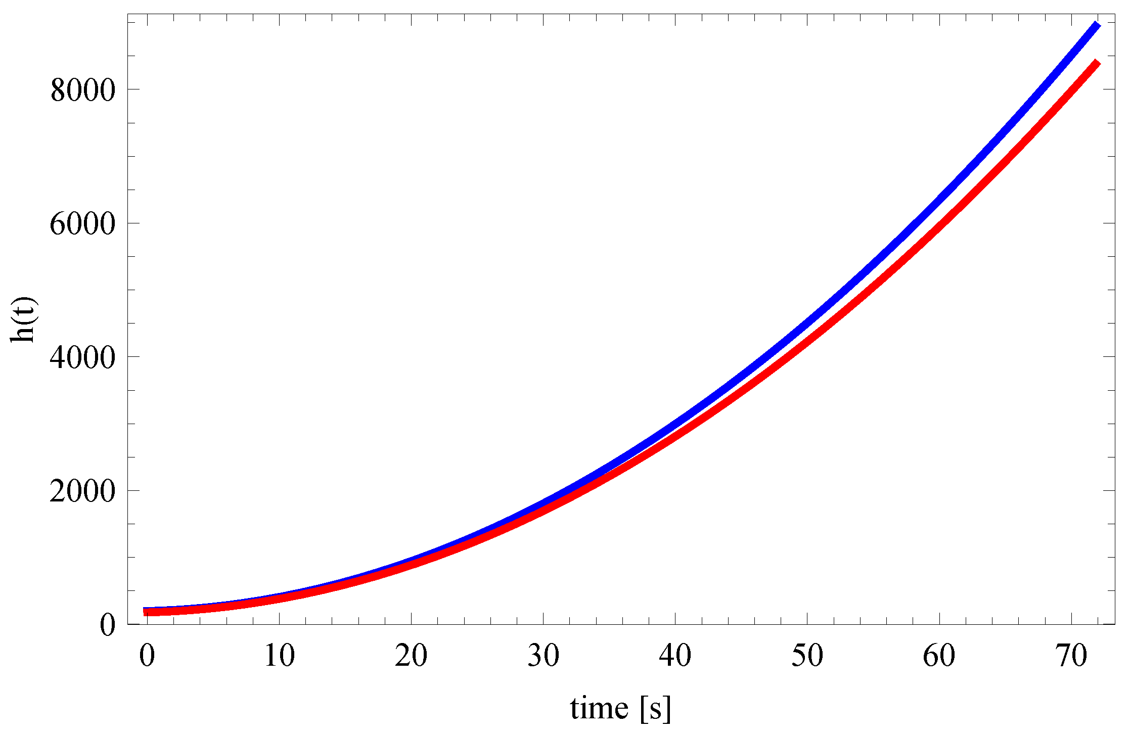
Figure 2.
(a) Measurements of the temperature (black line) and reconstructed temperature (blue line); and (b) distribution of errors for this reconstruction (100 × 1995) .
Figure 2.
(a) Measurements of the temperature (black line) and reconstructed temperature (blue line); and (b) distribution of errors for this reconstruction (100 × 1995) .
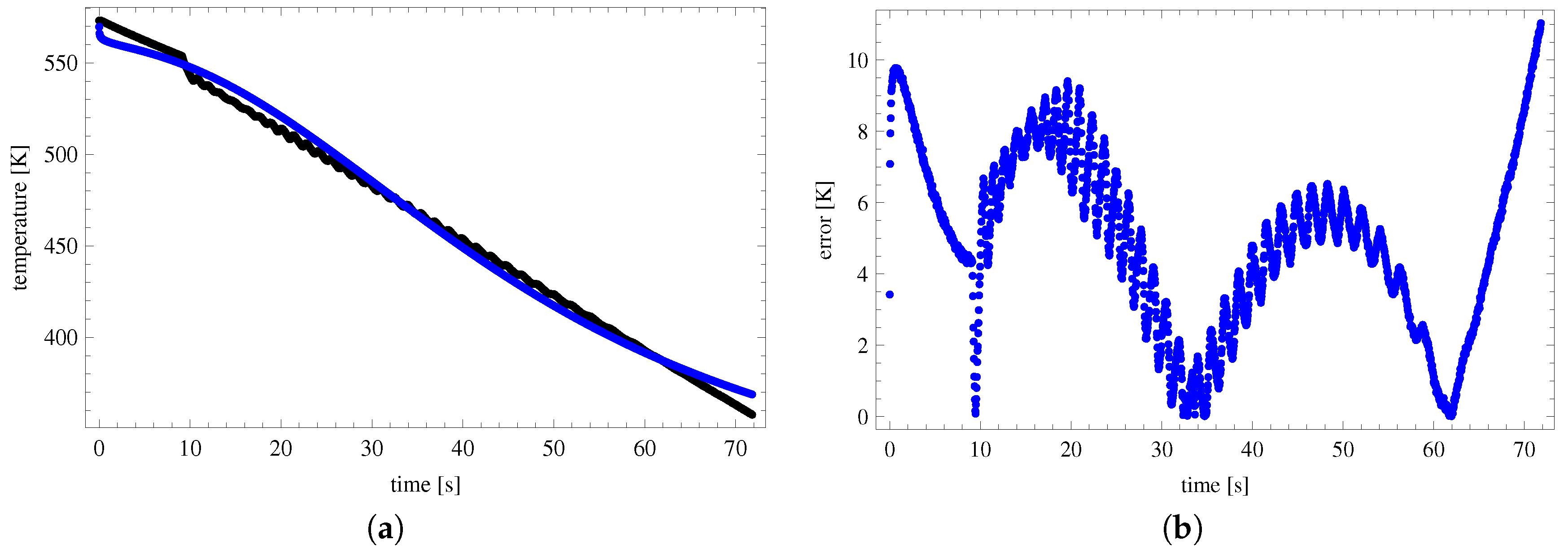
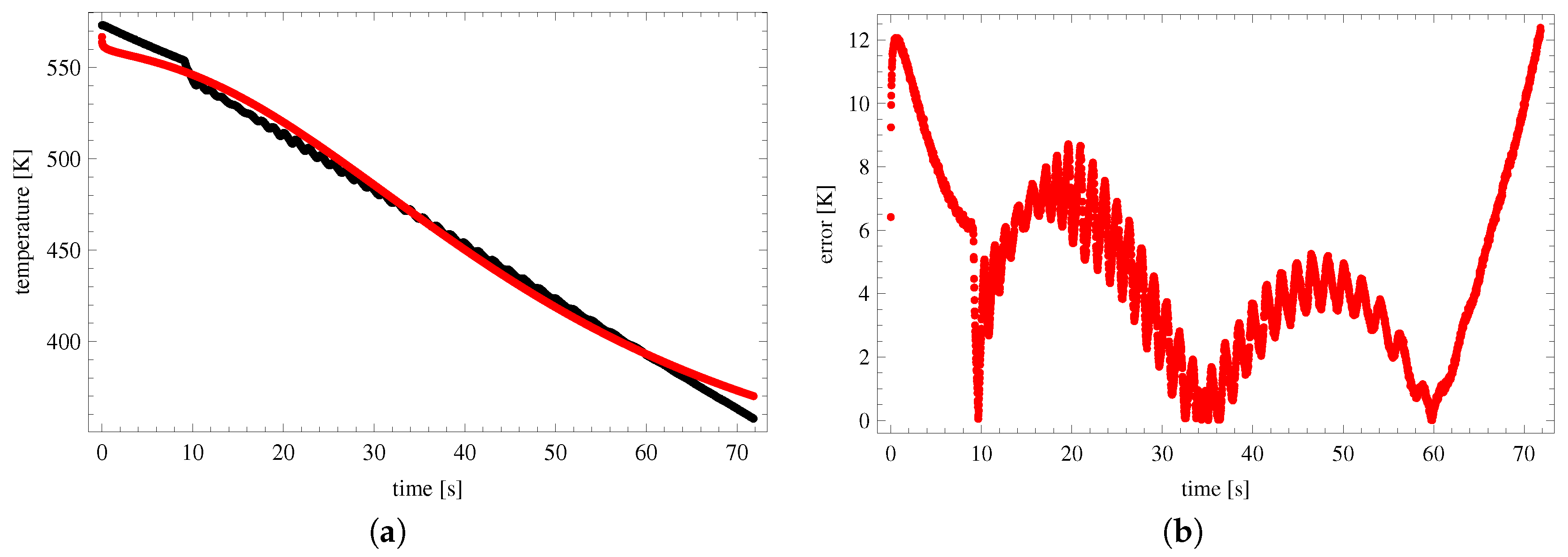
Figure 3.
(a) Measurements of the temperature (black line), reconstructed temperature (red line); and (b) distribution of errors for this reconstruction (100 × 3990).
Figure 3.
(a) Measurements of the temperature (black line), reconstructed temperature (red line); and (b) distribution of errors for this reconstruction (100 × 3990).

Table 1.
Results of calculation for grids 100 × 1995 and 100 × 3990 (—reconstructed value of parameter, —standard deviation ()).
Table 1.
Results of calculation for grids 100 × 1995 and 100 × 3990 (—reconstructed value of parameter, —standard deviation ()).
| 100 × 1995 | 100 × 3990 | |||
|---|---|---|---|---|
| 300.00 | 69.74 | 237.91 | 67.78 | |
| 569.73 | 2.02 | 566.74 | 3.80 | |
| 1.63 | 0.40 | 1.52 | 2.20 | |
| 4.72 | 0.67 | 5.00 | 4.27 | |
| 198.02 | 46.05 | 178.05 | 51.73 | |
| 0.20 | 0.05 | 0.21 | 0.09 | |
| value of the functional | 246.98 | 352.88 | ||
Table 2.
Errors of temperature reconstruction in measurement point for grids 100 × 1995 and 100 × 3990 (—average absolute error, —maximal absolute error, —average relative error, —maximal relative error).
Table 2.
Errors of temperature reconstruction in measurement point for grids 100 × 1995 and 100 × 3990 (—average absolute error, —maximal absolute error, —average relative error, —maximal relative error).
| 100 × 1995 | 100 × 3990 | |
|---|---|---|
| 4.92 | 4.77 | |
| 11.04 | 12.38 | |
| 1.06 | 1.02 | |
| 3.08 | 3.46 |
© 2017 by the authors. Licensee MDPI, Basel, Switzerland. This article is an open access article distributed under the terms and conditions of the Creative Commons Attribution (CC BY) license (http://creativecommons.org/licenses/by/4.0/).
Share and Cite
MDPI and ACS Style
Brociek, R.; Słota, D.; Król, M.; Matula, G.; Kwaśny, W. Modeling of Heat Distribution in Porous Aluminum Using Fractional Differential Equation. Fractal Fract. 2017, 1, 17. https://doi.org/10.3390/fractalfract1010017
AMA Style
Brociek R, Słota D, Król M, Matula G, Kwaśny W. Modeling of Heat Distribution in Porous Aluminum Using Fractional Differential Equation. Fractal and Fractional. 2017; 1(1):17. https://doi.org/10.3390/fractalfract1010017
Chicago/Turabian StyleBrociek, Rafał, Damian Słota, Mariusz Król, Grzegorz Matula, and Waldemar Kwaśny. 2017. "Modeling of Heat Distribution in Porous Aluminum Using Fractional Differential Equation" Fractal and Fractional 1, no. 1: 17. https://doi.org/10.3390/fractalfract1010017