Development of Framework for Aggregation and Visualization of Three-Dimensional (3D) Spatial Data


1
The Chang School of Continuing Education, Ryerson University, 350 Victoria Street, Toronto, ON M5B 2K3, Canada
2
School of Computing & Information Systems, Athabasca University, 10011, 109 Street, Edmonton, AB T5J 3S8, Canada
3
Faculty of Science and Technology, Athabasca University, 10011, 109 Street, Edmonton, AB T5J 3S8, Canada
*
Author to whom correspondence should be addressed.
Big Data Cogn. Comput. 2018, 2(2), 9; https://doi.org/10.3390/bdcc2020009
Submission received: 17 February 2018
/
Revised: 14 March 2018
/
Accepted: 19 March 2018
/
Published: 21 March 2018
Abstract
:Geospatial information plays an important role in environmental modelling, resource management, business operations, and government policy. However, very little or no commonality between formats of various geospatial data has led to difficulties in utilizing the available geospatial information. These disparate data sources must be aggregated before further extraction and analysis may be performed. The objective of this paper is to develop a framework called PlaniSphere, which aggregates various geospatial datasets, synthesizes raw data, and allows for third party customizations of the software. PlaniSphere uses NASA World Wind to access remote data and map servers using Web Map Service (WMS) as the underlying protocol that supports service-oriented architecture (SOA). The results show that PlaniSphere can aggregate and parses files that reside in local storage and conforms to the following formats: GeoTIFF, ESRI shape files, and KML. Spatial data retrieved using WMS from the Internet can create geospatial data sets (map data) from multiple sources, regardless of who the data providers are. The plug-in function of this framework can be expanded for wider uses, such as aggregating and fusing geospatial data from different data sources, by providing customizations to serve future uses, which the capacity of the commercial ESRI ArcGIS software is limited to add libraries and tools due to its closed-source architectures and proprietary data structures. Analysis and increasing availability of geo-referenced data may provide an effective way to manage spatial information by using large-scale storage, multidimensional data management, and Online Analytical Processing (OLAP) capabilities in one system.
1. Introduction
Recent developments in remote sensing data, monitoring networks, and geographic information systems (GIS), like movements of open access and open data lead to the unprecedented growth of data [1,2,3]. There currently exist many large repositories and cloud storage of analytical and subject-oriented databases, such as national censuses, statistical frameworks of the UN System of Environmental-Economic Accounting [4,5,6,7,8,9,10]. Big Data technologies together with cloud computing create new opportunities for data intensive research and massive data processing from earth remote sensing in a multi-disciplinary environmental domain. Sustainable development requires multidisciplinary approaches to process Big Data, including climate change, environmental health, water resources, land use and land cover, web technologies, digital earth, and so on [8,9,10]. This also requires dealing with big data complexity, such as large scale, structured and unstructured data, online and real-time interaction and processing, cross formats, and so on [9,10,11,12]. This makes data management and processing very difficult using conventional methods in a reasonable time although big data offers an environment rich information and opportunities to explore the data in more precise ways. It is still challenging how to process such big amount of data to extract useful information of economic and environmental sustainability because of complexity of the big data obtained from various sources and scales.
Several recent studies focus on using big data and cloud computing techniques in environmental data analysis. Lokers et al. [8] presented a theoretical framework to analyze data-intensive cases related to big data usage in agro-environmental domain. This research indicates that data-intensive research evolves around capturing huge heterogeneity of interdisciplinary data and around creating trust between data providers and data users. Votolo et al. [9] gave an overview of currently available implementations that are related to web-based technologies for processing large and heterogeneous datasets and discuss their relevance within the context of environmental data processing, simulation, and prediction. Cavallaroa et al. [13] presented how big data analytics take advantages of techniques from the fields of data mining, machine learning, or statistics, with a focus on analyzing big data in remote sensing with modern technologies. Kussul et al. [14] proposed a framework for solving the large-scale classification and area estimation problems in the remote sensing domain based on deep learning. In this framework, self-organizing maps, multi-layer perceptron, and geospatial analysis were used for segmentation, classification and fusion, and for some post-processing, respectively. Wolfert et al. [10] presented a review on how big data is being used to provide predictive insights in farming operations, drive real-time operational decisions, and redesign business processes for game-changing business models. The authors of this paper believe that the big data will cause major shifts in roles and power relations among different players in the current food supply chain networks. Yang et al. [15] investigated how cloud computing can be used to address big data challenges, especially in climate studies, geospatial knowledge mining, land cover simulation, and dust storm modelling. Fritz et al. [16] described the global land cover and land use reference data derived from the Geo-Wiki crowdsourcing platform. These global datasets provide information on human impact, land cover disagreement, wilderness, and land cover and land use.
Geospatial and environmental data include not only maps of locations of land usage, but also multiple attributes, such as socioeconomic data extracted from state and national census, and this is also a type of big data. These data sets are heterogeneous across various data sources and their file formats are inconsistent, since different suppliers tend to use proprietary data and file formats. They may have static or dynamic characteristics. Thus, there may be little or no commonality between formats used. This has led to increased challenges in capturing and analyzing such spatial data.
Advancements in computing, visualization, and Internet technologies [17,18,19,20] have allowed two-dimensional (2D) and three-dimensional (3D) images to aggregate map layers into one graphical representation. Aggregation of different data sources can generate a new map with higher levels of informational detail that is not possible by any of the individual systems [18]. By sharing and aggregating this information over the Internet, enhanced accessibility and time responses can effectively improve the interpretation of used information/data sources when compared to conventional distribution of maps or character based online systems [21]. Aside from environmental modelling, using maps to visualize data can enable better interpretation of complex geographical data [22], identify patterns, and help in planning resource distribution for policy and decision making [23]. Soulard et al. [24] reported the harmonization of forest disturbance datasets using multiple data sources. Villarreal et al. [25] used three vegetation land cover maps from different geographic scales to improve the accuracy of wildlife habitat models. Therefore, aggregating, in the environment and resource management, provides a visual assessment for investigating spatial distribution of agricultural and forest production and pollution diffusion, with potential associations and their underlying causes [26] and can help the calibrations and classifications of land uses from remote sensing images. The accurate modelling of spatial data requires the definition of two kinds of metadata: (a) warehoused metadata that models data structures and maintains integrated data from multiple data sources, and (b) aggregation metadata that specifies how the warehoused data should be aggregated to meet analysis needs of decision makers.
New mapping technologies, such as Google Earth, offer free satellite and aerial photos of most of the Earth’s land surface, which has led to an increased uptake in mapping technology for uses that are relevant to environmental health [27,28,29,30,31]. Xiong et al. [30] developed an automated cropland mapping of algorithms to aggregate continental Africa using Google Earth Engine cloud computing. Google Earth Engine cloud computing is now providing a platform for data production and analysis using Python and JavaScrip [31]. However, Google Earth does not allow for user customization because it provides no external plug-in infrastructure. Developments in GIS have made mapping of spatial data more commonplace and is being used in a wide range of applications. Current commercial GIS vendors use closed-source architectures and proprietary data structures, limiting their ability to add libraries and tools, including those for transient watershed modelling, and limiting geospatial data to their own preferred sources. The vendor ESRI, through its ArcGIS platform [32], for example, creates a GIS infrastructure that provides users with servers, clients, and geospatial data. However, ArcGIS does not provide a plug-in functionality for the use of aggregating and fusing geospatial data from different data sources. Because of large scale of data, some formats cannot be treated in ArcGIS. Therefore, it is desirable to provide a plug-in infrastructure that allows users to perform their own customization. If multiple map services for the same geographical region could be aggregated, the resulting map produced would include more spatial information. Therefore, the aggregation and fusion of spatial data in GIS is a useful feature in the environmental sciences, although this only marginally presents in current commercial GIS, primarily through ad-hoc solutions [33,34,35]. The successful use of this data depends to a large extent on the user’s ability to access, integrate, and analyze the data [36,37,38].
The objective of this paper is to develop a framework called PlaniSphere [39] for the aggregation and visualization of various map sources. It allows for synthesizing raw data of geometric components and aggregate non-spatial information contained in a data warehouse associated to those components, defined in GIS fact tables. Aggregation of map data can produce new fusion maps with a higher level of detail than what is currently available.
2. Methodology
2.1. Conceptual Model of Data Aggregations
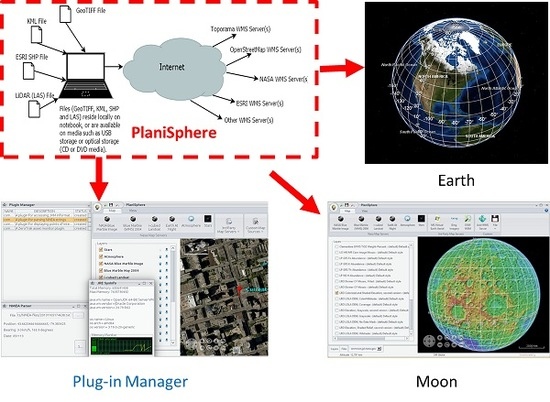
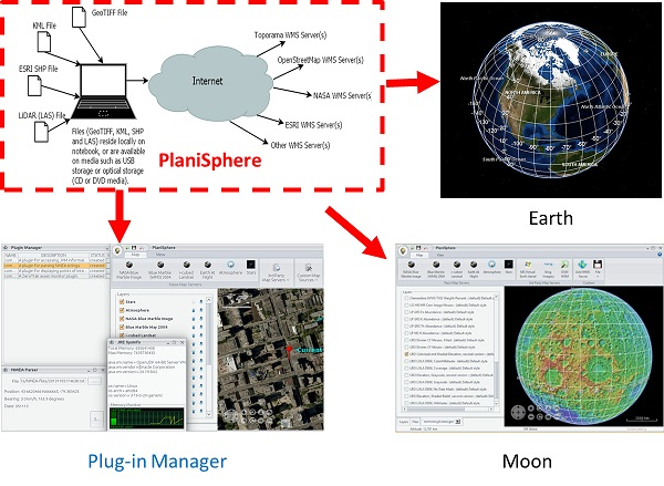
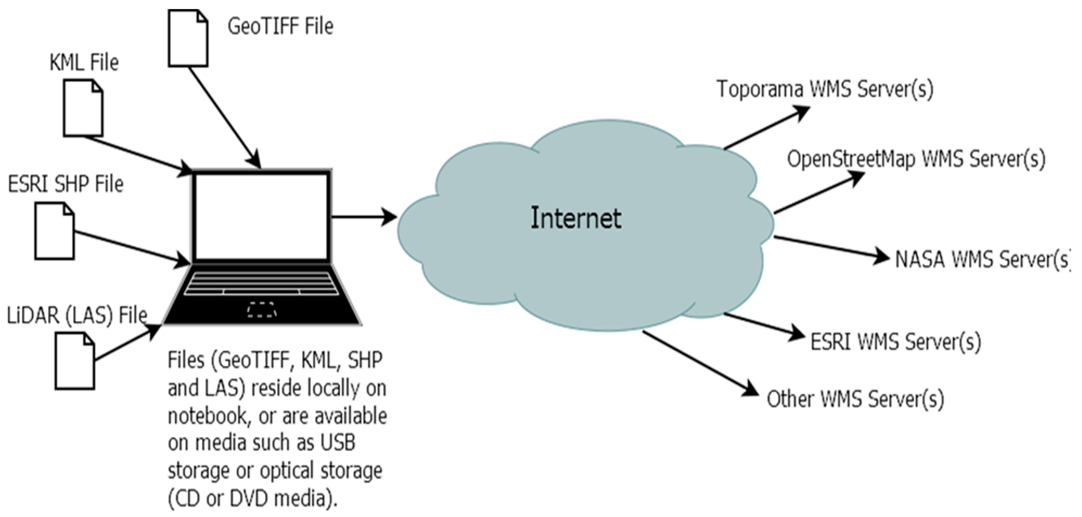
A software tool that aggregates and fuses various geospatial data sources needs to reconcile differences from multiple data formats and service providers. Alternatives to commercial vendors are open-source suppliers, but existing open-source suppliers, such as GeoServer [40] and MapServer [41], provide fragmented solutions for geospatial data, services, and infrastructure. Usually, these open-source projects are independent of each other, although GeoServer and MapServer will allow for clients to connect using a Web Map Service (WMS) protocol [42] from the OpenGeospatial Consortium (OGC) [34,43]. Techniques for performing complex analysis of information stored in a data and map warehouse has been developed, including such systems as the OGC [34,43] and Online Analytical Processing (OLAP) [35,44,45]. This provides specifications of interoperability among vendors [28,29]. The software tools that this project creates will facilitate the usage of various geospatial data, regardless of their format and location. Figure 1 provides a high-level overview of the proposed solution that is implemented in this project. Geospatial data can be provided from local storage or from remote servers through the Internet using WMS. The software tool can aggregate files from local storage that conforms to widely used file formats, such as: GeoTIFF files, ESRI shape files, KML, GeoJSON, and LASer files (Figure 1).
The level of integration required would be high and may be beyond the capabilities of open-source suppliers. WMS and WFS have been created to aid in transferring geospatial data over the Internet in PlaniSphere. The design of modern map servers, such as GeoServer and MapServer, is based on service-oriented architecture (SOA). NASA World Wind [46] can access remote map servers using WMS version 1.3, and also parses files that reside in local storage and conforms to the following formats: GeoTIFF, ESRI shape files, and Keyhole Markup Language (KML). WMS is used as the underlying protocol that supports SOA. Also, WMS supports the interoperability between map servers and clients. The end result of WMS is to produce a map that is represented by an image stored as a png, gif or jpg format [47]. These analyzing techniques and the increasing availability of geo-referenced data facilitates an effective way to manage spatial information by providing large-scale storage, multidimensional data management, and OLAP querying capabilities, together in one system [48,49,50]. WMS is a standard widely used for accessing and retrieving maps from remote servers made available over the Internet. WMS can be used to retrieve maps from public and private servers via the Internet. WMS versions 1.1 and 1.3 are widely supported by commercial vendors and open-source suppliers, but WMS version 1.3 is not backwards compatible with WMS version 1.1 [42]. WMS can retrieve geospatial data from a remote server without knowing the originating file(s) and their type(s)/format(s), but it requires a server-side implementation. When a user retrieves geospatial data from local storage, they may not have a server-side implementation of WMS, and, as a result, WMS cannot be used.
2.2. Graphic User Interface Design
PlaniSphere is a desktop application with graphical capabilities. Its functionality is available to the user through a graphical user interface (GUI) (Figure 2). Because the NASA World Wind API [46] lacks export capabilities and a plug-in infrastructure, the functionality and design of the GUI for PlaniSphere is extremely important. It uses a similar GUI design as MS Office 2007 and newer applications. At the heart of the plug-in infrastructure is the Plug-In Manager (Figure 3).
PlaniSphere revolves around a main window with a ribbon toolbar. The toolbar presents the core features to the user. Under the ribbon, there is a working area where a map or 3D virtual globe image is displayed. The optional capability to manipulate any layers within the map is in a tabbed pane to the left of the working area. See Figure 2 for the general layout of the main window.
The ribbon toolbar in PlaniSphere allows for users to load any resources available from any map servers that support the WMS 1.3 protocol. PlaniSphere can connect to multiple servers provided the URL of the server is known. The software loads any geospatial data resource represented by files, such as an ESRI shape file, GeoTIFF, and KML. Each file represents a single layer that can be rendered on the map. A ribbon band is dedicated to “Custom Map Sources” support. It should be noted that each time a connection to a known map server is required the user needs to click on the “Add WMS Server” button in the ribbon band. Each file type is then represented by a button.
PlaniSphere is built from the ground up and possesses several advantages over existing GIS packages. Thus, PlaniSphere supports many well-known open standards, such as WMS, WFS, and file formats (KML, GeoTIFF, GeoJSON, LAS, and ESRI Shape Files). Table 1 lists basic files and data sources that are provided by PlaniSphere. The second advantage is that PlaniSphere is platform independent. It is implemented in Java and runs on any desktop (Linux, macOS, MS Windows) that supports Java version 8 or higher. The third advantage is that PlaniSphere renders GIS data using the World Geodetic System 1984 (WGS 84) with projections (Round/Spherical, Mercator, Flat-Modified Sinusoidal).
2.3. Implementation
PlaniSphere allows for users to build their own applications by providing a geographic rendering engine for powering a wide range of projects, from satellite tracking systems to traffic simulators. PlaniSphere is designed for interoperability. It consumes and renders data from any major spatial data source using open standards. Using GeoServer becomes an easy method of connecting existing information and data to virtual globes, such as Earth and NASA World Wind as well as to web-based maps, such as OpenLayers, OSM, Google Maps, and Bing Maps. GeoServer functions as the reference implementation of the Open Geospatial Consortium Web Feature Service standard. WMS and WFS are used as standard protocol for serving (over the Internet) georeferenced map images that a map server generates using data from a GIS database and also implements the Web Coverage Service and Web Processing Service specifications. PlaniSphere will aggregate various map services, as WMS and WFS are a standard that is widely used for accessing maps from various servers and can be used to retrieve maps from public and private servers that are available over the Internet. Geospatial information that resides on local storage (GeoTiff, ESRI shape files, KML files, las files, etc.) may also be used (Figure 1). A 3D virtual globe desktop application that provides a rich set of features for displaying and interacting with geospatial data is created based on NASA WorldWind for Java.
The 3D virtual globe has the following characteristics:
- a Java SE 1.8 application that can run on any operating system;
- the 3D virtual globe is an interactive application that has a low learning curve;
- open-standard interfaces to GIS services and databases
- capable of rendering in 3D/2D: ESRI shapefiles, GeoTIFF, KML, LiDAR;
- a plugin framework that can be used to expand PlaniSphere by any third party (Figure 4); and,
- capable of rendering in 3D/2D high-resolution imagery, terrain and geospatial information from any source using WMS 1.3.
Each geospatial data source (WMS endpoint or ESRI shapefile, GeoTIFF and KML file) creates its own appropriate layer. A layer is a direct or indirect instance of RenderableLayer or TiledImageLayer types.
The algorithm is useful in aggregating geospatial data of a graphical nature. The files that compose the geospatial data are maps or content that can be converted into an image. GeoTIFFs are images with geotags; ESRI shapefiles are simplified 2D maps; KML files are XML files that contain information that can be drawn on top of a map. Algorithm 1 may be used interactively by a user in their viewing session. The user can select in real time the area of interest and the layers to be aggregated. The resulting image is generated almost in real time. The user may interactively reorder the layers as needed. Each time the layers are reordered, a new image is generated. Figure 5 exhibits an example of aggregating layers in a viewing session. Out of all the layers that are available, only two are visible and used in the aggregation. Only visible layers are aggregated using this algorithm by PlaniSphere. The two visible layers that are involved in the aggregation and fusion are “Bing imagery” and “planet_osm_line”. “Bing imagery” is a base layer, while “planet_osm_line” is an overlay layer.
| Algorithm 1: Algorithm for Graphical Aggregation and Fusion of Geospatial Data refers to Java and NASA World Wind Types such as RenderableLayer, TiledImageLayer, etc. [46,51]. |
|
3. Results and Discussion
As a multi-function platform, PlaniSphere is well supported by data management software such as databases and GIS platforms through the NASA World Wind API framework and is compatible with the OGCs and WMS. Unlike Google Earth, Planisphere provides a plug-in function for users to build their own applications. Therefore, it can aggregate data and metadata in one single file using a text format. Plug-in window function allows for users to develop further self-describing data formats for storage, transfer and aggregation of 3D spatial data and metadata information using JavaScript on demand. Online web data processing unusually allows for utilizing with one or several datasets in different formats, which are assessible locally or online for user interaction and create a web app. This enables interacting and interchanging data with several datasets in different data formats, including plain text, markup languages and binary files and to easily create interactive visualization of 3D globe, map and conventional descriptions of geographical features, vector, coverages, and sensor data. By using KML, the semantic meaning of the data can be extracted from the file itself making it suitable to optimally represent the metadata. The platform enables visualization and mapping of 3D spatial data and interactive mapping applications, such as hovering over a graph, zoom in/out on a particular portion of a map/graph through MapServer and GeoServer. Thus, PlaniSphere may be used for simple purposes, such as identifying camp sites and bicycle paths, and for more complicated purposes, such as vehicle tracking and monitoring weather patterns. The following illustrates PlaniSphere using five examples of landscape and environmental applications that are being studied and/or researched:
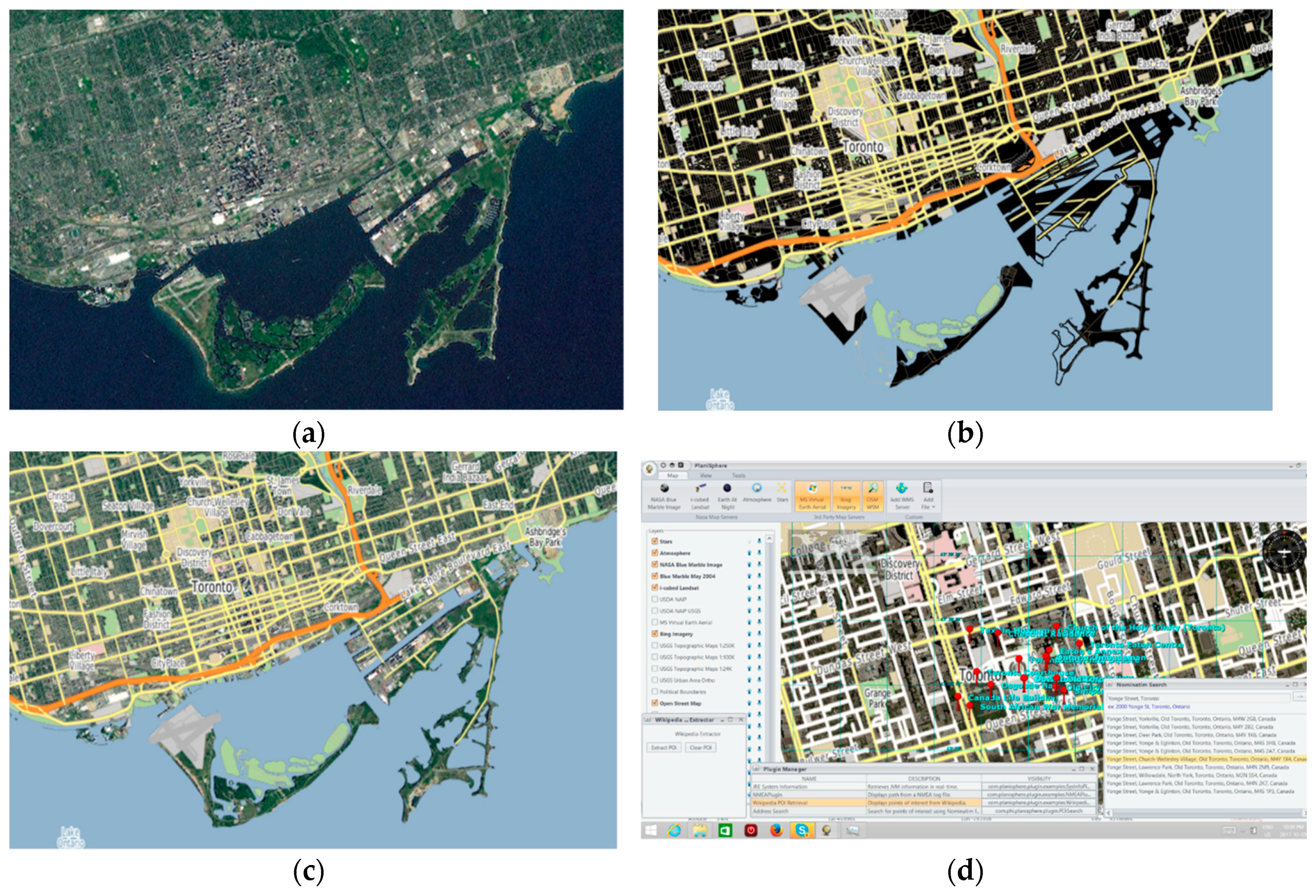
Figure 4 shows a fusion of multiple layers from different WMS servers. First, Bing Map provides a background layer using a LandSat 7 image with buildings and landscape details (Figure 4a). An OpenStreetMap (OSM) of the same area with roads and names WMS layer represents the road network that was used for the second layer (Figure 4b) and it can be easily updated. The geospatial data used in Figure 4a (LandSat) and Figure 4b (Open Street Map) are provided by two independent and distinct sources from NASA and a community of mappers, respectively. Then, the user can generate an enhanced map of the same area containing all of the details from the Figure 4a,b (buildings, landscape, roads, and names). The aggregation and fusion of the photograph and the road map is the rendered result, as depicted in Figure 4c. The third layer is metadata from Wikipedia, which provides a rest web service [52], where points of interest may be retrieved for an area of interest. In this case, the area of interest is a neighborhood in downtown Toronto. Wikipedia provides spatial data using the Wikipedia GeoData extension [52], which is a proprietary standard. A plugin was created to consume such a proprietary standard. This plugin is the Wikipedia Plugin Extractor, which is exhibited at the bottom left of Figure 4d. This is a unique demonstration of aggregation of map data of different map formats. As far as OGC compliance concerns, the WMS services have made the OSM maps one of the many layers in the employed GIS application. Thus, the multiplicity of layers in WMS allows for the user to focus on the required one (e.g., buildings, names, or transportation here). In terms of the data adaptation, OSM data is projected in Toronto transport Grid so it can be easily integrated to the rest of the map sources in the system, either in raster or in vector.A PlaniSphere Plug-in, demonstrating OLAP capabilities by identifying boundaries of municipalities based on concentrations of points of interest (Figure 5). Municipality boundaries may be determined by the absence of points of interest. Note that the blue border represents the extrapolated boundary of the municipality. The OLAP plugin uses two factors to identify areas of high population concentration. The first factor is the number of points of interest retrieved per square kilometer. The second factor is the distance between points of interest within the square kilometer in question. The higher the number of points of interest, the closer the distance between neighboring points and the higher the population concentration of the area. Using the OLAP process, areas of lower concentration can be identified in Figure 5. OLAP enables the end-users to perform other ad hoc analysis of data in multiple dimensions, through Plugin Function, such as LULC [53], thereby providing the insight and understanding that they need for better decision-making.
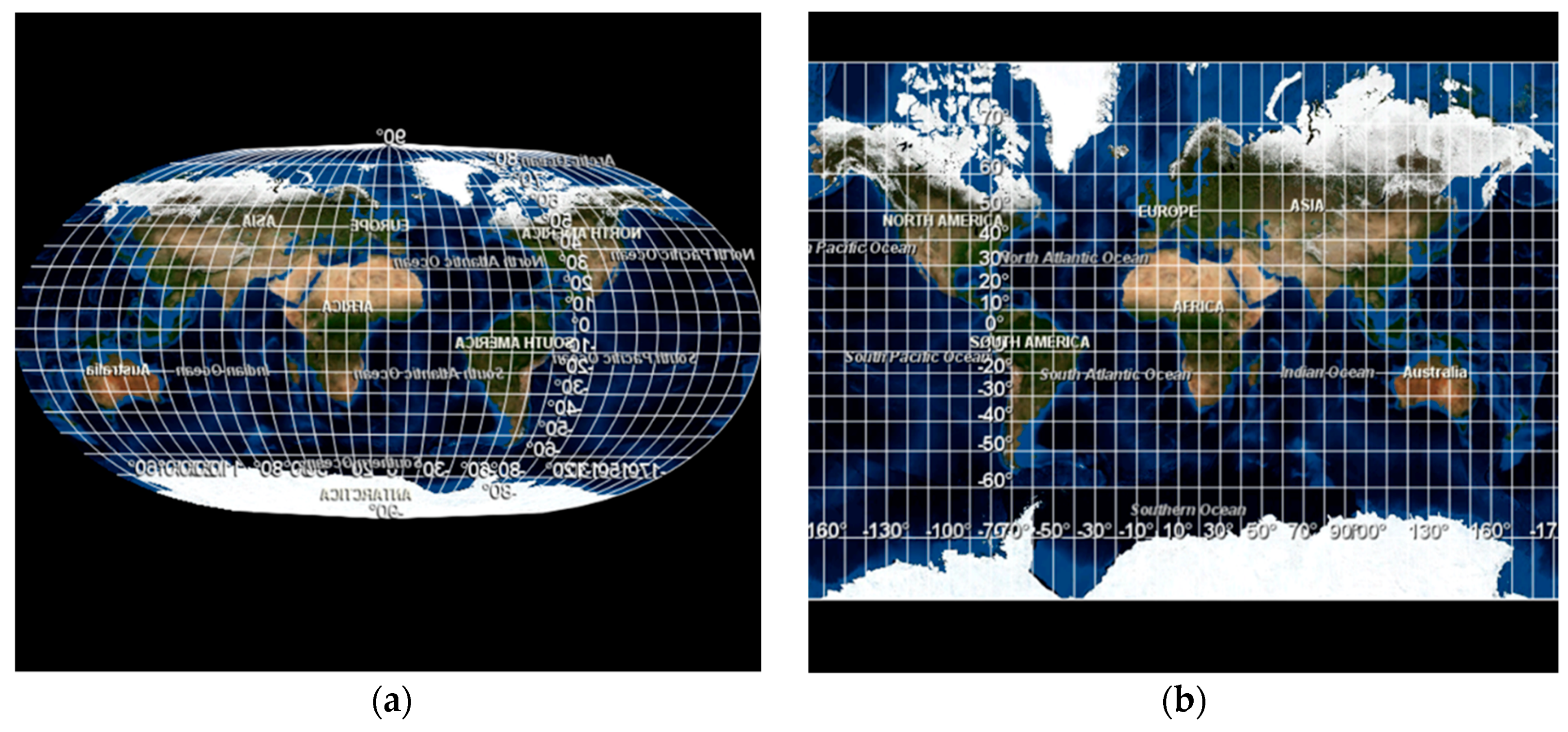
When map data of other planetary bodies exists from Jet Propulsion Laboratory and is available by standard mechanisms, such as WMS, PlaniSphere may consume these maps and render them. Figure 6a,b exhibit map data of our earth, while Figure 6c,d render an overview of the Moon. It was created by a single layer from the Jet Propulsion Laboratory WMS server. Figure 6a,b show the Blue Marble Next Generation imagery from NASA WMS. It should be noted that each figure renders a map imagery using a different projection. Although all of the figures render the same map imagery, Figure 6a renders Blue Marble Next Generation imagery displayed using Flat-Modified Sinusoidal Projection and Figure 6b renders Blue Marble Next Generation imagery displayed using the Mercator Projection. Figure 6c shows a moon. In Figure 6d, several detail points of interest of the Moon are exhibited. This image is composed of a Clementine Elevation map and a superimposed Lunar Nomenclature layer. Both of the map layers are made available from the Jet Propulsion Laboratory WMS and use the same WMS server and layers for rendering imagery.
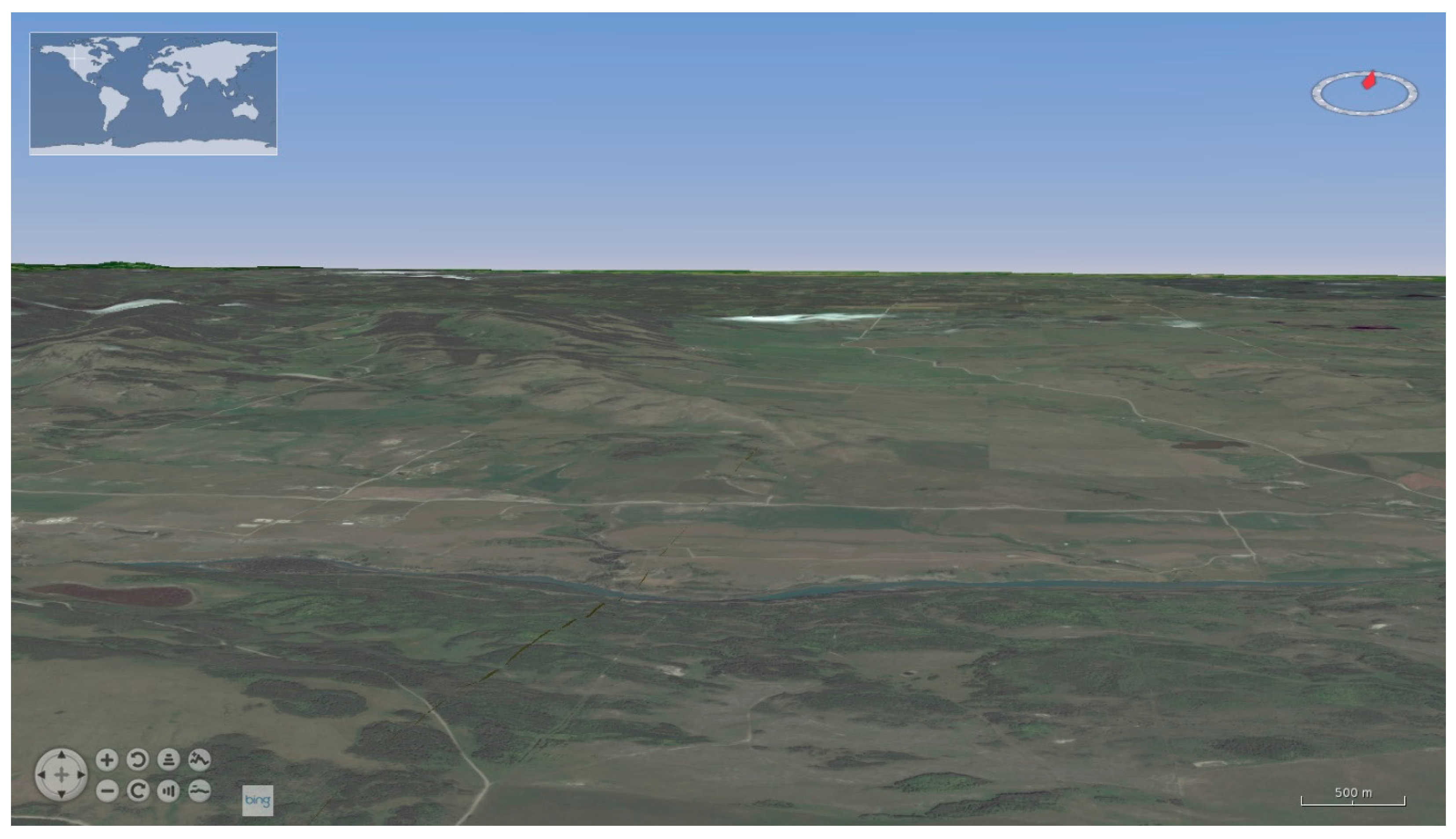
Figure 7 shows the capability of aggregating 2D maps into a 3D geospatial data set. The background is created by using Bing Aerial photographs with a resolution of 30 m and is projected on a 3D space with the aid of the Shuttle Radar Topography Mission (SRTM) elevation data [54]. The foreground shows LiDAR [55] cloud points of a neighborhood in North Vancouver. Figure 8 shows a 3D visualization with some hills and farm land superimposed over a Bing aerial 2D landscape map and data at an area near Cochrane, Alberta (51.1830, −114.4742). A LandSat photograph with landscape details and an elevation map of the same area are provided by two independent and distinct sources. The end result is the aggregation and the fusion of the photograph and the landscape map.
Geospatial information plays an important role in environmental modelling, resource management, business operations, government policy, and in enhancing the quality of life. Currently, there is a greater quantity of geospatial information available from remote sensing, monitoring networks, survey, and censuses than in any time in history. However, difficulties arise from the fact that there may be little or no commonality between the formats of these geospatial databases at the spatial and temporal scales. Image information and quality with respect to land cover patches of varying sizes and shapes are determined by its spatial resolution and the image processing used. Most multiscale approaches use labels from only one level of the categorical scale, i.e., they are categorically monoscale. A patch can be labeled as general class only when, at a certain spatial scale, it is judged to contain sufficient information likely to correspond to patches of more than one specific class. The term “categorical scale” (also called categorical resolution by other authors) refers to the level of detail in the categories used in classification.
In order to utilize different data for any new and innovative applications, many disparate data sources must be aggregated to make use of the large body of geospatial information available. However, some visualization tools, such as Google map, have no functions for users to perform their own modelling and data aggregation. Unlike Google map, PlaniSphere provides plug-in functionality, which allows for users to analyze and fuse spatial data through modelling algorithms. The plugin functionality of the system shows that this platform can be adapted for different applications, such as environmental spatial analysis or distance education. This topic is of interests in the scope and priority of Information Visualization. For example, as large-scale measurements are time-consuming and costly, many projects are restricted to single point or local data available for the RS model calibration. As a result, land classification from remote sensing images can be difficult because of lack of data for model calibration. In the plugin window, a remote sensing (RS) image of LULC can be classified through its colour bands [53]. The image of RS raw data was stored as the coordinate of each point post-processed to produce several per-point attributes, including the elevation, RGB color, and classification codes of the point. The latter are used to label points as belonging to buildings, bare earth, crops, water, etc. Further post-processing allowed for comparing with its category of national census data in this region, typically involving the integration of other data format, such as census data. The national census data was used for validation and calibration of classification of LULC of remote sensing. Classification of LULC of remote sensing image can be performed in regional scale since many censuses are available at the national scale. This provided an approach to improve the accuracy of LULC classifications using conventional approaches of limited field labeling and sampling at small scale. Therefore, PaniSphere provides not only a visualization platform, but also an analyzed window for various users.
4. Conclusions
A platform framework named PlaniSphere has been developed for the aggregation and fusion of various geospatial data and raw data. The framework uses NASA World Wind to access remote map servers using WMS. WMS has been used to aid in transferring geospatial data over the Internet as the underlying protocol that supports service-oriented architecture (SOA). We have illustrated the potential applications for the PlaniSphere platform in aggregation of 2D spatial data and maps into 3D visualization using six examples of open street maps, earth, moon, and land landscape with hills and farmland. The results show that PlaniSphere can aggregate and parses files that reside in local storage and conforms to the following formats: GeoTIFF, ESRI shape files, KML, GeoJSON, and LiDAR(LASer). Internet spatial data can create geospatial data sets (map data) from multiple sources regardless of who the data providers are. These analyzing techniques and the increasing availability of geo-referenced data, could provide an effective way to manage spatial information by providing large-scale storage, multidimensional data management and OLAP querying capabilities together in one system. Because of the rich data resource with various data formats, this can offer a new approach for remote sensing map aggregation. The plug-in function of this framework illustrates that the platform can be expanded for greater uses, such as special data formats in environmental spatial analysis and distance education by providing customizations to serve future uses, which existing GIS software is not available. Aggregation of different data sources will generate a new map with a higher level of informational detail that is not currently provided by any individual vendors.
Acknowledgments
Mihal Miu would like to thank James R. Miller, Department of Electrical Engineering and Computer Science, The University of Kansas for providing access to Lidar Data Visual Analysis and Editing. http://people.eecs.ku.edu/~miller/; M.M. would like to thank the City of Vancouver for LiDAR data collected in 2013 with coverage up to extents of City of Vancouver’s legal jurisdiction. http://data.vancouver.ca/datacatalogue/LiDAR2013.htm.
Author Contributions
Mihal Miu developed idea and software, implemented the program and paper writing; Xiaokun Zhang involved in drafting or critically revisiting the manuscript; M. Ali Akeber Dewan involved in data acquisition, image processing and critically revisiting; Junye Wang developed concept, interpreted the results and structured the manuscript. All authors have read and approved the final manuscript.
Conflicts of Interest
The authors declare no conflict of interest.
References
- Chi, M.; Plaza, A.; Benediktsson, J.A.; Sun, Z.; Shen, J.; Zhu, Y. Big Data for Remote Sensing: Challenges and Opportunities. Proc. IEEE 2016, 104, 2207–2219. [Google Scholar] [CrossRef]
- Ma, Y.; Wang, L.; Liu, P.; Ranjan, R. Towards building a data-intensive index for big data computing—A case study of Remote Sensing data processing. Inf. Sci. 2015, 319, 171–188. [Google Scholar] [CrossRef]
- Guo, H.; Wang, L.; Chen, F.; Liang, D. Scientific big data and Digital Earth. Chin. Sci. Bull. 2014, 59, 5066–5073. [Google Scholar] [CrossRef]
- Yu, L.; Liang, L.; Wang, J.; Zhao, Y.; Cheng, Q.; Hu, L.; Liu, S.; Yu, L.; Wang, X.; Zhu, P.; et al. Meta-discoveries from a synthesis of satellite-based land-cover mapping research. Int. J. Remote Sens. 2014, 35, 4573–4588. [Google Scholar] [CrossRef]
- United Nations; European Commission; Food and Agriculture Organization of the United Nations; International Monetary Fund; Organisation for Economic Cooperation and Development; World Bank. System of Environmental-Economic Accounting 2012: Central Framework, Prepublication (White Cover). Available online: http://unstats.un.org/unsd/envaccounting/White_cover.pdf (accessed on 28 January 2018).
- Wang, J.; Cardenas, L.M.; Misselbrook, T.H.; Gilhespy, S. Development and application of a detailed inventory framework of nitrous oxide and methane emissions from agriculture. Atmos. Environ. 2011, 45, 1454–1463. [Google Scholar] [CrossRef]
- Shrestha, N.K.; Du, X.; Wang, J. Assessing climate change impacts on fresh water resources of the Athabasca River Basin. Sci. Total Environ. 2017, 601–602, 425–440. [Google Scholar] [CrossRef] [PubMed]
- Lokers, R.; Knapen, R.; Janssen, S.; van Randen, Y.; Jansen, J. Analysis of Big Data technologies for use in agro-environmental science. Environ. Model. Softw. 2016, 84, 494–504. [Google Scholar] [CrossRef]
- Vitolo, C.; Elkhatib, Y.; Reusser, D.; Macleod, C.J.A.; Buytaert, W. Web technologies for environmental Big Data. Environ. Model. Softw. 2015, 63, 185–198. [Google Scholar] [CrossRef] [Green Version]
- Wolfert, S.; Ge, L.; Verdouwa, C.; Bogaardt, M.-J. Big Data in Smart Farming—A review. Agric. Syst. 2017, 153, 69–80. [Google Scholar] [CrossRef]
- Daniel, B.K. Reimaging Research Methodology as Data Science. Big Data Cogn. Comput. 2018, 2, 4. [Google Scholar] [CrossRef]
- Hogland, J.; Anderson, N. Function Modeling Improves the Efficiency of Spatial Modeling Using Big Data from Remote Sensing. Big Data Cogn. Comput. 2017, 1, 3. [Google Scholar] [CrossRef]
- Cavallaroa, G.; Riedel, M.; Bodenstein, C.; Glock, P.; Richerzhagen, M.; Goetz, M.; Benediktsson, J.A. Scalable developments for big data analytics in remote sensing. In Proceedings of the IEEE International Geoscience and Remote Sensing Symposium, Milan, Italy, 26–31 July 2015. [Google Scholar]
- Kussul, N.; Shelestov, A.; Lavreniuk, M.; Butko, I.; Skakun, S. Deep learning approach for large scale land cover mapping based on remote sensing data fusion. In Proceedings of the IEEE International Geoscience and Remote Sensing Symposium, Beijing, China, 26–31 July 2016. [Google Scholar]
- Yang, C.; Yu, M.; Hu, F.; Jiang, Y.; Li, Y. Utilizing cloud computing to address big geospatial data challenges. Comput. Environ. Urban Syst. 2017, 61, 120–128. [Google Scholar] [CrossRef]
- Fritz, S.; See, L.; Perger, C.; McCallum, I.; Schill, C.; Schepaschenko, D.; Duerauer, M.; Karner, M.; Dresel, C.; Laso-Bayas, J.-C.; et al. A global dataset of crowdsourced land cover and land use reference data. Sci. Data 2017, 4, 170075. [Google Scholar] [CrossRef] [PubMed]
- Li, J. Assessing spatial predictive models in the environmental sciences: Accuracy measures, data variation and variance explained. Environ. Model Softw. 2016, 80, 1–8. [Google Scholar] [CrossRef]
- Granell, C.; Havlik, D.; Schade, S.; Sabeur, Z.; Delaney, C.; Pielorz, J.; Usländer, T.; Mazzetti, P.; Schleidt, K.; Kobernus, M.; et al. Future Internet technologies for environmental applications. Environ. Model Softw. 2015, 78, 1–15. [Google Scholar] [CrossRef]
- Kuhn, M.; Johnson, K. Applied Predictive Modeling; Springer: New York, NY, USA, 2013. [Google Scholar]
- Shrestha, N.K.; Wang, J. Predicting sediment yield and transport dynamics of a cold climate region watershed in changing climate. Sci. Total Environ. 2018, 625, 1030–1045. [Google Scholar] [CrossRef]
- Maas-Hebner, K.G.; Harte, M.J.; Molina, N.; Hughes, R.M.; Schreck, C.; Yeakley, J.A. Combining and aggregating environmental data for status and trend assessments: Challenges and approaches. Environ. Monit. Assess. 2015, 187, 278. [Google Scholar] [CrossRef] [PubMed]
- Elliott, P.; Wartenberg, D. Spatial Epidemiology: Current Approaches and Future Challenges. Environ. Health Perspect. 2004, 112, 998–1006. [Google Scholar] [CrossRef] [PubMed]
- Cromley, E.K.; Cromley, R.G. An analysis of alternative classification schemes for medical atlas mapping. Eur. J. Cancer 1996, 32, 1551–1559. [Google Scholar] [CrossRef]
- Soulard, C.E.; Acevedo, W.; Cohen, W.B.; Yang, Z.; Stehman, S.V.; Taylor, J.L. Harmonization of forest disturbance data sets of the conterminous USA from 1986 to 2011. Environ. Monit. Assess. 2017, 189, 170. [Google Scholar] [CrossRef] [PubMed]
- Villarreal, M.L.; van Riper, C., III; Petrakis, R.E. Conflation and aggregation of spatial data improve predictive models for species with limited habitats: A case of the threatened yellow-billed cuckoo in Arizona, USA. Appl. Geogr. 2014, 47, 57–69. [Google Scholar] [CrossRef]
- Brewer, C.A.; Pickle, L. Evaluation of Methods for Classifying Epidemiological Data on Choropleth Maps in Series. Ann. Assoc. Am. Geogr. 2002, 92, 662–681. [Google Scholar] [CrossRef]
- Taylor, J.R.; Lovell, S.T. Mapping public and private spaces of urban agriculture in Chicago through the analysis of high-resolution aerial images in Google Earth. Landsc. Urban Plan. 2012, 108, 57–70. [Google Scholar] [CrossRef]
- Kamadjeu, R. Tracking the polio virus down the Congo River: A case study on the use of Google Earth in public health planning and mapping. Int. J. Health Geogr. 2009, 8, 4. [Google Scholar] [CrossRef] [PubMed]
- Lozano-Fuentes, S.; Elizondo-Quiroga, D.; Farfan-Ale, J.A.; Fernandez-Salas, I.; Beaty, B.J.; Eisen, L. Use of Google Earth to Facilitate GIS Based Decision Support Systems for Arthropod-Borne Diseases. Adv. Dis. Surveill. 2007, 4, 91. [Google Scholar]
- Xiong, J.; Thenkabail, P.S.; Gumma, M.K.; Teluguntla, P.; Poehnelt, J.; Congalton, R.G.; Yadav, K.; Thau, D. Automated cropland mapping of continental Africa using Google Earth Engine cloud computing. ISPRS J. Photogramm. Remote Sens. 2017, 126, 225–244. [Google Scholar] [CrossRef]
- Gorelick, N.; Hancher, M.; Dixon, M.; Ilyushchenko, S.; Thau, D.; Moore, R. Google Earth Engine: Planetary-scale geospatial analysis for everyone. Remote Sens. Environ. 2017, 202, 18–27. [Google Scholar] [CrossRef]
- ESRI Team. ArcGIS Software. Available online: https://www.arcgis.com/features/ (accessed on 28 June 2016).
- Bhatt, G.; Kumar, M.; Duffy, C.J. A tightly coupled GIS and distributed hydrologic modeling framework. Environ. Model. Softw. 2014, 62, 70–84. [Google Scholar] [CrossRef]
- Miller, M.; Odobasic, D.; Medak, D. An Efficient Web-GIS Solution based on Open Source Technologies: A Case-Study of Urban Planning and Management of the City of Zagreb, Croatia. In Proceedings of the FIG Congress Facing the Challenges—Building the Capacity, Sydney, Australia, 11–16 April 2010. [Google Scholar]
- Viswanathan, G.; Schneider, M. User-Centric Spatial Data Warehousing: A Survey of Requirements & Approaches. Int. J. Data Min. Model. Manag. 2014, 6, 369–390. [Google Scholar]
- Horsburgh, J.S.; Tarboton, D.G.; Piasecki, M.; Maidment, D.R.; Zaslavsky, I.; Valentine, D.; Whitenack, T. An integrated system for publishing environmental observations data. Environ. Modell. Softw. 2009, 28, 879–888. [Google Scholar] [CrossRef]
- Shu, Y.; Liu, Q.; Taylor, K. Semantic validation of environmental observations data. Environ. Modell. Softw. 2016, 79, 10–21. [Google Scholar] [CrossRef]
- Hallgren, W.; Beaumont, L.; Bowness, A.; Chambers, L.; Graham, E.; Holewa, H.; Laffan, S.; Mackey, B.; Nix, H.; Price, J.; et al. The Biodiversity and Climate Change Virtual Laboratory: Where ecology meets big data. Environ. Modell. Softw. 2016, 76, 182–186. [Google Scholar] [CrossRef] [Green Version]
- PlaniSphere. Available online: www.planisphere.biz (accessed on 28 January 2018).
- GeoServer. An Open Source Server for Sharing Geospatial Data. Available online: http://geoserver.org/ (accessed on 28 January 2018).
- MapServer. Open Source Platform for Publishing Spatial Data and Interactive Mapping Applications to the Web. Available online: http://mapserver.org/ (accessed on 28 January 2018).
- Web Map Service. Open Geospatial Consortium. Available online: http://www.opengeospatial.org/standards/wms (accessed on 28 January 2018).
- OGC. OpenGIS® White Paper. Available online: http://www.opengeospatial.org/docs/whitepapers (accessed on 28 January 2018).
- Gomez, L.; Haesevoets, S.; Kuijpers, B.; Vaisman, A.A. Spatial aggregation: Data model and implementation. Inf. Syst. 2009, 34, 551–576. [Google Scholar] [CrossRef]
- Kimball, R.; Ross, M. The Data Warehouse Toolkit: The Complete Guide to Dimensional Modeling, 2nd ed.; Wiley & Sons: New York, NY, USA, 2002. [Google Scholar]
- NASA. World Wind. Available online: http://worldwind.arc.nasa.gov/features.html (accessed on 28 January 2018).
- Pourabdollah, A. OSM-GB: Using Open Source Geospatial Tools to Create OSM Web Services for Great Britain, FOSS4G, Nottingham. Available online: http://www.academia.edu/4591884/OSM-GB_Using_Open_Source_Geospatial_Tools_to_Create_OSM_Web_Services_for_Great_Britain (accessed on 28 January 2018).
- Herbreteau, V.; Salem, G.; Souris, M.; Hugot, J.P.; Gonzalez, J.P. Thirty years of use and improvement of remote sensing, applied to epidemiology: From early promises to lasting frustration. Health Place 2007, 13, 400–403. [Google Scholar] [CrossRef] [PubMed]
- Boulil, K.; Bimonte, S.; Pinet, F. Conceptual model for spatial data cubes: A UML profile and its automatic implementation. Comput. Stand. Interfaces 2015, 38, 113–132. [Google Scholar] [CrossRef]
- Sarwat, M. Interactive and Scalable Exploration of Big Spatial Data—A Data Management Perspective, Mobile Data Management (MDM). In Proceedings of the 2015 16th IEEE International Conference on Mobile Data Management (MDM), Pittsburgh, PA, USA, 15–18 June 2015; pp. 263–270. [Google Scholar]
- Miu, M. Aggregation of Map (Geospatial) Data. Master’s Thesis, Athabasca University, Athabasca, AB, Canada, 2016. [Google Scholar]
- Wikipedia. Available online: https://www.mediawiki.org/wiki/Extension:GeoData (accessed on 28 January 2018).
- Miu, M.; Zhang, X.; Dewan, M.A.A.; Wang, J. Aggregation and visualization of spatial data with application to classification of land use and land cover. Geoinform. Geostat. 2017, 5, 1–9. [Google Scholar] [CrossRef]
- Shuttle Radar Topography Mission (SRTM). The Mission to Map the World, Jet Propulsion Laboratory, California Institute of Technology. Available online: http://www2.jpl.nasa.gov/srtm/ (accessed on 28 January 2018).
- Lidar. City of Vancouver. Available online: http://data.vancouver.ca/datacatalogue/LiDAR2013.htm (accessed on 28 January 2018).
Figure 1.
Various file formats and protocols used by geospatial data vendors/suppliers.

Figure 2.
Main graphical user interface (GUI) window.
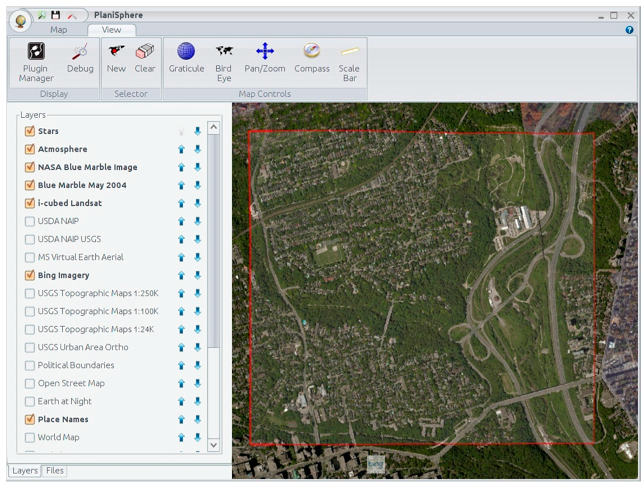
Figure 3.
PlaniSphere with the Plug-in Manager and Sample Plug-ins (JRE SysInfo and NMEA Parser).
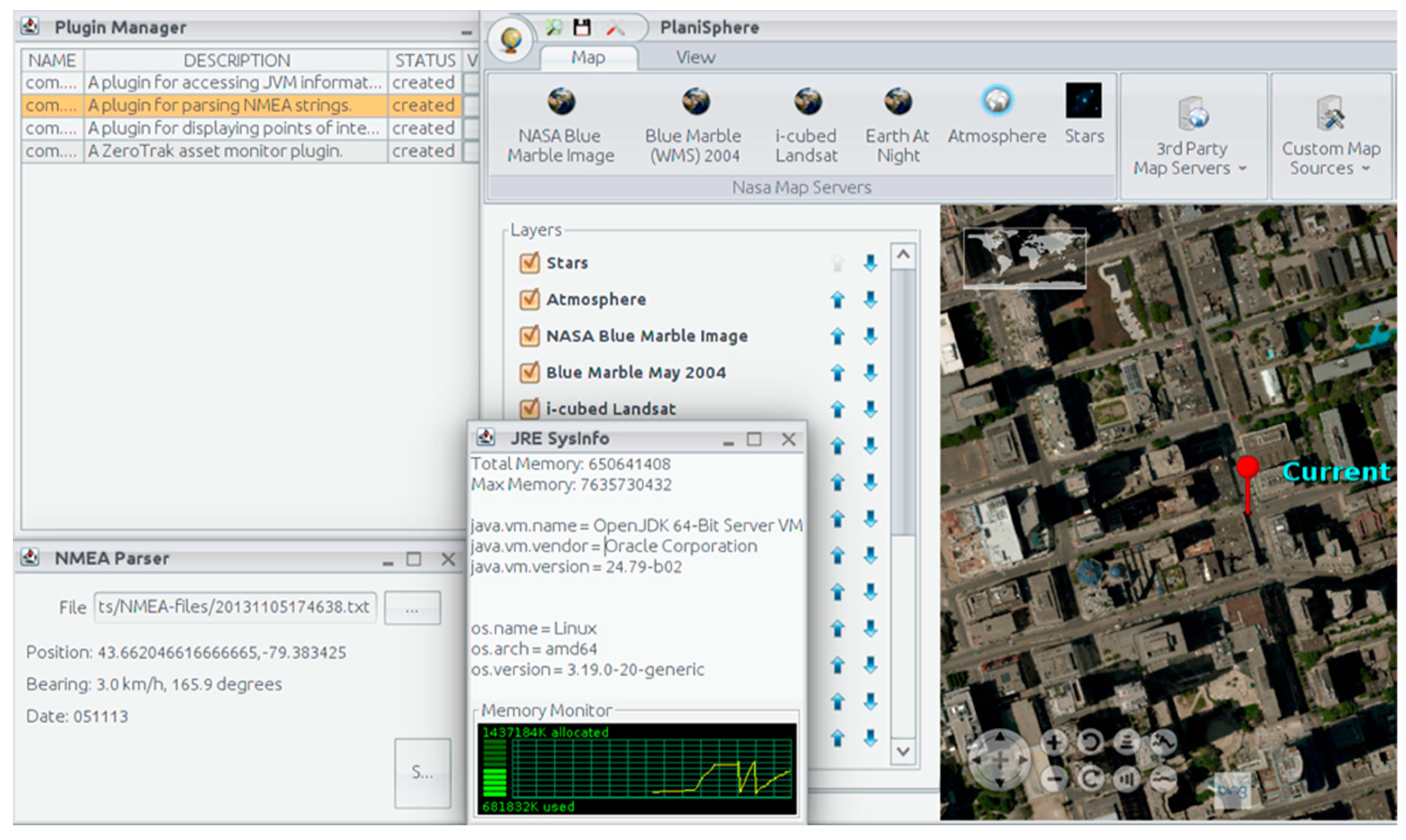
Figure 4.
Fusion of multiple layers from different WMS servers: (a) LandSat7 photograph of Toronto, (b) OpenStreetMap roadmap, (c) OpenStreetMap map superimposed over a LandSat photograph, and (d) After analyzing using Planisphere.
Figure 4.
Fusion of multiple layers from different WMS servers: (a) LandSat7 photograph of Toronto, (b) OpenStreetMap roadmap, (c) OpenStreetMap map superimposed over a LandSat photograph, and (d) After analyzing using Planisphere.

Figure 5.
A PlaniSphere plug-in demonstrating Online Analytical Processing (OLAP) capabilities by identifying areas of lower population concentration. Note the blue lines represent an extrapolated municipal border generated by analyzing population concentration on either side of the border.
Figure 5.
A PlaniSphere plug-in demonstrating Online Analytical Processing (OLAP) capabilities by identifying areas of lower population concentration. Note the blue lines represent an extrapolated municipal border generated by analyzing population concentration on either side of the border.

Figure 6.
Blue Marble Next Generation imagery and the Moon from the Jet Propulsion Laboratory WMS server: (a) Flat-Modified Sinusoidal Projection, (b) Mercator Projection, (c) Lunar Orbital Mosaic, Colorized and Shaded Elevation by a single layer, and (d) A detail view of several points of interest.

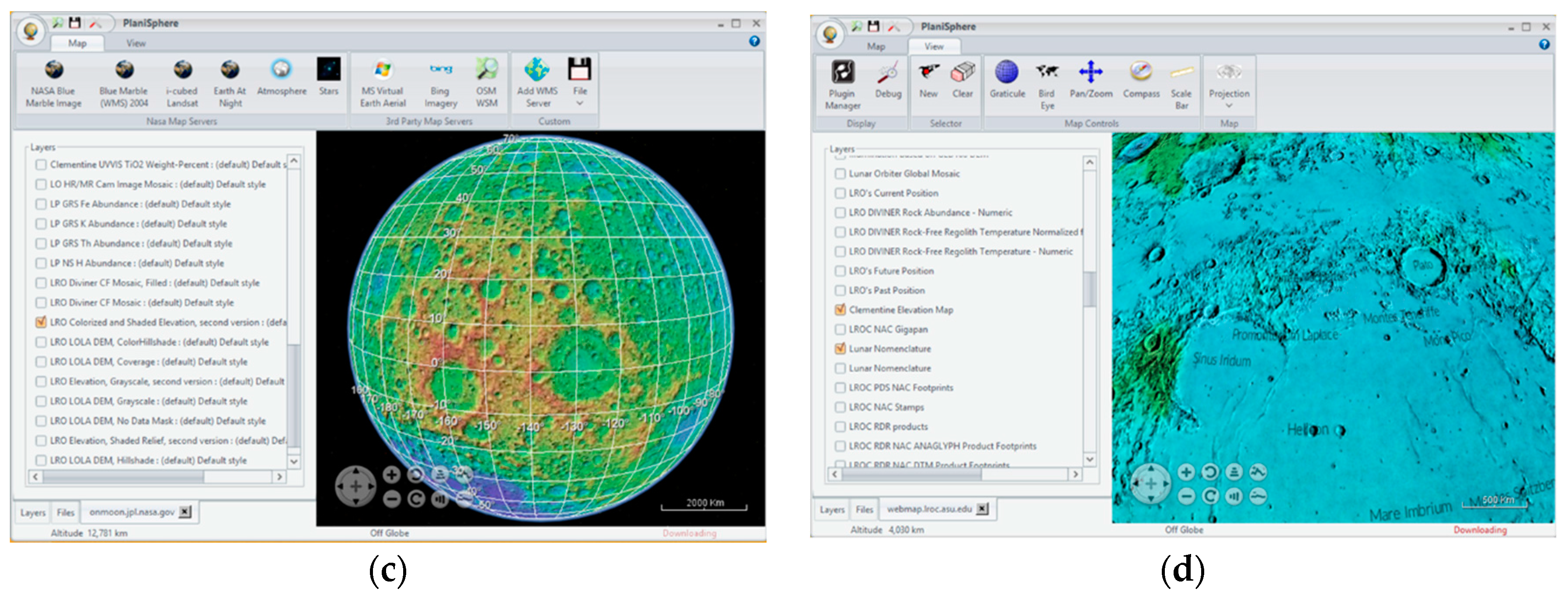
Figure 7.
A LiDAR cloud point map superimposed over a Bing aerial view of North Vancouver.
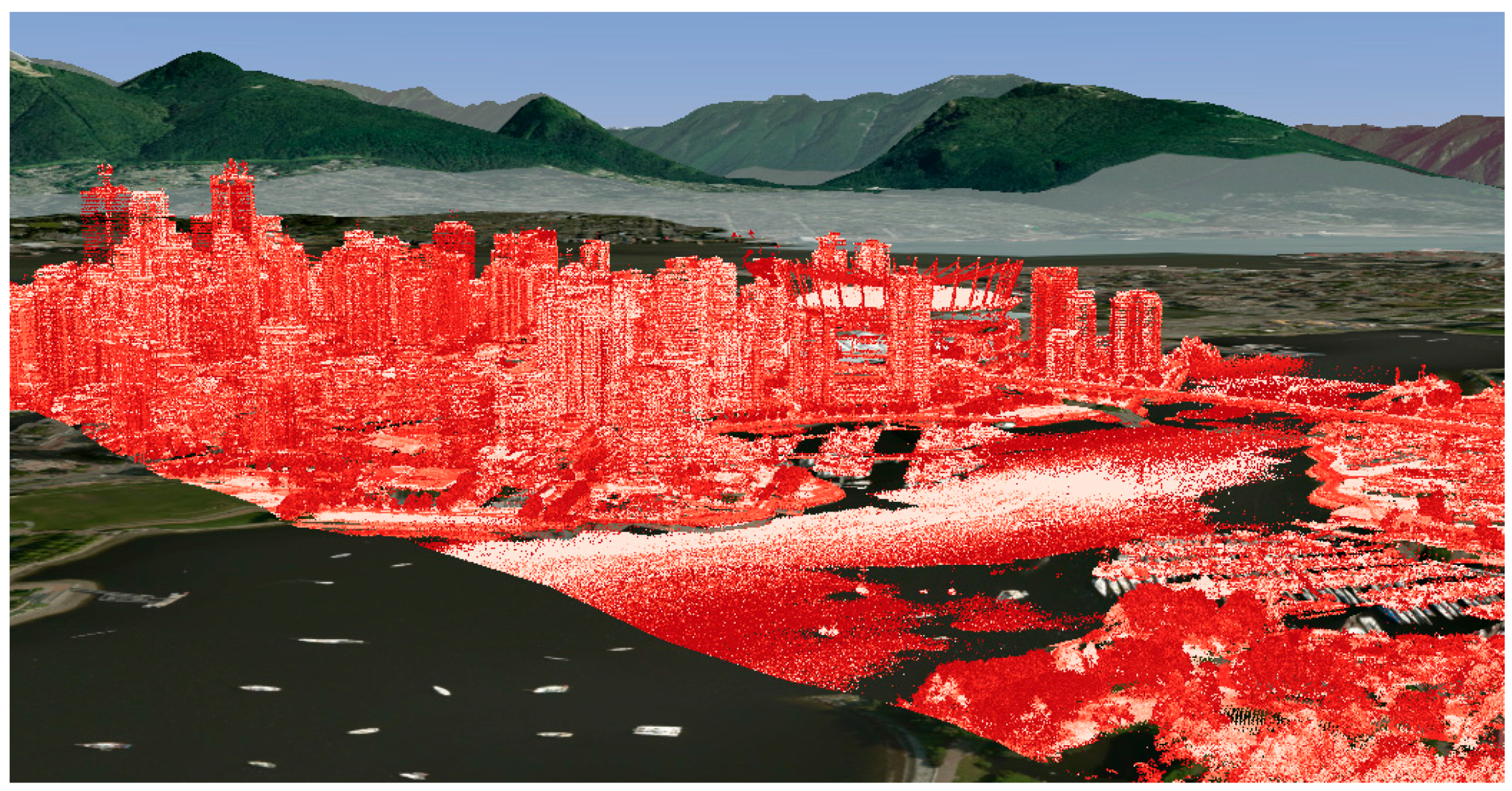
Figure 8.
A three-dimensional (3D) visualization with some hills and farm land superimposed over a Bing aerial two-dimensional (2D) map and data at an area near Cochrane, Alberta (51.1830, −114.4742).
Figure 8.
A three-dimensional (3D) visualization with some hills and farm land superimposed over a Bing aerial two-dimensional (2D) map and data at an area near Cochrane, Alberta (51.1830, −114.4742).

Table 1.
Files and Data Sources supported by PlaniSphere.
| Native Support (Out of Box Support by Planisphere) | 3rd Party Support | |
|---|---|---|
| Open Sources | Closed Sources | |
| Network/Internet | Local Files | Proprietary Files and Services |
| WMS | GeoJSON | SQL (may be supported by creating a plugin) |
| WFS (currently an experimental feature) | KML | Proprietary files (may be supported by creating a plugin) |
| Raster (TIFF, GeoTIFF) | Custom Web Services (may be supported by creating a plugin) | |
| ESRI Shape Files | ||
| LiDAR (LAS) | ||
© 2018 by the authors. Licensee MDPI, Basel, Switzerland. This article is an open access article distributed under the terms and conditions of the Creative Commons Attribution (CC BY) license (http://creativecommons.org/licenses/by/4.0/).
Share and Cite
MDPI and ACS Style
Miu, M.; Zhang, X.; Dewan, M.A.A.; Wang, J. Development of Framework for Aggregation and Visualization of Three-Dimensional (3D) Spatial Data. Big Data Cogn. Comput. 2018, 2, 9. https://doi.org/10.3390/bdcc2020009
AMA Style
Miu M, Zhang X, Dewan MAA, Wang J. Development of Framework for Aggregation and Visualization of Three-Dimensional (3D) Spatial Data. Big Data and Cognitive Computing. 2018; 2(2):9. https://doi.org/10.3390/bdcc2020009
Chicago/Turabian StyleMiu, Mihal, Xiaokun Zhang, M. Ali Akber Dewan, and Junye Wang. 2018. "Development of Framework for Aggregation and Visualization of Three-Dimensional (3D) Spatial Data" Big Data and Cognitive Computing 2, no. 2: 9. https://doi.org/10.3390/bdcc2020009