Function Modeling Improves the Efficiency of Spatial Modeling Using Big Data from Remote Sensing


Rocky Mountain Research Station, U.S. Forest Service, Missoula, MT 59801 USA
*
Author to whom correspondence should be addressed.
Big Data Cogn. Comput. 2017, 1(1), 3; https://doi.org/10.3390/bdcc1010003
Submission received: 26 June 2017
/
Revised: 10 July 2017
/
Accepted: 10 July 2017
/
Published: 13 July 2017
Abstract
:Spatial modeling is an integral component of most geographic information systems (GISs). However, conventional GIS modeling techniques can require substantial processing time and storage space and have limited statistical and machine learning functionality. To address these limitations, many have parallelized spatial models using multiple coding libraries and have applied those models in a multiprocessor environment. Few, however, have recognized the inefficiencies associated with the underlying spatial modeling framework used to implement such analyses. In this paper, we identify a common inefficiency in processing spatial models and demonstrate a novel approach to address it using lazy evaluation techniques. Furthermore, we introduce a new coding library that integrates Accord.NET and ALGLIB numeric libraries and uses lazy evaluation to facilitate a wide range of spatial, statistical, and machine learning procedures within a new GIS modeling framework called function modeling. Results from simulations show a 64.3% reduction in processing time and an 84.4% reduction in storage space attributable to function modeling. In an applied case study, this translated to a reduction in processing time from 2247 h to 488 h and a reduction is storage space from 152 terabytes to 913 gigabytes.
1. Introduction
Spatial modeling has become an integral component of geographic information systems (GISs) and remote sensing. Combined with classical statistical and machine learning algorithms, spatial modeling in GIS has been used to address wide ranging questions in a broad array of disciplines, from epidemiology [1] and climate science [2] to geosciences [3] and natural resources [4,5,6]. However, in most GISs, the current workflow used to integrate statistical and machine learning algorithms and to process raster models limits the types of analyses that can be performed. This process can be generally described as a series of sequential steps: (1) build a sample data set using a GIS; (2) import that sample data set into statistical software such as SAS [7], R [8], or MATLAB [9]; (3) define a relationship (e.g., predictive regression model) between response and explanatory variables that can be used within a GIS to create predictive surfaces, and then (4) build a representative spatial model within a GIS that uses the outputs from the predictive model to create spatially explicit surfaces. Often, the multi-software complexity of this practice warrants building tools that streamline and automate many aspects of the process, especially the export and import steps that bridge different software. However, a number of challenges place significant limitations on producing final outputs in this manner, including learning additional software, implementing predictive model outputs, managing large data sets, and handling the long processing time and large storage space requirements associated with this work flow [10,11]. These challenges have intensified over the past decade because large, fine-resolution remote sensing data sets, such as meter and sub-meter imagery and Lidar, have become widely available and less expensive to procure, but the tools to use such data efficiently and effectively have not always kept pace, especially in the desktop environment.
To address some of these limitations, advances in both GIS and statistical software have focused on integrating functionality through coding libraries that extend the capabilities of any software package. Common examples include RSGISlib [12], GDAL [13], SciPy [14], ALGLIB [15], and Accord.NET [16]. At the same time, new processing techniques have been developed to address common challenges with big data that aim to more fully leverage improvements in computer hardware and software configurations. For example, parallel processing libraries such as OpenCL [17] and CUDA [18] are stable and actively being used within the GIS community [19,20]. Similarly, frameworks such as Hadoop [21] are being used to facilitate cloud computing, and offer improvements in big data processing by partitioning processes across multiple CPUs within a large server farm, thereby improving user access, affordability, reliability, and data sharing [22,23]. While the integration, functionality, and capabilities of GIS and statistical software continue to expand, the underlying framework of how procedures and methods are used within spatial models in GIS tends to remain the same, which can impose artificial limitations on the type and scale of analyses that can be performed.
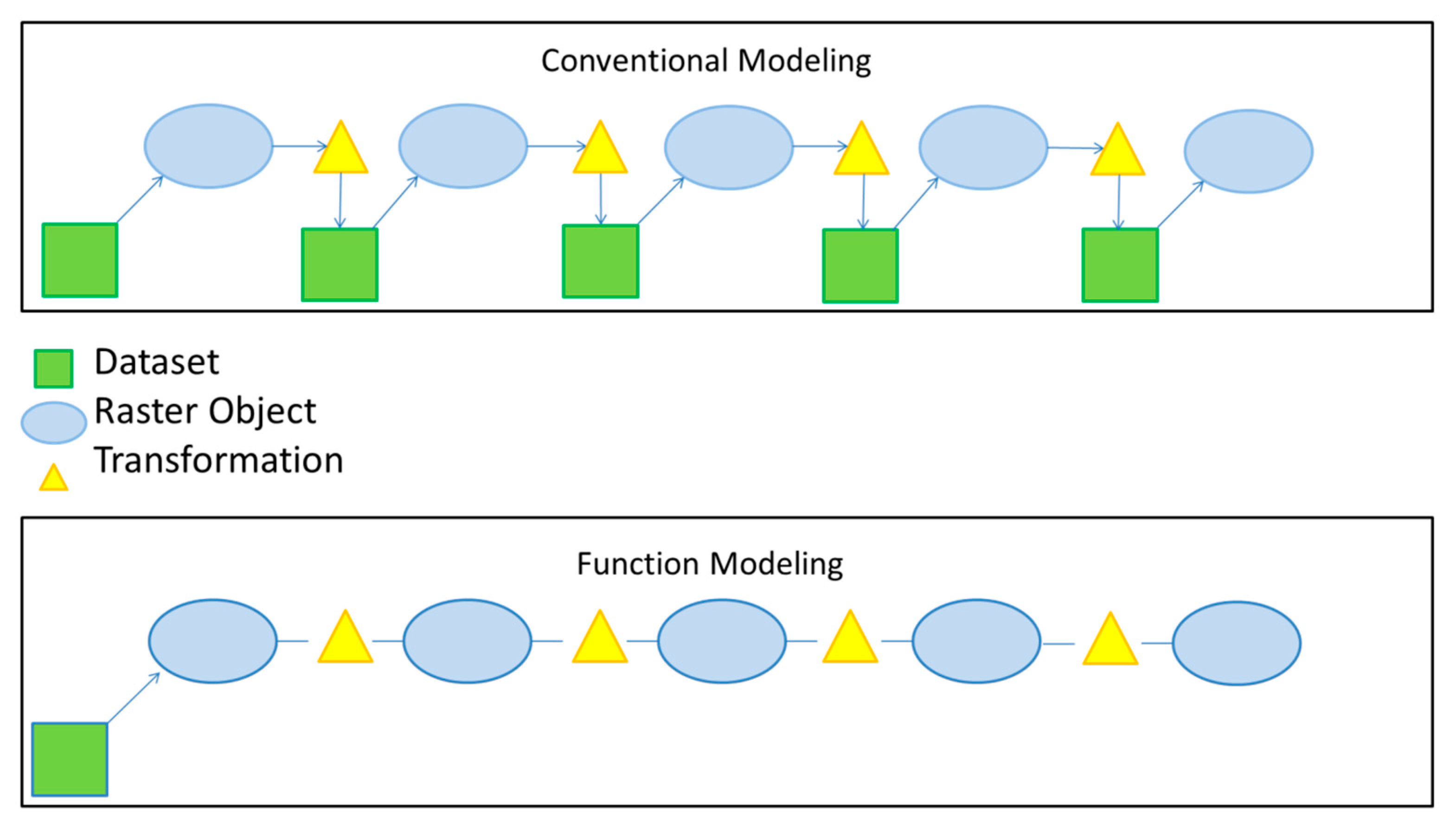
Spatial models are typically composed of multiple sequential operations. Each operation reads data from a given data set, transforms the data, and then creates a new data set (Figure 1). In programming, this is called eager evaluation (or strict semantics) and is characterized by a flow that evaluates all expressions (i.e., arguments) regardless of the need for the values of those expressions in generating final results [24]. Though eager evaluation is intuitive and used by many traditional programming languages, creating and reading new data sets at each step of a model in GIS comes at a high processing and storage cost, and is not viable for large area analysis outside of the supercomputing environment, which is not currently available to the vast majority of GIS users.
In contrast, lazy evaluation (also called lazy reading and call-by-need) can be employed to perform the same types of analyses, reducing the number of reads and writes to disk, which reduces processing time and storage. In lazy evaluation, actions are delayed until their results are required, and results can be generated without requiring the independent evaluation of each expression [24]. From a mathematical perspective, this is similar to function composition, in which functions are sequentially combined into a composite function that is capable of generating results without evaluating each function independently. The theoretical foundations of lazy evaluation employed in functional programming languages dates back to as early as 1971, as described by Jian et al. [25]. Tremblay [26], provides a thorough discussion of the different classes of functional programming languages and their expressiveness as it relates to the spectrum of strict and non-strict evaluation. He defines strict (i.e., eager) approaches as evaluating all of the arguments before starting the evaluation of the body of the function and evaluating the body of the function only if all arguments are defined, and lazy approaches as evaluating the body of the function before evaluating any of the arguments and evaluating the arguments only if needed while evaluating the body.
In GISs, operations in conventional spatial models are evaluated and combined eagerly in ways that generate intermediate data sets whose values are written to disk and used to produce final results. In a lazy evaluation context, evaluation is delayed, intermediate datasets are only generated if needed, and final data sets are not stored to disk but are instead processed dynamically when needed (Figure 1). For example, though an analysis may be conducted over a very large area at high resolution, final results can be generated easily in a call-by-need fashion for a smaller extent being visualized on a screen or map, without generating the entire data set for the full extent of the analysis.
In this paper, we introduce a new GIS spatial modeling framework called function modeling (FM) and highlight some of the advantages of processing big data spatial models using lazy evaluation techniques. Simulations and two case studies are used to evaluate the costs and benefits of alternative methods, and an open source .Net coding library built around ESRI (Redlands, CA, USA) ArcObjects is discussed. The coding library facilitates a wide range of big data spatial, statistical, and machine learning type analyses, including FM.
2. Materials and Methods
2.1. NET Libraries
To streamline the spatial modeling process, we developed a series of coding libraries that leverage concepts of lazy evaluation using function raster data sets [10,11] and integrate numeric, statistical, and machine learning algorithms with ESRI’s ArcObjects [27]. Combined, these libraries facilitate FM, which allows users to chain modeling steps and complex algorithms into one raster data set or field calculation without writing the outputs of intermediate modeling steps to disk. Our libraries were built using an object-oriented design, .NET framework, ESRI’s ArcObjects [27], ALGLIB [15], and Accord.net [16], which are accessible to computer programmers and analysts through our subversion site [28] and packaged in an add-in toolbar for ESRI ArcGIS [11]. The library and toolbar together are referred to here as the U.S. Forest Service Rocky Mountain Research Station Raster Utility (the RMRS Raster Utility) [28].
The methods and procedures within the RMRS Raster Utility library parallel many of the functions found in ESRI’s Spatial Analyst extension including focal, aggregation, resampling, convolution, remap, local, arithmetic, mathematical, logical, zonal, surface, and conditional operations. However, the libraries used in this study support multiband manipulations and perform these transformations without writing intermediate or final output raster data sets to disk. The spatial modeling framework used in the Utility focuses on storing only the manipulations occurring to data sets and applying those transformations dynamically at the time data are read. In addition to including common types of raster transformations, the utility also includes multiband manipulation procedures such as gray level co-occurrence matrix (GLCM), time series transformations, landscape metrics, entropy and angular second moment calculations for focal and zonal procedures, image normalization, and other statistical and machine learning transformations that are integrated directly into this modeling framework.
While the statistical and machine learning transformations can be used to build surfaces and calculate records within a tabular field, they do not in themselves define the relationships between response and explanatory variables like a predictive model. To define these relationships, we built a suite of classes that perform a wide variety of statistical testing and predictive modeling using many of the optimization algorithms and mathematical procedures found within ALGLIB and Accord.net [15,16]. Typically, in natural resource applications that use GIS, including the case studies presented in Section 2.3, analysts use samples drawn from a population to test hypotheses and create generalized associations (e.g., an equation or procedure) between variables of interest that are expensive to collect in the field (i.e., response variables) and variables that are less costly and thought to be related to the response variables (i.e., explanatory variables; Figure 2 and Figure 3). For example, it is common to use the information contained in remotely sensed images to predict the physical characteristics of vegetation that is otherwise measured accurately and relatively expensively with ground plots. While the inner workings and assumptions of the algorithms used to develop these relationships are beyond the scope of this paper, it is worth noting that the classes developed to utilize these algorithms within a spatial context provide computer programmers and analysts with the ability to use these techniques in the FM context, relatively easily without developing code for such algorithms themselves.
Combined with FM, the sampling, modeling, and surface creation workflow can be streamlined to produce outputs that answer questions and display relationships between response and explanatory variables in a spatially explicit manner. However, improvements in efficiency and effectiveness over conventional techniques are not always known. These .NET libraries were used to test the hypothesis that FM provides significant improvement over conventional techniques and to quantify any related effects on storage and processing time.
2.2. Simulations
From a theoretical standpoint, FM should improve processing efficiency by reducing the processing time and storage space associated with spatial modeling, primarily because it requires fewer input and output processes. However, to justify the use of FM methods, it is necessary to quantify the extent to which FM actually reduces processing time and storage space. To evaluate FM, we designed, ran, and recorded processing time and storage space associated with six simulations, each including 12 models, varying the size of the raster data sets used in each simulation. From the results of those simulations, we compared and contrasted FM with conventional modeling (CM) techniques using linear regression and analysis of covariance (ANCOVA). All CM techniques were directly coded against ESRI’s ArcObject Spatial Analyst classes to minimize CM processing time and provide a fair comparison.
Spatial modeling scenarios within each simulation ranged from one arithmetic operation to twelve operations that included arithmetic, logical, conditional, focal, and local type analyses. Counts of each type of operation included in each model are shown in Table 1. In the interest of conserving space, composite functions for each of these models are not included and defined here, but, as described in the introduction, each model could be presented in mathematical form. Each modeling scenario created a final raster output and was run against six raster data sets ranging in size from 1,000,000 to 121,000,000 total cells (1 m2 grain size), incrementally increasing in total raster size by 2000 columns and 2000 rows at each step (adding 4 million cells at each step, Figure 4). Cell bit depth remained constant as floating type numbers across all scenarios and simulations. Simulations were carried out on a Hewlett-Packard EliteBook 8740 using an I7 Intel quad core processor and standard internal 5500 revolutions per minute (RPM) hard disk drives (HHD).
These simulations employed stepwise increases in the total number of cells used in the analysis. It is worth noting here that this is a different approach than maintaining a fixed area (i.e., extent) and changing granularity, gradually moving from coarse to fine resolution and larger numbers of smaller and smaller cells. In this simulation, the algorithm used would produce the same result in both situations. However, some algorithms identify particular structures in an image and try to use characteristics like structural patterns and local homogeneity to improve efficiency, especially when attempting to discern topological relations, potentially using map-based measurements in making such determinations. In these cases, granularity may be important, and comparing the performance of different approaches would benefit from using both raster size and grain size simulations.
To determine the overhead of creating and using a FM, we also conducted a simulation using focal mean analyses that varied neighborhood window size across six images. Each iteration of the simulation gradually increased the neighborhood window size for the focal mean procedure from a 10 by 10 to a 50 by 50 cell neighborhood (in increments of 10 cells) to evaluate the impact of processing more cells within a neighborhood, while holding the image and number of input and output procedures constant. Images used in this simulation were the same as in the previous simulation and contained between 1,000,000 and 121,000,000 total cells. In this scenario, CM and FM techniques were expected to show no difference with regard to processing time and storage space using a paired t-test comparison, and any differences recorded in processing or storage can be attributed to the overhead associated with creating and using a FM.
2.3. Case Studies
To more fully explore the use of FM to analyze data and create predictive surfaces in real applications, we evaluated the efficiencies associated with two case studies: (1) a recent study of the Uncompahgre National Forest (UNF) in the US state of Colorado [6,29] and (2) a study focused on the forests of the Montana State Department of Natural Resources and Conservation (DNRC) [unpublished data]. For the UNF study, we used FM, fixed radius cluster plots, and fine resolution imagery to develop a two-stage classification and estimation procedure that predicts mean values of forest characteristics across 1 million ha at a spatial resolution of 1 m2. The base data used to create these predictions consisted of National Agricultural Imagery Program (NAIP) color infrared (CIR) imagery [30], which contained a total of 10 billion pixels for the extent of the study area. Within this project, we created no fewer than 365 explanatory raster surfaces, many of which represented a combination of multiple raster functions, as well as 52 predictive models, and 64 predictive surfaces. All of these outputs were generated at the extent and spatial resolution of the NAIP imagery (1 m2, 10 billion pixels).
For the DNRC study, we used FM, variable radius plots, and NAIP imagery to predict basal area per acre (BAA), trees per acre (TPA), and board foot volume per acre (BFA) for more than 2.2 billion pixels (~0.22 million ha) in northwest Montana USA at the spatial resolution of 1 m2. In this study, we created 12 explanatory variables, three predictive models, and three raster surfaces depicting mean plot estimates of BAA, TPA, and BFA. Average plot extent was used to extract spectral and textural values in the DNRC study and was determined by calculating average limiting distance of trees within each plot given the basal area factor used in the field measurement (ranging between 5 and 20) and the diameter of each tree measured.
While it would be ideal to directly compare CM with FM for the UNF and DNRC case studies, ESRI’s libraries do not have procedures to perform many of the analyses and raster transformations used in these studies, so CM was not incorporated directly into the analysis. As an alternative to evaluate the time savings associated with using FM in these examples, we used our simulated results and estimated the number of individual CM functions required to create GLCM explanatory variables and model outputs. Processing time was based on the number of CM functions required to produce equivalent explanatory variables and predictive surfaces. In many instances, multiple CM functions were required to create one explanatory variable or final output. The number of functions were then multiplied by the corresponding proportion increase in processing time associated with CM when compared to FM. Storage space was calculated based on the number of intermediate steps used to create explanatory variables and final outputs. In all cases, the space associated with intermediate outputs from FM and CM were calculated without data compression and summed to produce a final storage space estimate.
3. Results
3.1. Simulations
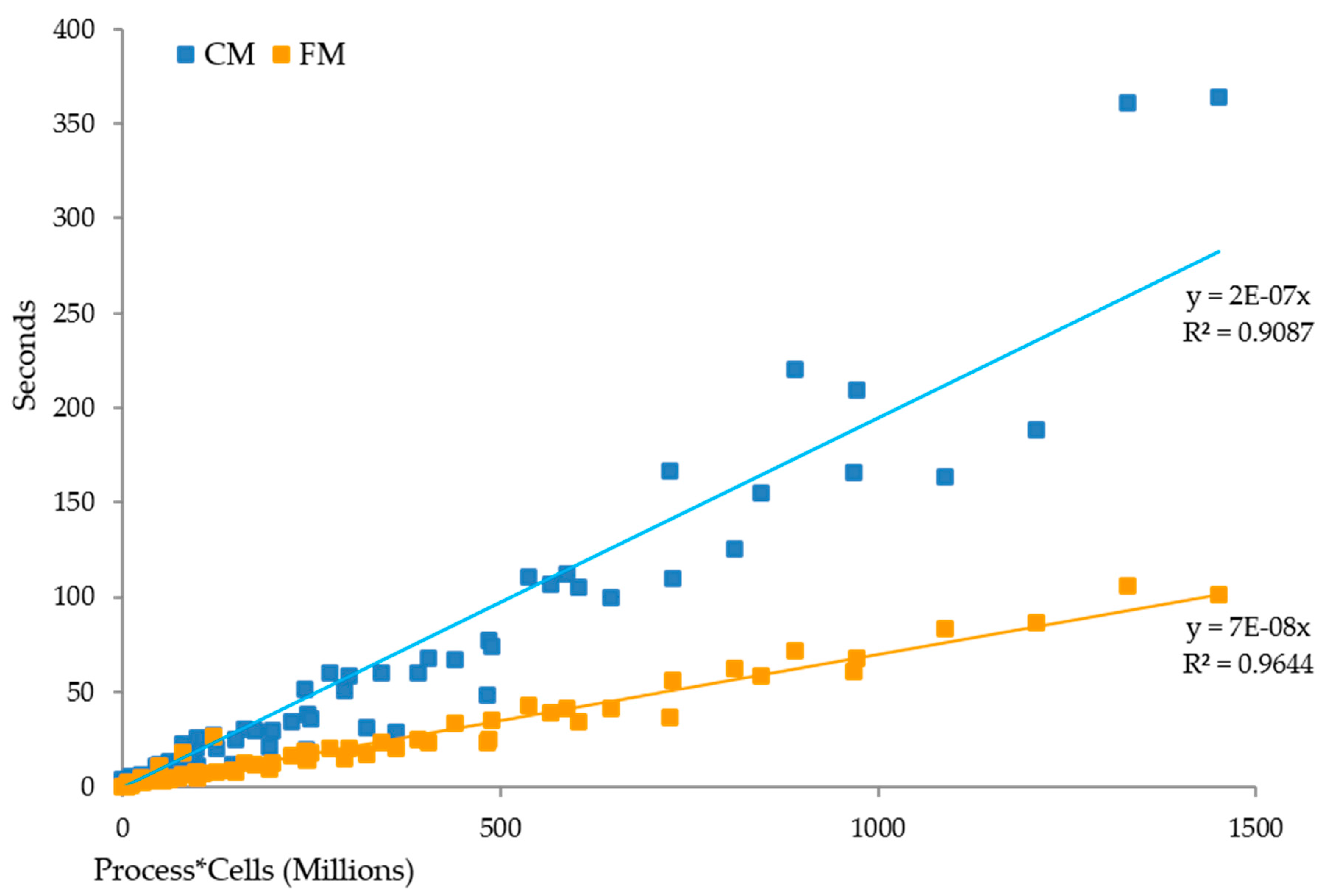
To evaluate the gains in efficiency of FM, we compared it with CM across six simulations, each running 12 models of increasing complexity. FM significantly reduced both processing time (Fdf,1 = 303.89; p-value < 0.001) and storage space (Fdf,1 = 3.64; p-value = 0.058) when compared to CM (Figure 5 and Figure 6). FM took 26.13 m and a total of 13,299.09 megabytes to perform all six simulations, while CM took 73.15 m and 85,098.27 megabytes. This represents a 2.8-fold increase in processing time and a 6.4-fold increase in storage space moving from FM to CM. Theoretically, processing time and storage space associated with creating raster data for a given model, computer configuration, set of operations, and data type should be a linear function of the total number of cells within a raster data set and the total number of operations within the model, as shown by:
where i denotes the technique, either FM or CM in this case. Our empirically derived FM time and space models nicely fit the linear paradigm (R2 = 0.96 and 0.99, respectively). However, for the CM techniques, the model for Time (R2 = 0.91) deviated slightly and the model for Space (R2 = 0.10) deviated substantially from theoretical distributions, indicating that, in addition to the modeling operations, extra operations occurred to facilitate raster processing and that some of those extra operations produced intermediate raster data sets, generating wider variation in time and space requirements than would be expected based on these equations (Equation (1)).
Timei (seconds) = βi(cells × operations)i
Spacei (megabytes) = βi (cells)i
Spacei (megabytes) = βi (cells)i
CM and FM time equation coefficients indicate that, on average, CM processing time was 278% longer than FM processing time—a nearly three-fold increase in proceeding time. Model fit for FM and CM space equations varied greatly between techniques and could not be compared reliably in the same manner. For the CM methodology, storage space appeared to vary depending on the types of operations within the model and often decreased well after the creation of the final data set. This outcome is assumed to be caused by delayed removal of intermediate data sets. Overall though, CM total storage space was 640% larger than FM storage space for the six simulations.
When comparing processing time and storage space between FM and CM techniques for varying neighborhood window sizes, there was a substantial difference between the two methods (Figure 7; paired t-testdf,29 = 3.82; p-value < 0.001). As expected, processing time increased as the number of cells increased within the neighborhood window, while storage space remained the same across CM and FM iterations. However, FM processing time was significantly faster than CM processing time and CM storage space was twice that of FM. Upon further inspection, these differences stem from the creation of intermediate data sets for the CM procedure even when only one process is specified and also from differences in the underlying algorithms for calculating mean values within a focal neighborhood window.
3.2. UNF and DNRC Case Studies
Although simulated results quantify improvements related to using FM, the UNF and DNRC case studies illustrate these efficiencies in a more concrete and applied manner. In the UNF study, we created no fewer than 365 explanatory raster surfaces, 52 predictive models, and 64 predictive surfaces at the extent and spatial resolution of the NAIP imagery (1 million ha study area at 1 m2 resolution). To compare the two approaches, it was assumed that all potential explanatory surfaces were created for CM to facilitate sampling and statistical model building. In contrast, FM only sampled explanatory surfaces and calculated values for the variables selected in the final models.
As described previously, CM was not incorporated directly into the analysis because ESRI’s libraries do not have procedures to perform many of the analyses and raster transformations required. CM performance was estimated based on the results of simulations. For the land cover classification stage of the UNF study, we estimated that to reproduce the explanatory variables and probabilistic outputs using CM techniques, it would take approximately 283 processing h on a Hewlett-Packard EliteBook 8740 using an I7 Intel quad core processor and internal 5500 RPM HHD and would require at least 19 terabytes of storage space. Using FM, these same procedures took approximately 37 processing h and a total of 140 gigabytes of storage space. Similarly, for the second stage of the classification and estimation approach, we estimated a processing time of approximately 2247 h with an associated storage requirement of 152 terabytes using CM. Using FM, these same procedures took approximately 488 h and required roughly 913 gigabytes of storage.
For the DNRC case study, we estimated that to create the explanatory and final predictive surfaces using CM would require building 30 raster surfaces taking approximately 97 h to complete and 239.3 gigabytes of storage space. Using FM, this same procedure took approximately 21 h to complete and only 24.7 gigabytes of storage space (Figure 8).
4. Discussion
The underlying concept behind FM is lazy evaluation, which has been used in programming for decades, and is conceptually similar to function composition in mathematics. Using this technique in GIS removes the need to store intermediate data sets to disk in the spatial modeling process and allows models to process data only for the spatial areas needed at the time they are read. In CM, as spatial models become more complex (i.e., more modeling steps) the number of intermediate outputs increases. These intermediate outputs significantly increase the amount of processing time and storage space required to run a specified model. In contrast, FM does not store intermediate data sets, thereby significantly reducing model processing time and storage space.
In this study, we quantified this effect by comparing FM to CM methodologies using simulations that created final raster outputs from multiple, incrementally complex models. However, this does not capture the full benefit of operating in the FM environment. Because FM does not need to store outputs to disk in a conventional format (e.g., Grid or Imagine format), and all functions occurring to source raster data sets can be stored and used in a dynamic fashion to display, visualize, symbolize, retrieve, and manipulate function data sets at a small fraction of the time and space it takes to create a final raster output, this framework allows extremely efficient work flows and data exploration. For example, if we were to perform the same six simulations presented here but replace the requirement of storing the final output as a conventional raster format with creating a function model, it would take less than 1 second and would require less than 50 kilobytes of storage to finish the same simulations. The results can then be stored as a conventional raster at a later time if needed. To further illustrate this point, we conducted a simulation to quantify the time and storage required to create various size data sets from a function in FM, and then read it back into a raster object using various neighborhood window sizes. Results show that storage space and processing time to read FM objects are extremely small (kilobytes and milliseconds) and that the underlying algorithms behind those procedures have a much larger impact than the overhead associated with lazy evaluation. Based on these results, for the UNF and DNRC case studies, FM facilitated an analysis that simply would have been too lengthy (and costly) to perform using CM.
Though it is gaining traction, the majority of GIS professionals use CM and have not been exposed to FM concepts. Furthermore, FM is not included in most “off-the-shelf” GISs, making it difficult for the typical analyst to make the transition, even if FM results in better functionality, significant efficiency gains, and improved work flow. Also, even if coding libraries are available, many GIS users do not have the programming skills necessary to execute FM outside of a graphical interface of some kind. To simplify and facilitate the use of FM and complex statistical and machine learning algorithms within GIS, we have created a user-friendly add-in toolbar called the RMRS Raster Utility (Figure 9) that provides quick access to a wide array of spatial analyses, while allowing users to easily store and retrieve FM models. The toolbar was specifically developed for ESRI’s GIS, one of the most widely used commercial platforms, but the underlying libraries have applicability in almost all GISs. Using the toolbar in the ESRI environment, FM models can be loaded into ArcMap as a function raster data set and can be used interchangeably with all ESRI raster spatial operations.
Currently, our solution contains 1016 files, over 105,000 lines of code, 609 classes, and 107 forms that facilitate functionality ranging from data acquisition to raster manipulation, and statistical and machine learning types of analyses, in addition to FM. Structurally, the utility contains two primary projects that consist of an ESRI Desktop class library (“esriUtil”) and an ArcMap add-in (“servicesToolBar”). The project esriUtil contains most of the functionality of our solution, while the servicesToolBar project wraps that functionality into a toolbar accessible within ArcMap. In addition, two open source numeric class libraries are used within our esriUtil project. These libraries, ALGLIB [15] and Accord.net [16], provide access to numeric, statistical, and machine learning algorithms used to facilitate the statistical and machine learning procedures within our classes.
While FM is efficient compared to CM and uses almost no storage space, there may be circumstances that warrant saving FMs to disk in a conventional raster format. Obviously, if intermediate data sets are useful products in themselves or serve as necessary inputs for other, independent FMs, FMs can be saved as conventional raster data sets at any point along the FM chain. For example, if one FM (FM1) is read multiple times to create a new FM (FM2) and the associated time it takes to read multiple instances of FM1 is greater than the combined read and write time of saving FM1 to a conventional raster format (i.e., many transformations within the first FM), then it would be advantageous to save FM1 to a conventional raster format and use the newly created conventional raster data set in FM2. Also, some processes that are hierarchical in nature where the same operations occur for multiple embedded processes may benefit from a similar strategic approach to storing specific steps in a FM as a conventional raster data set. Nonetheless, results from our simulations and case studies demonstrate that FM substantially reduces processing time and storage space. Given accessible tools and appropriate training, GIS professionals may find that these benefits outweigh the costs of learning new techniques to incorporate FM into their analysis and modeling of large spatial data sets.
Acknowledgments
This work was funded by the United States Department of Agriculture (USDA), US Forest Service, Rocky Mountain Research Station, and by the USDA National Institute of Food and Agriculture, Biomass Research and Development Initiative award no. 2011-10006-30357 and Agriculture and Food Research Initiative Competitive award no. 2013-68005-21298.
Author Contributions
John Hogland proposed, built, and applied the concepts of Function Modeling, developed the RMRS Raster Utility coding libraries and repository, designed and implemented the simulations and case studies, and contributed to the writing of the manuscript; Nathaniel Anderson contributed to the writing of the manuscript and the development of figures and tables, described the theoretical background of eager and lazy evaluation coding strategies, and contributed to the design of the simulations and case studies.
Conflicts of Interest
The authors declare no conflict of interest.
References
- Auchincloss, A.H.; Gebreab, S.Y.; Mair, C.; Diez Roux, A.V. A Review of Spatial Methods in Epidemiology, 2000–2010. Annu. Rev. Public Health 2012, 33, 107–122. [Google Scholar] [CrossRef] [PubMed]
- Patenaude, G.; Milne, R.; Dawson, T. Synthesis of remote sensing approaches for forest carbon estimation Reporting to the Kyoto Protocol. Environ. Sci. Policy 2005, 8, 161–178. [Google Scholar] [CrossRef]
- Pradhan, B.; Lee, S.; Buchroithner, M.F. A GIS-based back-propagation neural network model and its cross-application and validation for landslide susceptibility analyses. Comput. Environ. Urban Syst. 2010, 34, 216–235. [Google Scholar] [CrossRef]
- Martin, P.H.; LeBoeuf, E.J.; Dobbins, J.P.; Daniel, E.B.; Abkowitz, M.D. Interfacing GIS with water resource models: A state-of-the-art. J. Am. Water Resour. Assoc. 2005, 41, 1471–1487. [Google Scholar] [CrossRef]
- Reynolds-Hogland, M.; Mitchell, M.; Powell, R. Spatio-temporal availability of soft mast in clearcuts in the Southern Appalachians. For. Ecol. Manag. 2006, 237, 103–114. [Google Scholar]
- Wells, L.A.; Chung, W.; Anderson, N.M.; Hogland, J.S. Spatial and temporal quantification of forest residue volumes and delivered costs. Can. J. For. Res. 2016, 46, 832–843. [Google Scholar] [CrossRef]
- SAS Institute. SAS/STAT(R) 9.3 User’s Guide. Available online: https://support.sas.com/documentation/cdl/en/statug/63962/HTML/default/viewer.htm#titlepage.htm (accessed on 3 March 2017).
- The R Project for Statistical Computing. Available online: http://www.r-project.org/ (accessed on 3 March 2017).
- MATLAB. MathWorks-MATLAB and Simulink for Technical Computing. Available online: http://www.mathworks.com/ (accessed on 3 March 2017).
- Hogland, J.S.; Anderson, N.M. Improved analyses using function datasets and statistical modeling. In Proceedings of the 2014 ESRI Users Conference, San Diego, CA, USA, 14–18 July 2014; Environmental Systems Research Institute: Redlands, CA, USA, 2014; pp. 1–14. [Google Scholar]
- Hogland, J.S.; Anderson, N.M. Estimating FIA Plot Characteristics Using NAIP Imagery, Function Modeling, and the RMRS Raster Utility Coding Library; U.S. Department of Agriculture, Forest Service, Pacific Northwest Research Station: Portland, OR, USA, 2015; pp. 340–344. [Google Scholar]
- Bunting, P.; Clewley, D.; Lucas, R.M.; Gillingham, S. The Remote Sensing and GIS Software Library (RSGISLib). Comput. Geosci. 2014, 62, 216–226. [Google Scholar] [CrossRef]
- GDAL. GDAL—Geospatial Data Abstraction Library: Version 2.2.1, 2017, Open Source Geospatial Foundation. Available online: http://gdal.osgeo.org (accessed on 11 July 2017).
- Jones, E.; Oliphant, E.; Peterson, P. SciPy: Open Source Scientific Tools for Python, 2001. Available online: http://www.scipy.org/ (accessed on 11 July 2017).
- Bochkanov, S. ALGLIB. Available online: http://www.alglib.net/ (accessed on 3 March 2017).
- Souza, C. Accord.Net Framework. Available online: http://accord-framework.net/ (accessed on 3 March 2017).
- Banger, R.; Bhattacharyya, K. OpenCL Programming by Example; Packt Pyblishing Ltd.: Birmingham, UK, 2013; p. 304. [Google Scholar]
- Sanders, J.; Kandrot, E. CUDA by Example: and Introduction to General-Purpose GPU Programming; Addison-Wesley: Upper Saddle River, NJ, USA, 2011; p. 290. [Google Scholar]
- Ortega, L.; Rueda, A. Parallel drainage network computation on CUDA. Comput. Geosci. 2010, 36, 171–178. [Google Scholar] [CrossRef]
- Walsh, S.; Saar, M.; Baily, M.; Lilja, D. Accelerating geoscience and engineering system simulations on graphics hardware. Comput. Geosci. 2009, 35, 2353–2364. [Google Scholar] [CrossRef]
- White, T. Hadoop the Definitive guide, 4th Edition Storage and Analysis at Internet Scale; O’Reilly Media: Sebastopol, CA, USA, 2012; p. 756. [Google Scholar]
- Yang, C.; Michael, G.; Huang, Q.; Nebert, D.; Raskin, R.; Xu, Y.; Bambacus, M.; Fay, D. Spatial cloud computing: How can the geospatial sciences use and help shape cloud computing? Int. J. Digit. Earth 2011, 4, 305–329. [Google Scholar] [CrossRef]
- Xia, J.; Yang, C.; Liu, K.; Gui, Z.; Li, Z.; Huang, Q.; Li, R. Adopting cloud computing to optimize spatial web portals for better performance to support Digital Earth and other global geospatial initiatives. Int. J. Digit. Earth 2015, 8, 451–475. [Google Scholar] [CrossRef]
- Launchbury, J. Lazy imperative programming. In Proceedings of the ACM Sigplan Workshop on State in Programming Languages, Copenhagen, Denmark, June 1993; Yale University Research Report YALEU/DCS/RR-968. Yale University: New Haven, CT, USA; pp. 46–56. [Google Scholar]
- Jian, S.; Liu, K.; Wang, X. A survey on concepts and state of the art of functional programming languages. Systems and Computer Technology. In Proceedings of the 2014 International Symposium on Systems and Computer Technology, Shanghai, China, 15–17 November 2014; Taylor and Francis Group: London, UK, 2014; pp. 71–77. [Google Scholar]
- Tremblay, G. Lenient evaluation is neither strict nor lazy. Comput. Lang. 2000, 26, 43–66. [Google Scholar] [CrossRef]
- ESRI. ArcObjects SDK 10 Microsoft .Net Framework—ArcObjects Library Reference (Spatial Analyst). Available online: http://help.arcgis.com/en/sdk/10.0/arcobjects_net/componenthelp/index.html#/PrincipalComponents_Method/00400000010q000000/ (accessed on 3 March 2017).
- U.S. Forest Service Software Center. RMRS Raster Utility. Available online: https://collab.firelab.org/software/projects/rmrsraster (accessed on 3 March 2017).
- Hogland, J.; Anderson, N.; Chung, W.; Wells, L. Estimating forest characteristics using NAIP imagery and ArcObjects. In Proceedings of the 2014 ESRI Users Conference, San Diego, CA, USA, 14–18 July 2014; Environmental Systems Research Institute: Redlands, CA, USA, 2014; pp. 1–22. [Google Scholar]
- U.S. Department of Agriculture. National Agriculture Imagery Program (NAIP) Information Sheet. Available online: http://www.fsa.usda.gov/Internet/FSA_File/naip_info_sheet_2013.pdf (accessed on 3 March 2017).
Figure 1.
A schematic comparing conventional modeling (CM), which employs eager evaluation, to function modeling (FM), which uses lazy evaluation. The conceptual difference between the two modeling techniques is that FM delays evaluation until results are needed and produces results without storing intermediate data sets to disk (green squares). When input and output operations or disk storage space are the primary bottlenecks in running a spatial model, this difference in evaluation can substantially reduce processing time and storage requirements.

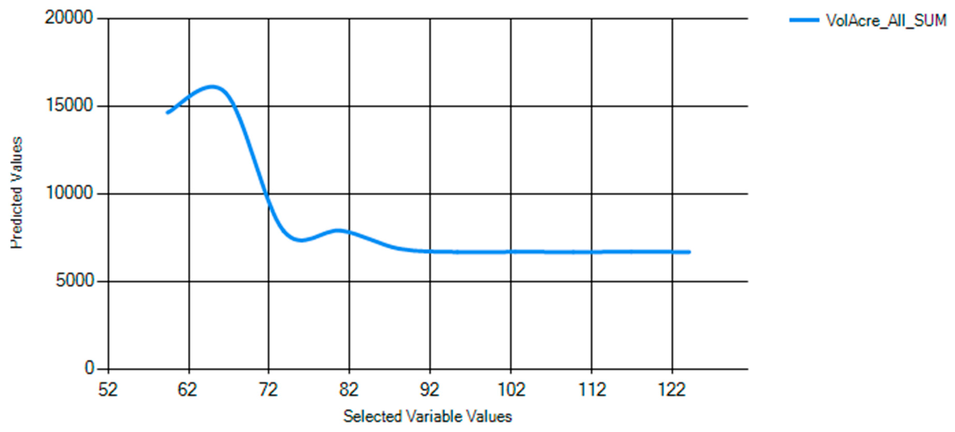
Figure 2.
An example of the types of interactive graphics produced within the RMRS Raster Utility toolbar that visually describe the generalized association (predictive model) between board foot volume per acre of trees greater than 5 inches in diameter (the response variable) and twelve explanatory variables derived from remotely sensed imagery. The figure illustrates the functional relationship between volume and one explanatory variable called “mean-Band3”, while holding all other explanatory variables values at 30% of their sampled range.

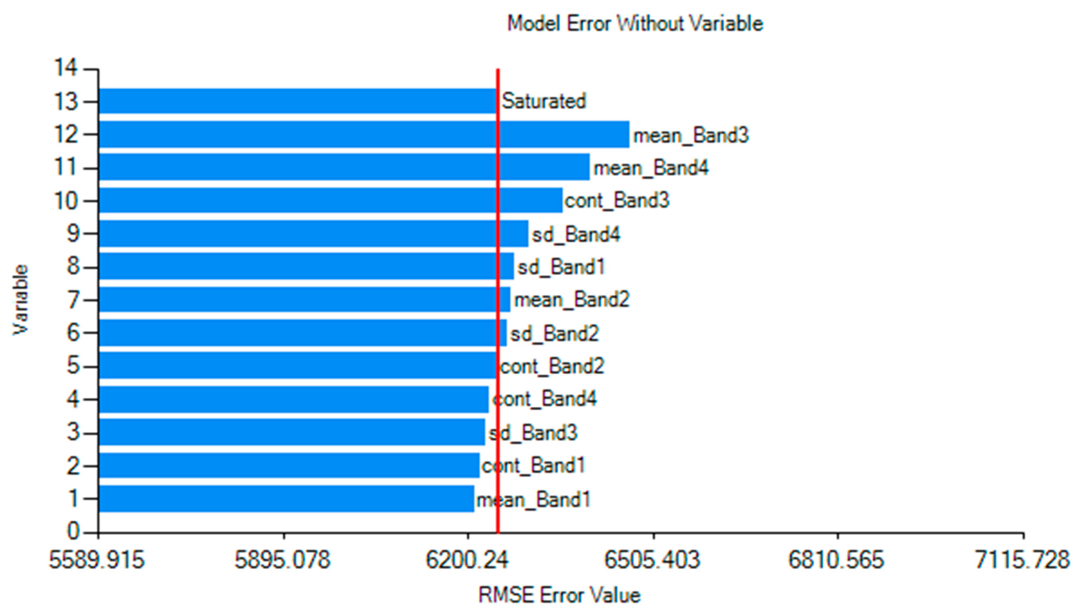
Figure 3.
An example of the interactive graphics produced within the RMRS Raster Utility toolbar that depicts the importance of each variable within a predictive model by systematically removing one variable from the model and comparing changes in root mean squared error (RMSE). The model used is a generalized association between board foot volume per acre and twelve explanatory variables derived from remotely sensed imagery, and was developed using a random forest algorithm and the RMRS Raster Utility toolbar.

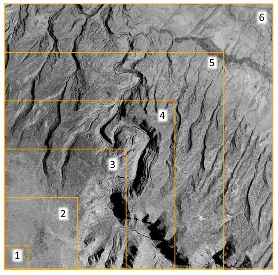
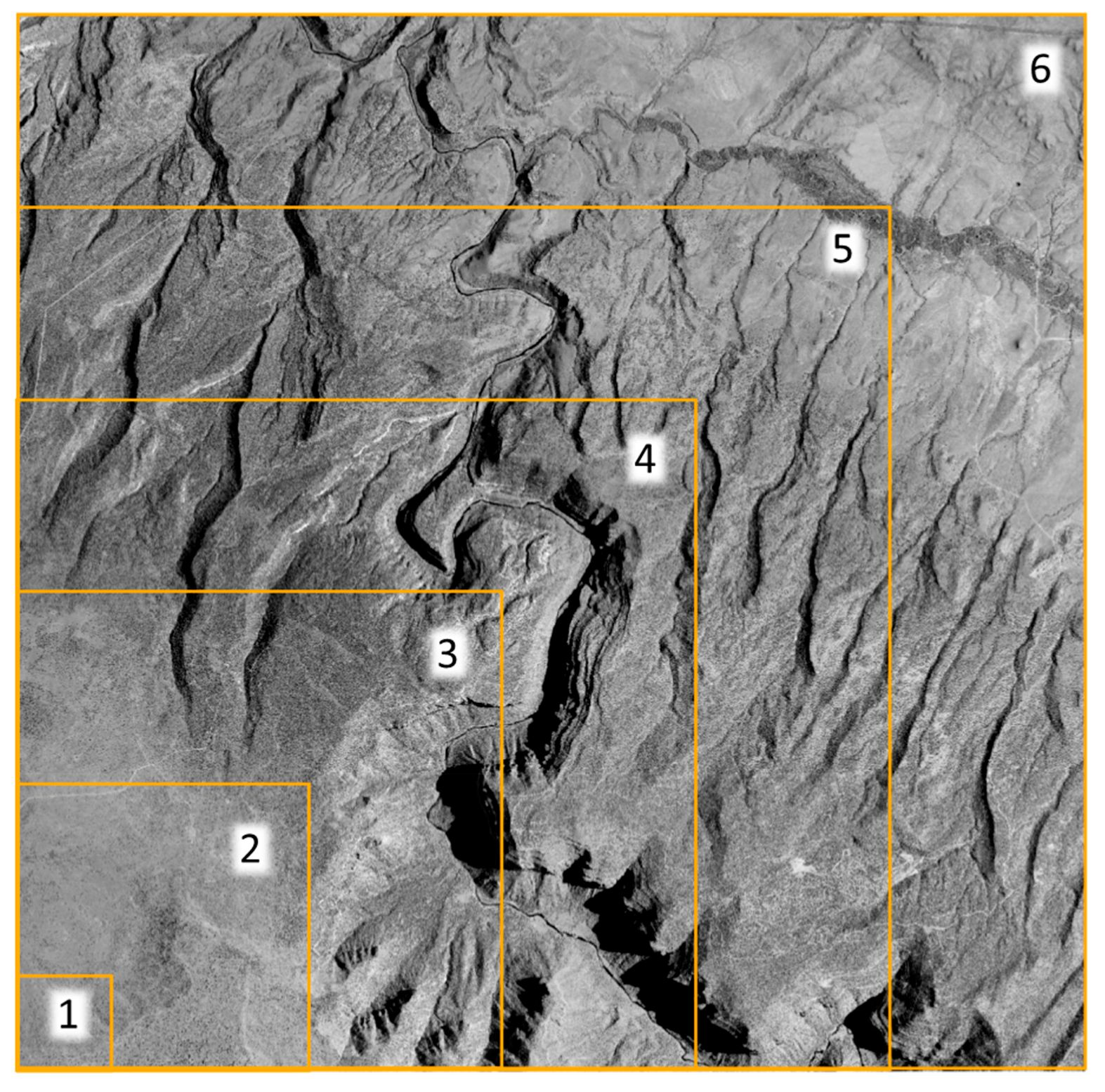
Figure 4.
Extent, size, and layout of each image within simulations.

Figure 5.
Conventional modeling (CM, blue) and function modeling (FM, yellow) regression results for processing time.
Figure 5.
Conventional modeling (CM, blue) and function modeling (FM, yellow) regression results for processing time.

Figure 6.
Conventional modeling (CM, blue) and function modeling (FM, yellow) regression results for storage space.
Figure 6.
Conventional modeling (CM, blue) and function modeling (FM, yellow) regression results for storage space.
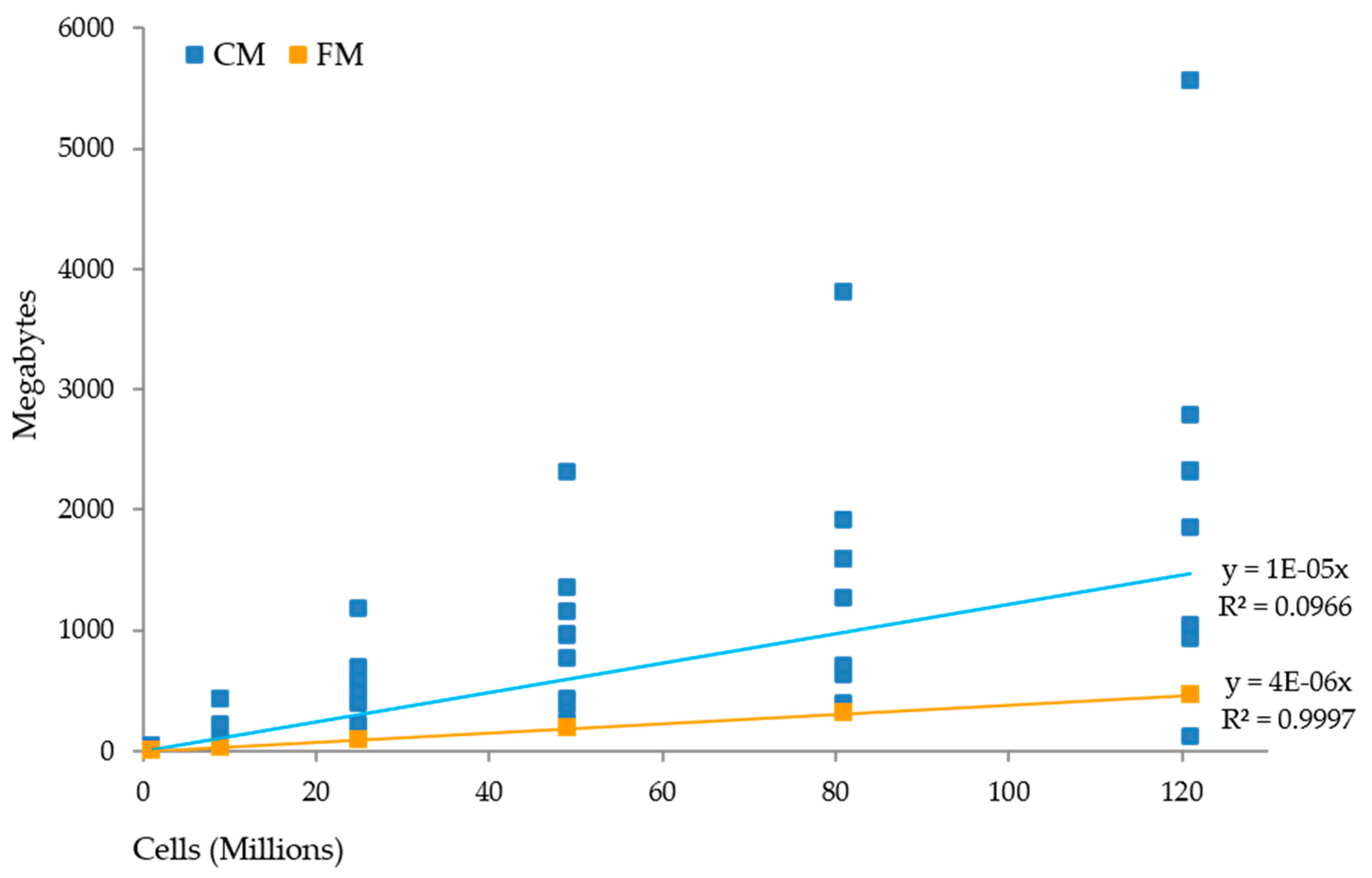
Figure 7.
Conventional modeling (CM) and function modeling (FM) processing time for a focal mean procedure performed on images of varying sizes (cells) using five different neighborhood window sizes.
Figure 7.
Conventional modeling (CM) and function modeling (FM) processing time for a focal mean procedure performed on images of varying sizes (cells) using five different neighborhood window sizes.
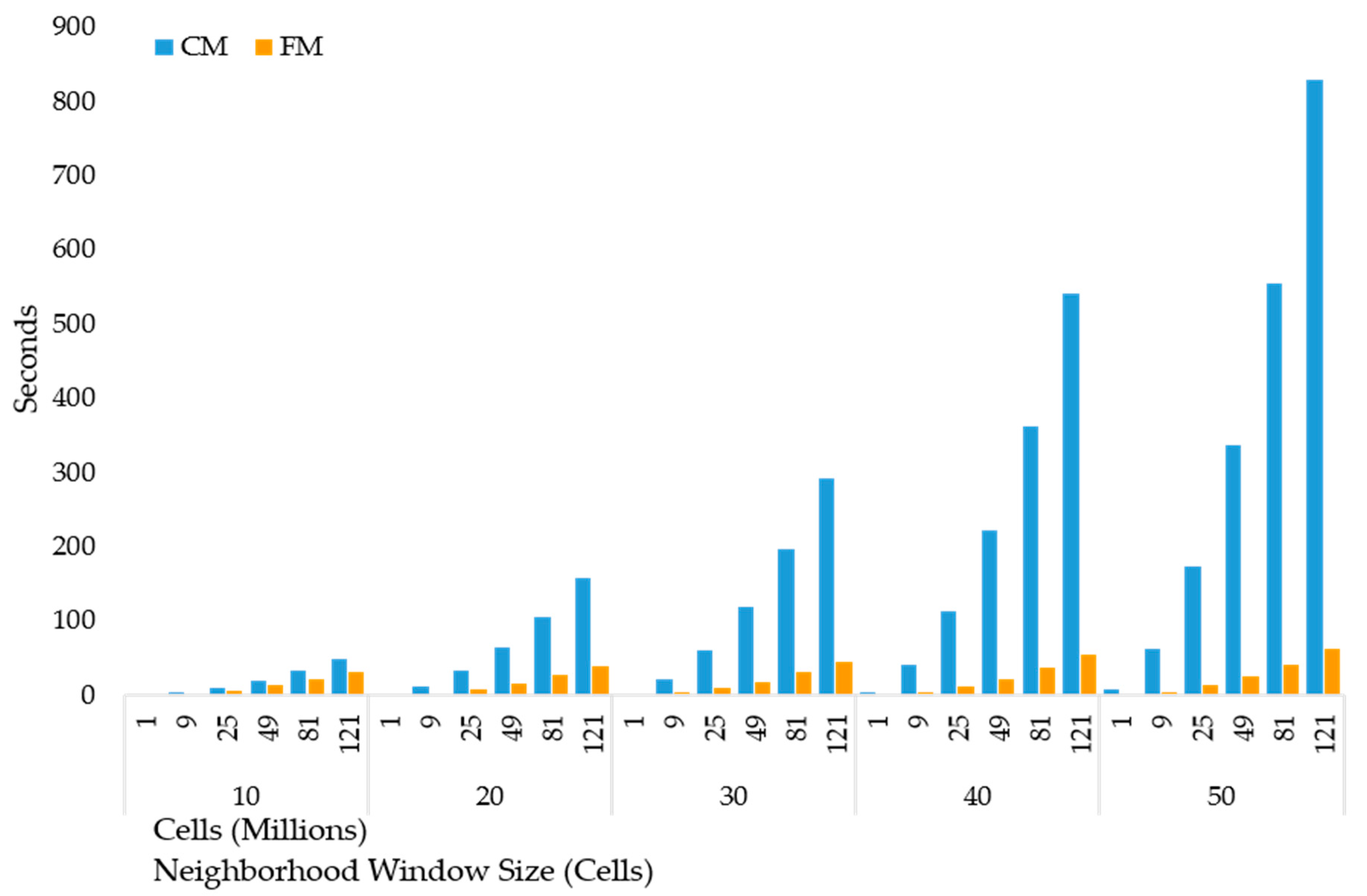
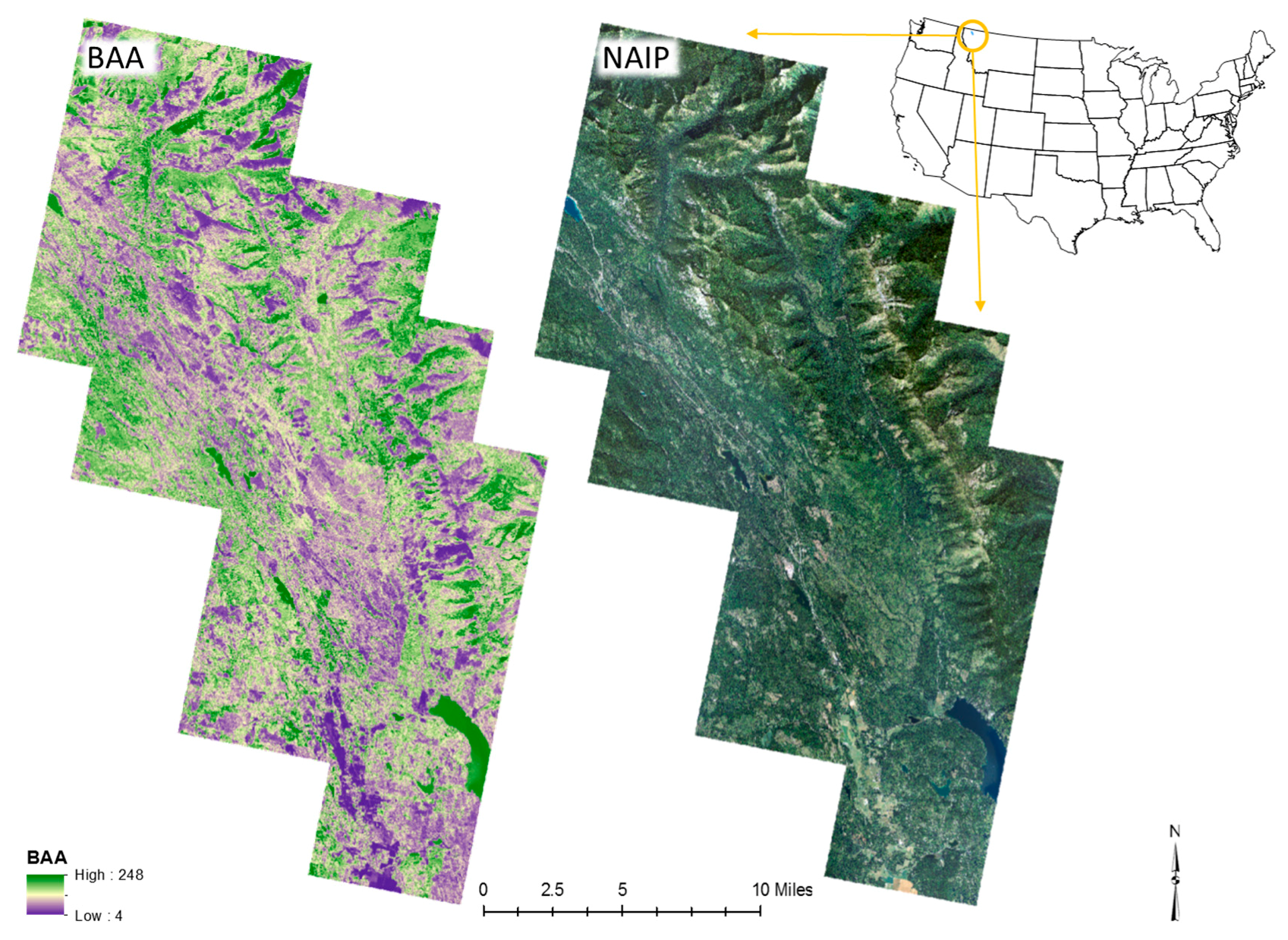
Figure 8.
Example of a basal area per acre (BAA) surface created using variable radius plots, National Agricultural Imagery Program (NAIP) image texture, and a random forest algorithm within FM. As areas transition from low to high BAA, colors transition from purple to green in the BAA graphic. Note, only forested areas are represented in the modeled outputs. Non-forested areas such as water in the southeastern portion of the NAIP imagery were not used to train the random forest model and do not accurately reflect BAA in the modeled outputs.

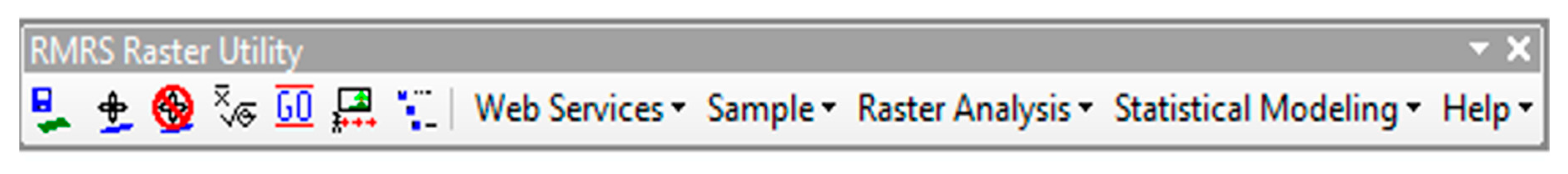
Figure 9.
The RMRS Raster Utility toolbar is a free, public source, object oriented library packaged as an ESRI add-in that simplifies data acquisition, raster sampling, and statistical and spatial modeling, while reducing the processing time and storage space associated with raster analysis.
Figure 9.
The RMRS Raster Utility toolbar is a free, public source, object oriented library packaged as an ESRI add-in that simplifies data acquisition, raster sampling, and statistical and spatial modeling, while reducing the processing time and storage space associated with raster analysis.


Table 1.
The 12 models and their spatial operations used to compare and contrast function modeling and conventional raster modeling in the simulations. Model number (column 1) also indicates the total number of processes performed for a given model. Each of the six simulations included processing all 12 models on increasingly large data sets.
| Model/Total Operations | Type and Number of Spatial Operations | ||||||
|---|---|---|---|---|---|---|---|
| Arithmetic, Add (+) | Arithmetic, Multiply (*) | Logical (≥) | Focal (Mean 7,7) | Conditional (True/False) | Convolution (Sum, 5,5) | Local (Sum ∑) | |
| 1 | 1 | - | - | - | - | - | - |
| 2 | 1 | 1 | - | - | - | - | - |
| 3 | 1 | 1 | 1 | - | - | - | - |
| 4 | 2 | 1 | 1 | - | - | - | - |
| 5 | 2 | 1 | 1 | 1 | - | - | - |
| 6 | 2 | 2 | 1 | 1 | - | - | - |
| 7 | 2 | 2 | 1 | 1 | 1 | - | - |
| 8 | 3 | 2 | 1 | 1 | 1 | - | - |
| 9 | 3 | 2 | 1 | 1 | 1 | 1 | - |
| 10 | 3 | 3 | 1 | 1 | 1 | 1 | - |
| 11 | 3 | 3 | 1 | 1 | 1 | 1 | 1 |
| 12 | 4 | 3 | 1 | 1 | 1 | 1 | 1 |
© 2017 by the authors. Licensee MDPI, Basel, Switzerland. This article is an open access article distributed under the terms and conditions of the Creative Commons Attribution (CC BY) license (http://creativecommons.org/licenses/by/4.0/).
Share and Cite
MDPI and ACS Style
Hogland, J.; Anderson, N. Function Modeling Improves the Efficiency of Spatial Modeling Using Big Data from Remote Sensing. Big Data Cogn. Comput. 2017, 1, 3. https://doi.org/10.3390/bdcc1010003
AMA Style
Hogland J, Anderson N. Function Modeling Improves the Efficiency of Spatial Modeling Using Big Data from Remote Sensing. Big Data and Cognitive Computing. 2017; 1(1):3. https://doi.org/10.3390/bdcc1010003
Chicago/Turabian StyleHogland, John, and Nathaniel Anderson. 2017. "Function Modeling Improves the Efficiency of Spatial Modeling Using Big Data from Remote Sensing" Big Data and Cognitive Computing 1, no. 1: 3. https://doi.org/10.3390/bdcc1010003