Relation between Observed and Perceived Traffic Noise and Socio-Economic Status in Urban Blocks of Different Characteristics

 , ,
, ,
Abstract
:1. Introduction
- (1)
- Which socio-economic groups mainly live in noisy locations (when looking at small-scale residential areas)?
- (2)
- Is there a correlation between noise exposure and the subjective perception of this stressor?
- (3)
- Is there a relation between perception of traffic noise and socio-economic characteristics?
2. Conceptual Issues of Environmental Justice and Noise Exposure in Urban Areas
2.1. Theoretical Approaches to Environmental Justice
2.2. Noise as Major Urban Stressor
2.3. Methodological Considerations and Recent Studies on Noise
- boundary effects: EJ studies often either use public statistical units (such as census blocks or ZIP code areas) or buffers around the origin of environmental stress factors (circular for point sources, linear for e.g., roads) to define the populations affected, which can lead to incorrect assignment of affected population [48,49]. We address this by using the results of a noise propagation model coupled with measurements and furthermore only comparing differences in affectedness among households living within our chosen study areas.
- Modifiable areal unit problem: The areal unit chosen for spatial analysis has repeatedly also been flagged as a potential source of uncertainty in EJ studies as the strength of association between socioeconomic and environmental variables often changes with scale. This phenomenon is known as the Modifiable Areal Unit Problem (MAUP). For instance, Mennis, Schweitzer and Stephenson (Jr.) illustrated the MAUP phenomenon by showing how using larger U.S. census- or ZIP code-based units show obscure variations and differences existing between smaller-scale units [50,51]. In this study we use socio-economic data from a household questionnaire which is not aggregated to larger units. The noise data originates from a dispersion model, which depicts dB(A) for 10 × 10 m raster cells. We thus do not consider MAUP to be a problem.
- Spatial autocorrelation is another important consideration in EJ analysis. According to Tobler’s first law of geography “(...) everything is related to everything else, but near things are more related than distant things” [52], such correlations can be expected in EJ analyses, which are based on the assumption that neither environmental burdens nor the population are randomly or evenly distributed in space. Spatial autocorrelation generally renders the application of general linear regression models inappropriate, since they rely on the assumption of independent residuals. However, in this study we test for correlations using Spearman’s Rho which is non-parametric.
3. Materials and Methodology
3.1. Study Areas and Data Acquisition
3.2. Measuring and Modeling of Noise
3.2.1. Noise Measurements
3.2.2. Noise Map
3.3. Software Used and Modelling Approach
3.3.1. Statistical Analyses
3.3.2. Socio-Economic Analyses
3.3.3. Spatial Analyses
4. Results
4.1. Description of the Survey Sample
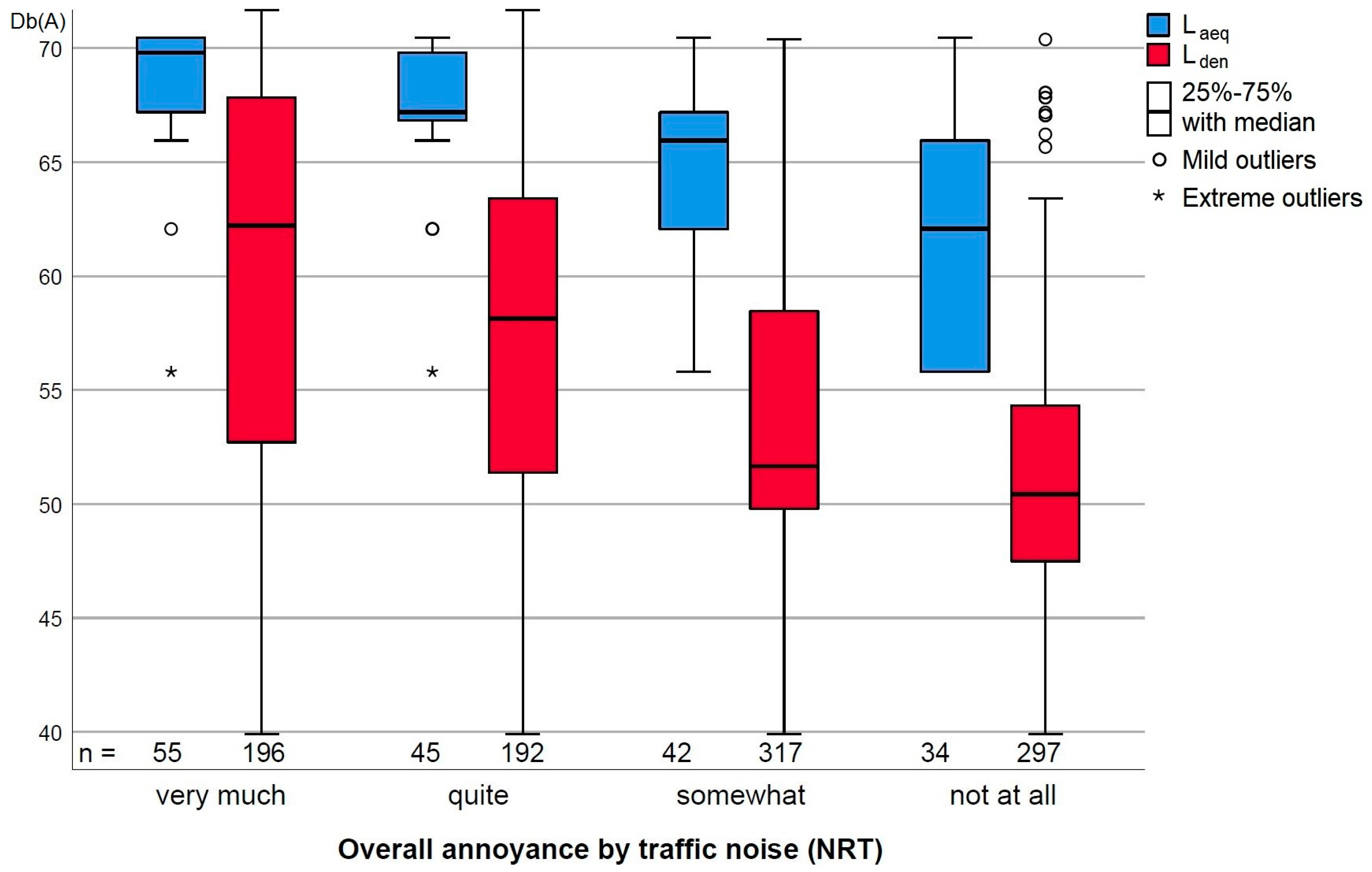
4.2. Noise Pollution and Perception
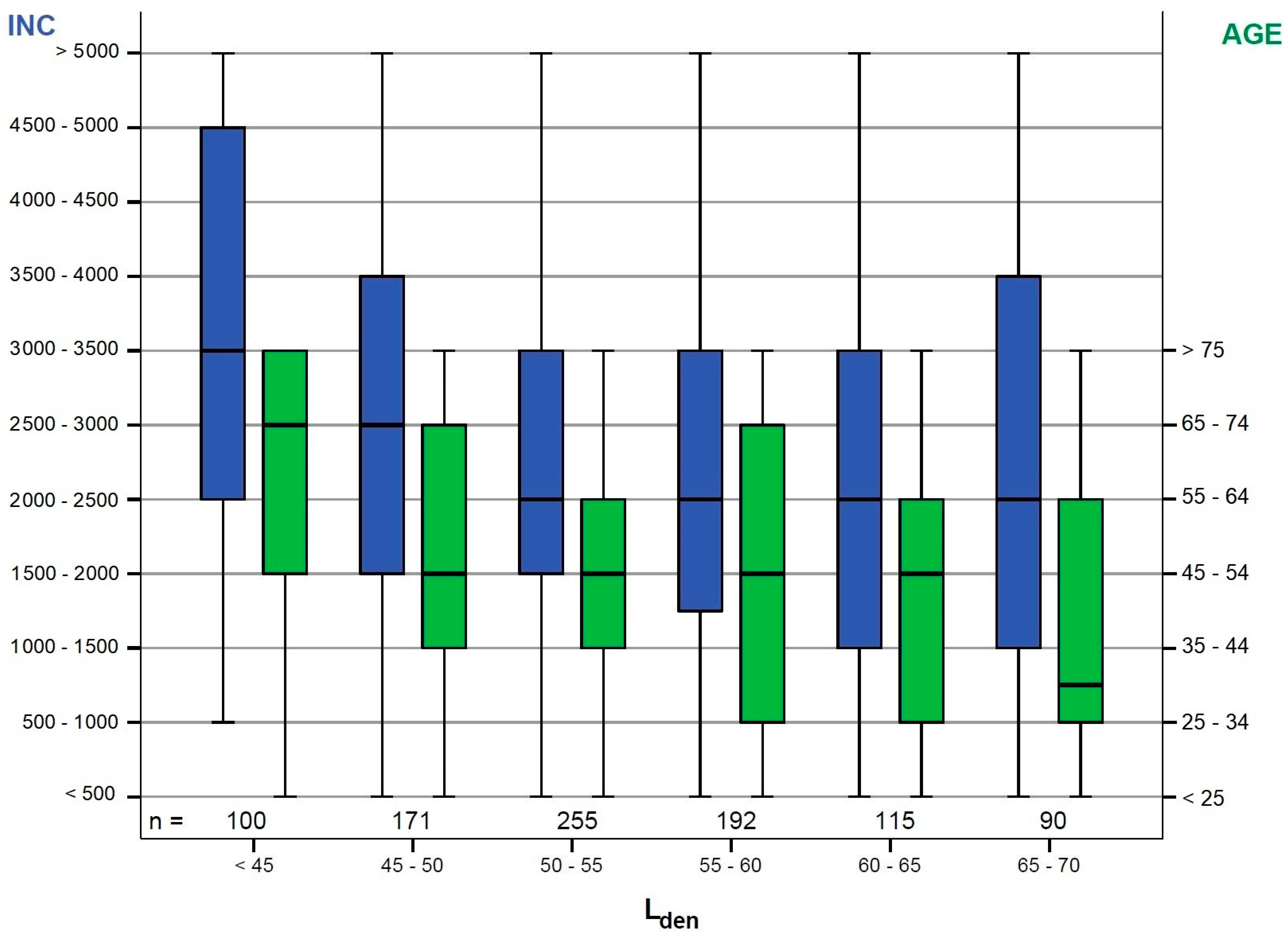
4.3. Noise Pollution and Socio-Economic Parameters
4.4. Noise Perception and Socio-Economic Parameters
5. Discussion, Conclusions and Outlook
Acknowledgments
Author Contributions
Conflicts of Interest
References
- Pulido, L. Flint, Environmental Racism, and Racial Capitalism. Capital. Nat. Social. 2016, 27, 1–16. [Google Scholar] [CrossRef]
- Erhart, M.; Hering, R.; Schulz, M.; Graf von Stillfried, D. Morbiditaetsatlas Hamburg: Gutachten zum Kleinräumigen Versorgungsbedarf in Hamburg; Erstellt Durch das Zentralinstitut für die kassenärztliche Versorgungin Deutschland im Auftrag der Behörde für Gesundheit und Verbraucherschutz Hamburg: Hamburg, Germany, 2013. [Google Scholar]
- Wing, S. Science for Reducing Health Inequalities Emerges from Social Justice Movements. New Solut. 2016, 26, 103–114. [Google Scholar] [CrossRef] [PubMed]
- Bullard, R.D. Unequal Protection. Environmental Justice and Communities of Color; Sierra Club Books: San Francisco, CA, USA, 1994. [Google Scholar]
- James, W.; Jia, C.; Kedia, S. Uneven magnitude of disparities in cancer risks from air toxics. Int. J. Environ. Res. Public Health 2012, 9, 4365–4385. [Google Scholar] [CrossRef] [PubMed]
- Bullard, R.D. Solid Waste Sites and the Black Houston Community. Sociol. Inq. 1983, 53, 273–288. [Google Scholar] [CrossRef] [PubMed]
- Maschewsky, W. Umweltgerechtigkeit, Public Health und Soziale Stadt; VAS Verlag für Akademische Schriften: Frankfurt, Germany, 2001. [Google Scholar]
- Maschewsky, W. Umweltgerechtigkeit. Gesundheitsrelevanz und Empirische Erfassung; Wissenschaftszentrum Berlin für Sozialforschung (WZB): Berlin, Germany, 2004. [Google Scholar]
- Umweltbundesamt. Umweltgerechtigkeit—Umwelt, Gesundheit und Soziale Lage. Available online: https://www.umweltbundesamt.de/themen/gesundheit/umwelteinfluesse-auf-den-menschen/umweltgerechtigkeit-umwelt-gesundheit-soziale-lage (accessed on 23 January 2018).
- Evans, G.W. The built environment and mental health. J. Urban Health Bull. N. Y. Acad. Med. 2003, 80, 536–555. [Google Scholar] [CrossRef] [PubMed]
- Lee, C. Environmental justice: Building a unified vision of health and the environment. Environ. Health Perspect. 2002, 110, 141–144. [Google Scholar] [CrossRef] [PubMed]
- Brulle, R.J.; Pellow, D.N. Environmental justice: Human health and environmental inequalities. Annu. Rev. Public Health 2006, 27, 103–124. [Google Scholar] [CrossRef] [PubMed]
- Taylor, W.C.; Floyd, M.F.; Whitt-Glover, M.C.; Brooks, J. Environmental justice: A framework for collaboration between the public health and parks and recreation fields to study disparities in physical activity. J. Phys. Act. Health 2007, 4, 50–63. [Google Scholar] [CrossRef]
- Bolte, G.; Mielck, A. Die soziale Verteilung von Umweltbelastungen: Neue Impulse für Public Health Forschung und Praxis. In Umweltgerechtigkeit: Die Soziale Verteilung von Umweltbelastungen; Bolte, G., Ed.; Juventa: Weinheim, München, 2004; pp. 7–28. [Google Scholar]
- Walker, G.P. Environmental Justice. Concepts, Evidence and Politics; Routledge: London, UK, 2012. [Google Scholar]
- Holifield, R. Environmental justice and political ecology. In The Routledge Handbook of Political Ecology, 1st ed.; Perreault, T., Bridge, G., McCarthy, J., Eds.; Routledge: London, UK, 2015; pp. 585–597. [Google Scholar]
- Young, I.M. Justice and the Politics of Difference; Paperback Reissue [Electronic Version]; Princeton University Press: Princeton, NJ, USA, 2011. [Google Scholar]
- Bolte, G.; Bunge, C.; Hornberg, C.; Köckler, H.; Mielck, A. (Eds.) Umweltgerechtigkeit. Chancengleichheit bei Umwelt und Gesundheit: Konzepte, Datenlage und Handlungsperspektiven, 1st ed.; Verlag H. Huber: Bern, Switzerland, 2012. [Google Scholar]
- Preisendörfer, P. Umweltgerechtigkeit: Von sozial-räumlicher Ungleichheit hin zu postulierter Ungerechtigkeit lokaler Umweltbelastungen. Soziale Welt 2014, 65, 25–45. [Google Scholar] [CrossRef]
- Kohlhuber, M.; Mielck, A.; Weiland, S.K.; Bolte, G. Social inequality in perceived environmental exposures in relation to housing conditions in Germany. Environ. Res. 2006, 101, 246–255. [Google Scholar] [CrossRef] [PubMed]
- Von Szombathely, M.; Albrecht, M.; Antanaskovic, D.; Augustin, J.; Augustin, M.; Bechtel, B.; Bürk, T.; Fischereit, J.; Grawe, D.; Hoffmann, P.; et al. A Conceptual Modeling Approach to Health-Related Urban Well-Being. Urban Sci. 2017, 1, 17. [Google Scholar] [CrossRef]
- Babisch, W.; Wolf, K.; Petz, M.; Heinrich, J.; Cyrys, J.; Peters, A. Associations between Traffic Noise, Particulate Air Pollution, Hypertension, and Isolated Systolic Hypertension in Adults: The KORA Study. Environ. Health Perspect. 2014, 122, 492–498. [Google Scholar] [CrossRef] [PubMed]
- Van Kempen, E.; Babisch, W. The quantitative relationship between road traffic noise and hypertension. J. Hypertens. 2012, 30, 1075–1086. [Google Scholar] [CrossRef] [PubMed]
- Ising, H.; Babisch, W.; Kruppa, B. Noise-induced endocrine effects and cardiovascular risk. Noise Health 1999, 1, 37–48. [Google Scholar] [PubMed]
- Bockelbrink, A.; Willich, S.N.; Dirzus, I.; Reich, A.; Lau, S.; Wahn, U.; Keil, T. Environmental Noise and Asthma in Children: Sex-Specific Differences. J. Asthma 2008, 45, 770–773. [Google Scholar] [CrossRef] [PubMed]
- Duhme, H.; Weiland, S.K.; Keil, U.; Kraemer, B.; Schmid, M.; Stender, M.; et al. The association between self-reported symptoms of asthma and allergic rhinitis and self-reported traffic density on street of residence in adolescents. Epidemiology 1996, 7, 578–582. [Google Scholar] [CrossRef] [PubMed]
- Ising, H.; Lange-Asschenfeldt, H.; Lieber, G.F.; Weinhold, H.; Eilts, M. Effects of long-term exposure to street traffic exhaust on the development of skin and respiratory tract diseases in children. Schriftenr. Ver. Wasser Boden Lufthyg. 2003, 112, 81–99. [Google Scholar]
- Casey, J.A.; Morello-Frosch, R.; Mennitt, D.J.; Fristrup, K.; Ogburn, E.L.; James, P. Race/ethnicity, socioeconomic status, residential segregation, and spatial variation in noise exposure in the contiguous United States. Environ. Health Perspect. 2017, 125, 077017. [Google Scholar] [CrossRef] [PubMed]
- Federal Republic of Germany. Sechste Allgemeine Verwaltungsvorschrift zum Bundes-Immissionsschutzgesetz (Technische Anleitung zum Schutz Gegen Lärm—TA Lärm); TA Lärm; Federal Republic of Germany: Bonn, Germany, 1998.
- Federal Republic of Germany. Sechzehnte Verordnung zur Durchführung des Bundes-Immissionsschutzgesetzes (Verkehrslärmschutzverordnung—16. BImSchV); 16. BImSchV; Federal Republic of Germany: Bonn, Germany, 1990.
- Carrier, M.; Apparicio, P.; Seguin, A.M. Road traffic noise in Montreal and environmental equity: What is the situation for the most vulnerable population groups? J. Transp. Geogr. 2016, 51, 1–8. [Google Scholar] [CrossRef]
- Becker, T. Sozialräumliche Verteilung von Verkehrsbedingtem Lärm und Luftschadstoffen am Beispiel von Berlin; Technische Universität Dresden: Dresden, Germany, 2016. [Google Scholar]
- Dale, L.M.; Goudreau, S.; Perron, S.; Ragettli, M.S.; Hatzopoulou, M.; Smargiassi, A. Socioeconomic status and environmental noise exposure in Montreal, Canada. BMC Public Health 2015, 15, 1–8. [Google Scholar] [CrossRef] [PubMed]
- Riedel, N.; Scheiner, J.; Müller, G.; Köckler, H. Assessing the relationship between objective and subjective indicators of residential exposure to road traffic noise in the context of environmental justice. J. Environ. Plan. Manag. 2014, 57, 1398–1421. [Google Scholar] [CrossRef]
- Lakes, T.; Brückner, M. Socio-spatial Distribution of Noise Exposure in Berlin. In Environmental Justice, II. Special Issue; Federal Environmental Agency: Berlin, Germany, 2011. [Google Scholar]
- Havard, S.; Reich, B.J.; Bean, K.; Chaix, B. Social inequalities in residential exposure to road traffic noise: An environmental justice analysis based on the RECORD Cohort Study. Occup. Environ. Med. 2011, 68, 366–374. [Google Scholar] [CrossRef] [PubMed]
- Bocquier, A.; Cortaredona, S.; Boutin, C.; David, A.; Bigot, A.; Chaix, B.; Gaudart, J.; Verger, P. Small-area analysis of social inequalities in residential exposure to road traffic noise in Marseille, France. Eur. J. Public Health 2012, 23, 540–546. [Google Scholar] [CrossRef] [PubMed]
- Schweitzer, L.; Valenzuela, A. Environmental injustice and transportation: The claims and the evidence. J. Plan. Lit. 2004, 18, 383–398. [Google Scholar] [CrossRef]
- Senatsverwaltung für Stadtentwicklung und Wohnen. Umweltatlas Berlin. Available online: http://www.stadtentwicklung.berlin.de/umwelt/umweltatlas/index.shtml (accessed on 23 January 2018).
- Lakes, T.; Brückner, M.; Krämer, A. Development of an environmental justice index to determine socio-economic disparities of noise pollution and green space in residential areas in Berlin. J. Environ. Plan. Manag. 2014, 57, 538–556. [Google Scholar] [CrossRef]
- Flacke, J.; Schüle, S.A.; Köckler, H.; Bolte, G. Mapping Environmental Inequalities Relevant for Health for Informing Urban Planning Interventions: A Case Study in the City of Dortmund, Germany. Int. J. Environ. Res. Public Health 2016, 13, 711. [Google Scholar] [CrossRef] [PubMed]
- Cesaroni, G.; Badaloni, C.; Romano, V.; Donato, E.; Perucci, C.A.; Forastiere, F. Socioeconomic position and health status of people who live near busy roads: The Rome Longitudinal Study (RoLS). Environ. Health 2010, 41, 1–12. [Google Scholar] [CrossRef] [PubMed]
- Kohlhuber, M.; Heinrich, J.; Van Den Hazel, P.; Zuurbier, M.; Bistrup, M.L.; Koppe, J.G.; Bolte, G. Children’s environmental health: Why should social disparities be considered? Acta Pædiatrica 2016, 95, 26–30. [Google Scholar] [CrossRef] [PubMed]
- Oiamo, T.H.; Davies, H.; Rinner, C. Environmental Noise Study in the City of Toronto; City of Toronto Public Health Project: Toronto, ON, Canada, 2017. [Google Scholar]
- Nega, T.H.; Chihara, L.; Smith, K.; Jayaraman, M. Traffic noise and inequality in the twin cities, Minnesota. Hum. Ecol. Risk Assess. Int. J. 2013, 19, 601–619. [Google Scholar] [CrossRef]
- Lam, K.-C.; Chan, P.-K. Socio-economic status and inequalities in exposure to transportation noise in Hong Kong. Transportation 2006, 2, 107–113. [Google Scholar] [CrossRef]
- Moreno-Jiménez, A.; Cañada-Torrecilla, R.; Vidal-Domínguez, M.J.; Palacios-García, A.; Martínez-Suárez, P. Assessing environmental justice through potential exposure to air pollution: A socio-spatial analysis in Madrid and Barcelona, Spain. Geoforum 2016, 69, 117–131. [Google Scholar] [CrossRef]
- Bowen, W. An Analytical Review of Environmental Justice Research: What Do We Really Know? Environ. Manag. 2002, 29, 3–15. [Google Scholar] [CrossRef]
- Brender, J.D.; Maantay, J.A.; Chakraborty, J. Residential Proximity to Environmental Hazards and Adverse Health Outcomes. Am. J. Public Health 2011, 101, S37–S52. [Google Scholar] [CrossRef] [PubMed]
- Mennis, J. Using geographic information systems to create and analyze statistical surfaces of population and risk for environmental justice analysis. Soc. Sci. Q. 2002, 83, 281–297. [Google Scholar] [CrossRef]
- Schweitzer, L.A.; Stephenson, M., Jr. Right Answers, Wrong Questions: Environmental Justice as Urban Research. Urban Stud. 2007, 44, 319–337. [Google Scholar] [CrossRef]
- Tobler, W.R. A Computer Movie Simulating Urban Growth in the Detroit Region. Econ. Geogr. 1970, 46, 234–240. [Google Scholar] [CrossRef]
- BSU—Behörde für Stadtentwicklung und Umwelt. Strategische Lärmkarte Straßenverkehr Lnight. Available online: http://www.hamburg.de/contentblob/3476532/data/lnight-strasse-2012.pdf (accessed on 23 January 2018).
- BSU—Behörde für Stadtentwicklung und Umwelt. Strategische Lärmkarte Straßenverkehr Lden. Available online: http://www.hamburg.de/contentblob/3476512/data/lden-strasse-2012.pdf (accessed on 23 January 2018).
- Bolte, G.; Kohlhuber, M. Untersuchungen zur Ökologischen Gerechtigkeit: Explorative Vorbereitungsstudie. Teilprojekt A: Systematische Zusammenstellung der Datenlage in Deutschland; Umweltforschungsplan 3707 17 102/01; Umweltbundesamt (UBA): Dessau-Roßlau, Germany, 2008. [Google Scholar]
- Hornberg, C.; Bunge, C.; Pauli, A. Strategien für Mehr Umweltgerechtigkeit. Handlungsfelder für Forschung und Praxis; Universität Bielefeld: Bielefeld, Germany, 2011. [Google Scholar]
- Bunge, C. Umweltgerechtigkeit. Soziale und Räumliche Verteilung Gesundheitsrelevanter Umweltbelastungen und -Ressourcen; Verlang H. Huber: Bern, Germany, 2013. [Google Scholar]
- Köckler, H. Umweltbezogene Gerechtigkeit und Immissionsbelastungen am Beispiel der Stadt Kassel; Kassel Univ. Press: Kassel, Germany, 2008. [Google Scholar]
- Baranzini, A.; Schaerer, C.; Thalmann, P. Using measured instead of perceived noise in hedonic models. Transp. Res. Part D Transp. Environ. 2010, 15, 473–482. [Google Scholar] [CrossRef]
- Gaffron, P. Urban transport, environmental justice and human daily activity patterns. Trans. Policy 2012, 20, 114–127. [Google Scholar] [CrossRef]
- Balestroni, G.; Bertolotti, G. L’EuroQol-5D (EQ-5D): Uno strumento per la misura della qualità della vita. Monaldi Arch. Chest Dis. 2012, 78, 155–159. [Google Scholar] [CrossRef] [PubMed]
- Feng, Y.; Parkin, D.; Devlin, N.J. Assessing the performance of the EQ-VAS in the NHS PROMs programme. Qual. Life Res. 2014, 23, 977–989. [Google Scholar] [CrossRef] [PubMed]
- Diekmann, A.; Jann, B. Anreizformen und Ausschöpfungsquoten bei postalischen Befragungen: Eine Prüfung der Reziprozitätshypothese. ZUMA Nachr. 2001, 48, 18–27. [Google Scholar]
- Petermann, S. Rücklauf und systematische Verzerrungen bei postalischen Befragungen: Eine Analyse der Bürgerumfrage Halle 2003. ZUMA Nach. 2005, 57, 55–78. [Google Scholar]
- League of American Bicyclists. Bicycle Account Guidelines. 2013. Available online: http://bikeleague.org/sites/default/files/Bicycle_Account_Guidelines.pdf (accessed on 23 January 2018).
- New South Wales Government. Adult Population Health Survey. Forthcoming. Available online: http://www.health.nsw.gov.au/surveys/adult/Pages/default.aspx (accessed on 23 January 2018).
- Universitätsklinikum Hamburg-Eppendorf. Hamburg City Health Study. Available online: http://hchs.hamburg/ (accessed on 23 January 2018).
- Schuster, C.; Honold, J.; Lauf, S.; Lakes, T. Urban heat stress: Novel survey suggests health and fitness as future avenue for research and adaptation strategies. Environ. Res. Lett. 2017, 12, 44021. [Google Scholar] [CrossRef]
- Bechtel, B.; Schmidt, K. Floristic mapping data as a proxy for the mean Urban heat Island. Clim. Res. 2011, 49, 45–58. [Google Scholar] [CrossRef]
- Boettcher, M.; Flagg, D.D.; Grawe, D.; Hoffmann, P.; Petrik, R.; Schlünzen, K.H.; Schoetter, R.; Teichert, N. Modelling impacts of urban developments and climate adaptation measures on summer climate of Hamburg. Urban Sci. 2018. submitted. [Google Scholar]
- Stewart, I.D.; Oke, T.R. Local Climate Zones for Urban Temperature Studies. Bull. Am. Meteor. Soc. 2012, 93, 1879–1900. [Google Scholar] [CrossRef]
- Kaveckis, G. Modeling Future Populations Vulnerability to Heat Waves in Greater Hamburg; Universität Hamburg: Hamburg, Germany, 2017. [Google Scholar]
- Karten, T. GEWOS Institut für Stadt-, Regional- und Wohnungsforschung GmbH; Sozialmonitoring Integrierte Stadtteilentwicklung: Hamburg, Germany, 2017. [Google Scholar]
- ISO. Acoustics—Assessment of Noiseannoyance by Means of Social and Socio-Acoustic Surveys. Available online: https://www.iso.org/standard/28630.html (accessed on 23 January 2018).
- Heimann, D. Schallausbreitung unter Meteorologischen und Topografischen Gegebenheiten; Deutsches Zentrum für Luft- und Raumfahrt: Hamburg, Germany, 2003. [Google Scholar]
- Müller, G.; Möser, M. Taschenbuch der Technischen Akustik; Springer: Berlin, Germany, 2004. [Google Scholar]
- Piercy, J.E.; Embleton, T.F.; Sutherland, L.C. Review of noise propagation in the atmosphere. J. Acoust. Soc. Am. 1977, 61, 1403–1418. [Google Scholar] [CrossRef] [PubMed]
- European Commission (EC). Directive 2002/49/EC of the European Parliament and of the Council of 25 June 2002 Relating to the Assessment and Management of Environmental Noise. Environmental Noise Directive; European Commission: Brussels, Belgium, 2002. [Google Scholar]
- Federal Republic of Germany. Bekanntmachung der Vorläufigen Berechnungsverfahren für den Umgebungslärm nach § 5 Abs. 1 der Verordnung über die Lärmkartierung (34. BImSchV); Federal Republic of Germany: Berlin, Germany, 2006.
- Schick, A. Schallbewertung. Grundlagen der Lärmforschung; Springer: Berlin/Heidelberg, Germany, 1990. [Google Scholar]
- Freie und Hansestadt Hamburg. Transparenzportal Hamburg. Available online: http://transparenz.hamburg.de/ (accessed on 23 January 2018).
- Mielck, A. Unterschiede bei Läarmbelastungen und Luftverschmutzungen nach dem Haushaltseinkommen. In Umweltgerechtigkeit. Die Soziale Verteilung von Umweltbelastungen; Bolte, G., Mielck, A., Eds.; Juventa: Weinheim, Germany, 2004; pp. 139–153. [Google Scholar]
- Empirica. Städte Mit den Höchsten Mietpreisen für Wohnungen in Deutschland im 4. Quartal 2017 (in Euro pro Quadratmeter). In Statista—Das Statistik-Portal. Available online: https://de.statista.com/statistik/daten/studie/1885/umfrage/mietpreise-in-den-groessten-staedten-deutschlands/ (accessed on 23 January 2018).
- Fyhri, A.; Klaeboe, R. Road traffic noise, sensitivity, annoyance and self-reported health—A structural equation model exercise. Environ. Int. 2009, 35, 91–97. [Google Scholar] [CrossRef] [PubMed]
- Nijland, H.A.; Hartemink, S.; van Kamp, I.; van Wee, B. The influence of sensitivity for road traffic noise on residential location: Does it trigger a process of spatial selection? J. Acoust. Soc. Am. 2007, 122, 1595. [Google Scholar] [CrossRef] [PubMed]
- Statistisches Amt für Hamburg und Schleswig-Holstein. Bevölkerung mit Migrationshintergrund in den Hamburger Stadtteilen Ende. 2016. Available online: https://www.statistik-nord.de/fileadmin/Dokumente/Statistik_informiert_SPEZIAL/SI_SPEZIAL_V_2017_Korrektur.pdf (accessed on 23 January 2018).
- Raddatz, L.; Mennis, J. Environmental Justice in Hamburg, Germany. Prof. Geogr. 2013, 65, 495–511. [Google Scholar] [CrossRef]
- Brainard, J.S.; Jones, A.P.; Bateman, I.J.; Lovett, A.A. Exposure to Environmental Urban Noise Pollution in Birmingham, UK. Urban Stud. 2016, 41, 2581–2600. [Google Scholar] [CrossRef]
- Fischer, M.M.; Getis, A. (Eds.) Handbook of Applied Spatial Analysis. Software Tools, Methods and Applications; Springer: Heidelberg, Germany, 2010. [Google Scholar]
- Statistisches Amt für Hamburg und Schleswig-Holstein. Lohn- und Einkommensstatistik in Hamburg 2013. 2017. Available online: https://www.statistik-nord.de/fileadmin/Dokumente/Statistik_informiert_SPEZIAL/SI_SPEZIAL_VIII_2017.pdf (accessed on 23 January 2018).
- Van Gerven, P.W.M.; Vos, H.; van Boxtel, M.P.J.; Janssen, S.A.; Miedema, H.M.E. Annoyance from environmental noise across the lifespan. J. Acoust. Soc. Am. 2009, 126, 187–194. [Google Scholar] [CrossRef] [PubMed]
- Häder, M. Empirische Sozialforschung, 2nd ed.; Überarbeitete Auflage; VS Verl. für Sozialwiss: Wiesbaden, Germany, 2010. [Google Scholar]
- Diekmann, A. Empirische Sozialforschung. Grundlagen, Methoden, Anwendungen; Rowohlt: Reinbek bei Hamburg, Germany, 2017. [Google Scholar]
- Van Kamp, I.; Davies, H. Noise and health in vulnerable groups: A review. Noise Health 2013, 15, 153–159. [Google Scholar] [CrossRef] [PubMed]
- Babisch, W.; Swart, W.; Houthuijs, D.; Selander, J.; Bluhm, G.; Pershagen, G.; Dimakopoulou, K.; Haralabidis, A.S.; Katsouyanni, K.; Davou, E.; et al. Exposure modifiers of the relationships of transportation noise with high blood pressure and noise annoyance. J. Acoust. Soc. Am. 2012, 132, 3788–3808. [Google Scholar] [CrossRef] [PubMed]
- Babisch, W.; Pershagen, G.; Selander, J.; Houthuijs, D.; Breugelmans, O.; Cadum, E.; Vigna-Taglianti, F.; Katsouyanni, K.; Haralabidis, A.S.; Dimakopoulou, K.; et al. Noise annoyance—A modifier of the association between noise level and cardiovascular health. Sci. Total Environ. 2013, 452–453, 50–57. [Google Scholar] [CrossRef] [PubMed]
- Miedema, H.M.E. Annoyance Caused by Environmental Noise: Elements for Evidence-Based Noise Policies. J. Soc. Issues 2007, 63, 41–57. [Google Scholar] [CrossRef]
- Meyer-Wellmann, J. Bürgerschaft Beschließt Massiven Wohnungsbau an Hauptstraßen. Hamburger Abendblatt. Available online: https://www.abendblatt.de/hamburg/article212208285/Buergerschaft-beschliesst-massiven-Wohnungsbau-an-Hauptstrassen.html (accessed on 11 October 2017).
- Asendorpf, D. (Interview) “Wenn Sie da Wohnen …” Zeit Online. Available online: http://www.zeit.de/2017/34/laerm-rainer-guski-lautstaerke (accessed on 16 August 2017).
- Yang, Z.; Wang, S. The impact of privatization of public housing on housing affordability in Beijing: An assessment using household survey data. Local Econ. 2011, 26, 384–400. [Google Scholar] [CrossRef]
- Lee, J.A. Rights at Risk in Privatized Public Housing. 2015. Available online: https://scholarworks.law.ubalt.edu/cgi/viewcontent.cgi?article=1391&context=all_fac (accessed on 23 January 2018).
- Twickel, C. Gentrifidingsbums. Oder Eine Stadt für Alle, 4th ed.; Nautilus: Hamburg, Germany, 2013. [Google Scholar]
- Davoudi, S.; Atkinson, R. Social Exclusion and the British Planning System. Plan. Pract. Res. 1999, 14, 225–236. [Google Scholar] [CrossRef]
- Walker, G.; Mitchell, G.; Fairburn, J.; Smith, G. Industrial pollution and social deprivation: Evidence and complexity in evaluating and responding to environmental inequality. Local Environ. 2007, 10, 361–377. [Google Scholar] [CrossRef] [Green Version]
- Cutter, S.L. Race, class and environmental justice. Prog. Hum. Geogr. 2016, 19, 111–122. [Google Scholar] [CrossRef]
- Speer, J. Henri Lefebvre: Spatial Politics, Everyday Life and the Right to the City. AAG Rev. Books 2015, 3, 4–5. [Google Scholar] [CrossRef]
- Martens, K. Transport Justice. Designing Fair Transportation Systems; Routledge: London, UK, 2016. [Google Scholar]
- Walker, G.; Bulkeley, H. Geographies of environmental justice. Geoforum 2006, 37, 655–659. [Google Scholar] [CrossRef] [Green Version]
- Forkenbrock, D.J.; Sheeley, J. Effective Methods for Environmental Justice Assessment; NCHRP Report No. 532; Transportation Research Board: Washington, DC, USA, 2004. [Google Scholar]
- Steven, H. Investigations on Noise Emission of Motor Vehicles in Road Traffic: Research Project 200 54 135; Final Report; RWTUEV Fahrzeug GmbH—Institute for Vehicle Technology: Wuerselen, Germany, 2005. [Google Scholar]
- Connolly Carmalt, J.; Faubion, T. Normative approaches to critical health geography. Prog. Hum. Geogr. 2010, 34, 292–308. [Google Scholar] [CrossRef]
- Stephens, C. Revisiting urban health and social inequalities: The devil is in the detail and the solution is in all of us. Environ. Urban. 2011, 23, 29–40. [Google Scholar] [CrossRef]
- Sicotte, D. Diversity and Intersectionality among Environmentally Burdened Communities in the Philadelphia Metropolitan Area, USA. Urban Stud. 2013, 51, 1850–1870. [Google Scholar] [CrossRef]
- Reckien, D.; Creutzig, F.; Fernandez, B.; Lwasa, S.; Tovar-Restrepo, M.; Mcevoy, D.; Satterthwaite, D. Climate change, equity and the Sustainable Development Goals: An urban perspective. Environ. Urban. 2017, 29, 159–182. [Google Scholar] [CrossRef]
- Walker, G. Environmental justice, impact assessment and the politics of knowledge: The implications of assessing the social distribution of environmental outcomes. Environ. Impact Assess. Rev. 2010, 30, 312–318. [Google Scholar] [CrossRef]


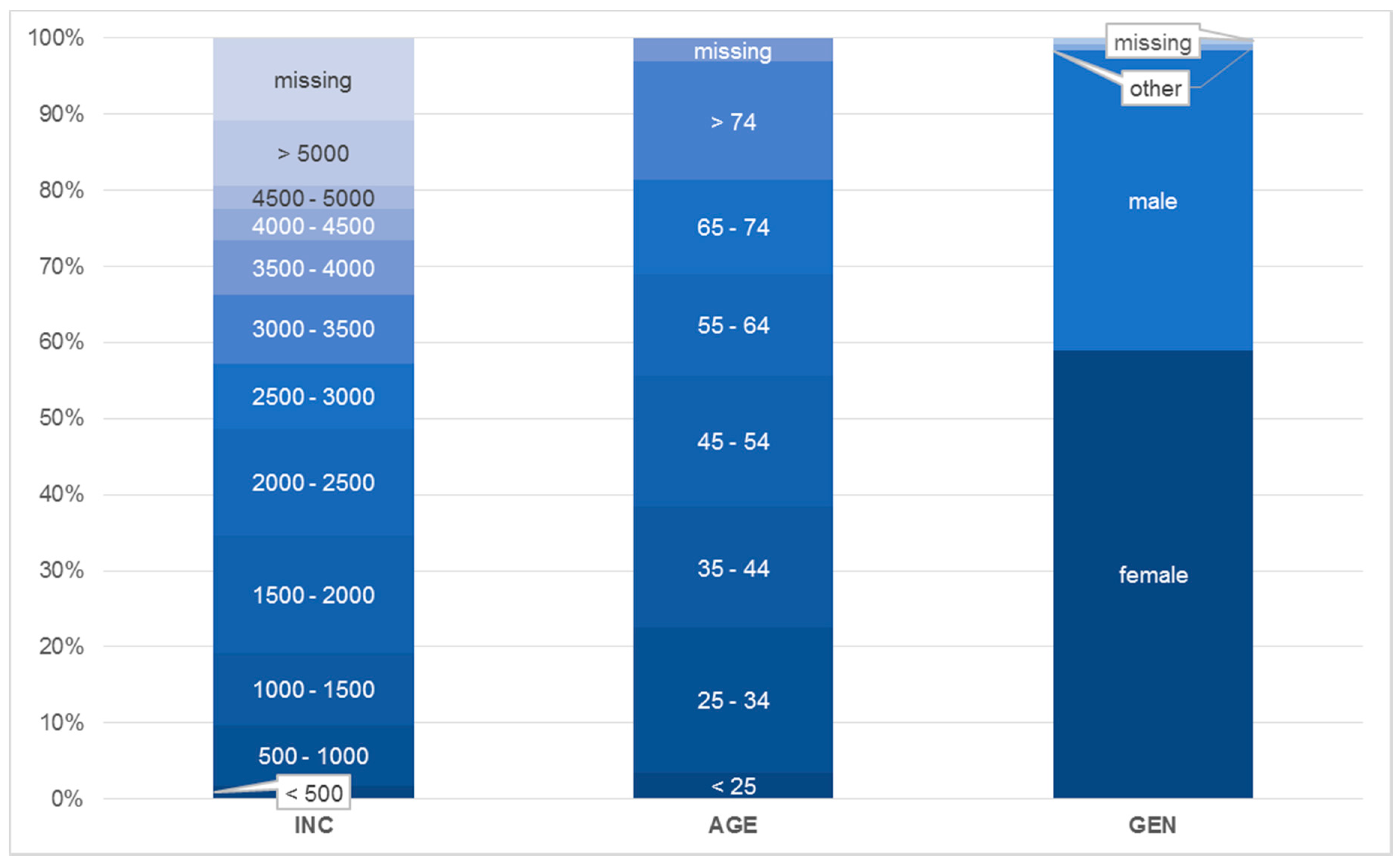
| Question | Variable | Answer scale | No. Cases (n) | |
|---|---|---|---|---|
| Do you feel disturbed by noise in your apartment/house? (noise of every kind) | …on weekdays | NWD | 4-level Likert (very much, quite, some-what, not at all) | 1036 |
| …on weekends | NWE | 1020 | ||
| …during night | NNI | 1022 | ||
| To what extent do you feel disturbed in your apartment/house by road traffic noise? | NRT | 4-level Likert (very much, quite, some-what, not at all) | 1002 | |
| How old are you? | AGE | open | 1048 | |
| What is the approximate monthly net income of your household? (Combined disposable income of all household members, incl. child support etc.) | INC | Eleven classes in 500 € steps; without limit from 5000 € up | 964 | |
| Highest level of education reached? | EDU | Five categories | 1057 | |
| What is/are your occupation(s)? (Multiple answers possible) | OCC | Seven categories, open answer | 1047 | |
| Gender? | GEN | Three categories (incl. other) | 1073 | |
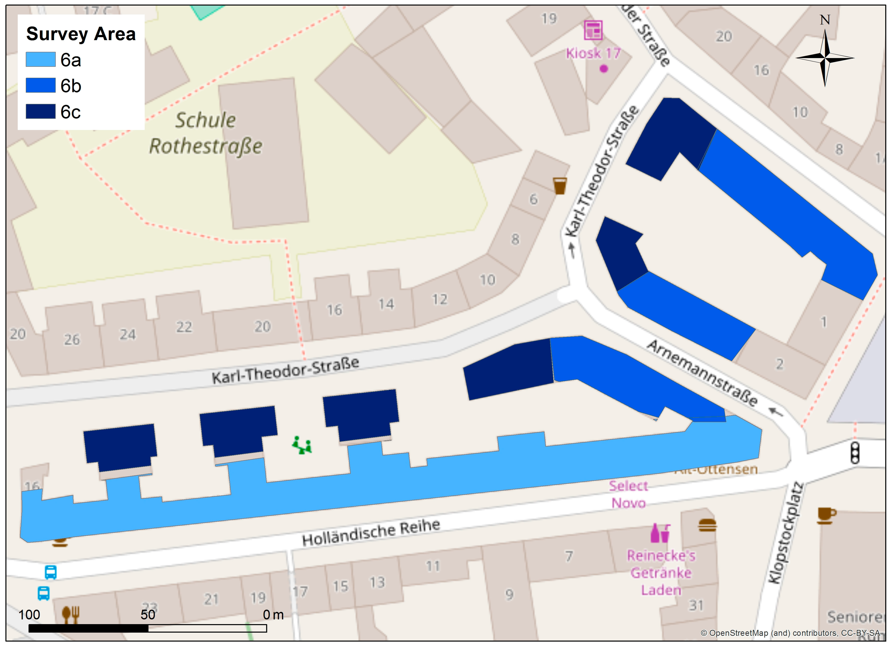
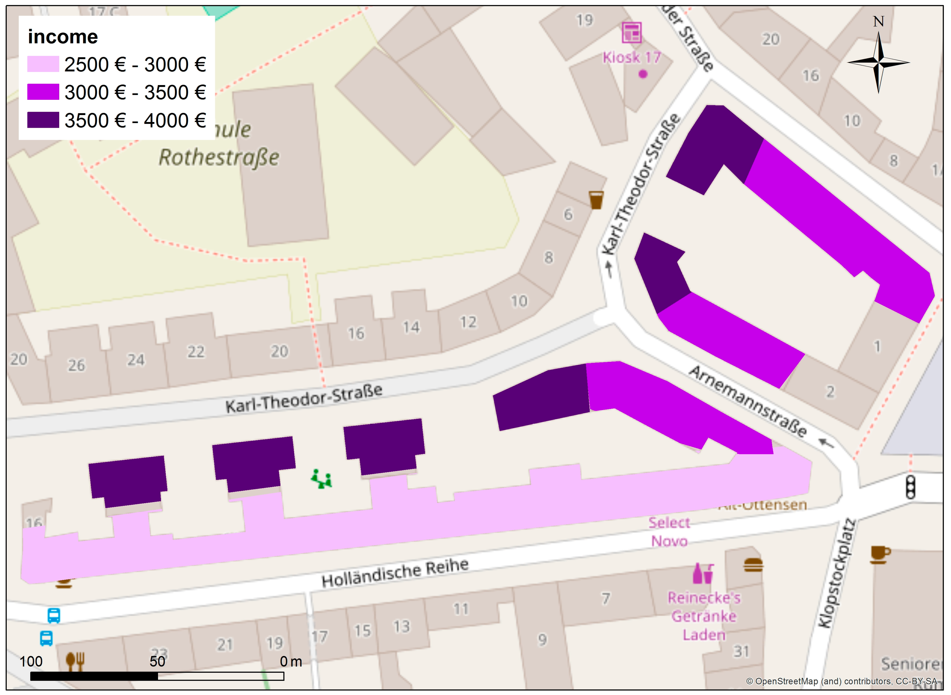
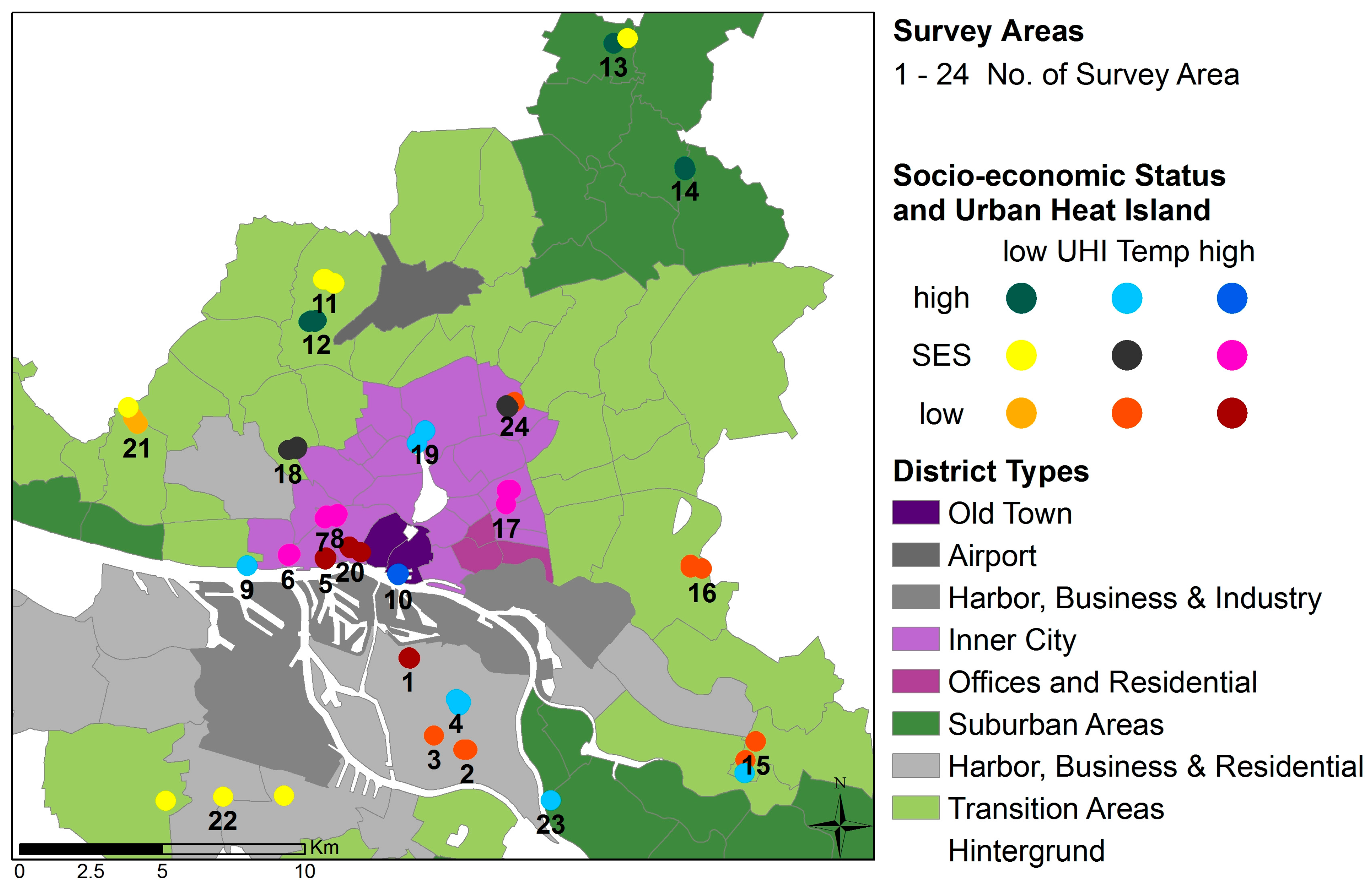
| Survey Area | District | District Type | Building Type | No. of Cases (n) |
|---|---|---|---|---|
| 1 | Wilhelmsburg | Harbor, Business & Residential | 1920s block building | 28 |
| 2 | Wilhelmsburg | Harbor, Business & Residential | 1970s large housing estate | 16 |
| 3 | Wilhelmsburg | Harbor, Business & Residential | 1950s apartment houses (rows) | 13 |
| 4 | Wilhelmsburg | Harbor, Business & Residential | 1950s row housing/town-houses/detached houses | 38 |
| 5 | Altona-Altstadt | Inner City | 1920s block building | 26 |
| 6 | Ottensen | Inner City | 1900s block building/Gap closing and re-compaction | 58 |
| 7 | Altona-Nord | Inner City | 1950s–60s apartment houses/2010s block building | 42 |
| 8 | Sternschanze | Inner City | 1900s block building | 55 |
| 9 | Othmarschen | Transition Area | 1900s apartment & detached houses | 24 |
| 10 | Hafen City | Old Town | 2010s compact mid/high rise | 53 |
| 11 | Niendorf | Transition Area | 1950s apartment houses (rows)/1970s high rise | 41 |
| 12 | Niendorf | Transition Area | 1980s/90s apartment houses/detached & townhouses | 79 |
| 13 | Duvenstedt | Suburban Area | 1900s–1990s apartment & detached houses | 30 |
| 14 | Bergstedt | Suburban Area | 1950s apartment houses (rows) | 19 |
| 15 | Neuallermöhe | Transition Area | 1980s apartment houses | 69 |
| 16 | Billstedt | Transition Area | 1960s apartment & high rise | 33 |
| 17 | Eilbek | Inner City | 1960s apartment houses (gap closing)/1990s apartment rows | 68 |
| 18 | Eimsbüttel | Inner City | 1900s/1920s block buildings/mixed gap closings | 102 |
| 19 | Winterhude | Inner City | 1900s large townhouses & mixed apartment houses | 58 |
| 20 | St. Pauli | Inner City | 1900s block building/Gap closing/2010s high rise | 60 |
| 21 | Osdorf | Transition Area | 1970s large housing estate/ detached houses | 31 |
| 22 | Moorburg/Haus-bruch/Neugraben | Transition Area/Harbor, Business & Residential | 1920s–1980s apartment & detached houses/1990s block | 37 |
| 23 | Ochsenwerder | Suburban Area | 1950s–1990s detached & apartment houses | 24 |
| 24 | Barmbek-Nord | Inner City | 1920s block building/1960s apartment houses | 77 |
| Variable | Source | Scale | No. of Cases |
|---|---|---|---|
| Lnight | Strategic noise map, city of Hamburg | dB(A) | 60 different average means (for 1024 cases) |
| Lden | Strategic noise map, city of Hamburg | dB(A) | 62 different average means (for 1057 cases) |
| Laeq | Measurements | dB(A) | 179 |
| Overall Annoyance by Noise | |||||
|---|---|---|---|---|---|
| Daytime Weekdays (NWD) | Daytime Weekends (NWE) | Nights (NNI) | Traffic Noise (NRT) | ||
| Lden | r (Spearman-Rho) | 0.23 *** | 0.19 *** | 0.23 *** | 0.42 *** |
| df | 1034 | 1018 | 1020 | 1000 | |
| Overall Annoyance by Noise | ||||
|---|---|---|---|---|
| Daytime Weekdays (NWD) | Daytime Week-Ends (NWE) | Traffic Noise (NRT) | ||
| Laeq | r (Spearman-Rho) | 0.18 * | 0.19 * | 0.60 *** |
| df | 177 | 175 | 174 | |
| Overall Annoyance by Noise | |||||
|---|---|---|---|---|---|
| Daytime Weekdays (NWD) | Daytime Weekends (NWE) | Nights (NNI) | Traffic Noise (NRT) | ||
| Age (years) | r (Spearman-ho) | 0.09 ** | 0.09 ** | 0.17 *** | 0.16 *** |
| df | 1025 | 1009 | 1011 | 991 | |
| Lden > 55–60 dB(A) | Lnight > 55–60 dB(A) | |
|---|---|---|
| Annoyance from road noise (NRT) | ➢ very much (45) = 45 years, p < 0.05 vs. somewhat (62) = 54.4 years, p < 0.05 | ➢ very much (56) = 43.1 years, p < 0.00 vs. somewhat (41) = 59 years, p < 0.00 ➢ very much (56) = 43.1 years, p < 0.00 vs. not at all (35) = 54.7 years, p < 0.00 ➢ quite (43) = 46.9, p < 0.00 vs. somewhat (41) = 59 years, p < 0.00 |
| Annoyance from noise at night (NNI) | no significant differences | ➢ quite (24) = 40.2 years, p < 0.00 vs. not at all (72) = 58.5 years, p < 0.00 ➢ somewhat (66) = 46.7 years, p < 0.00 vs. not at all (72) = 58.5 years, p < 0.00 |
© 2018 by the authors. Licensee MDPI, Basel, Switzerland. This article is an open access article distributed under the terms and conditions of the Creative Commons Attribution (CC BY) license (http://creativecommons.org/licenses/by/4.0/).
Share and Cite
Von Szombathely, M.; Albrecht, M.; Augustin, J.; Bechtel, B.; Dwinger, I.; Gaffron, P.; Krefis, A.C.; Oßenbrügge, J.; Strüver, A. Relation between Observed and Perceived Traffic Noise and Socio-Economic Status in Urban Blocks of Different Characteristics. Urban Sci. 2018, 2, 20. https://doi.org/10.3390/urbansci2010020
Von Szombathely M, Albrecht M, Augustin J, Bechtel B, Dwinger I, Gaffron P, Krefis AC, Oßenbrügge J, Strüver A. Relation between Observed and Perceived Traffic Noise and Socio-Economic Status in Urban Blocks of Different Characteristics. Urban Science. 2018; 2(1):20. https://doi.org/10.3390/urbansci2010020
Chicago/Turabian StyleVon Szombathely, Malte, Myriam Albrecht, Jobst Augustin, Benjamin Bechtel, Isabel Dwinger, Philine Gaffron, Anne Caroline Krefis, Jürgen Oßenbrügge, and Anke Strüver. 2018. "Relation between Observed and Perceived Traffic Noise and Socio-Economic Status in Urban Blocks of Different Characteristics" Urban Science 2, no. 1: 20. https://doi.org/10.3390/urbansci2010020