U.S. Metropolitan Spatial Structure Evolution: Investigating Spatial Patterns of Employment Growth from 2000 to 2010

1
Department of Landscape Architecture and Urban Planning, Texas A&M University, College Station, TX 77840, USA
2
School of Urban Planning and Design, Peking University Shenzhen Graduate School, Shenzhen 518055, China
3
Department of Geography, Texas A&M University, College Station, TX 77840, USA
4
Center for Geospatial Science, Applications and Technology (GEOSAT), Texas A&M University, College Station, TX 77840, USA
5
Zachry Department of Civil Engineering, Texas A&M University, College Station, TX 77840, USA
*
Author to whom correspondence should be addressed.
Urban Sci. 2017, 1(3), 28; https://doi.org/10.3390/urbansci1030028
Submission received: 11 July 2017
/
Revised: 4 August 2017
/
Accepted: 14 August 2017
/
Published: 22 August 2017
Abstract
:Urban spatial structure evolution, when using employment as the proxy, can be explained by the change of employment distribution. In this study, we measure the 361 US metro areas (metros) by employment shares, in five submetro sections (i.e., main-center, sub-centers, non-center clusters, non-cluster urban areas, and rural areas), and explore the spatial patterns of submetro growths. We use recognized methods to delimit urban and rural areas, identify employment centers with relative thresholds, and categorize the metros into three (i.e., small, midsize, and large) categories. Then we use descriptive statistics to determine the dynamics of employment growth in the five submetro sections. The results suggest that metros’ spatial structures and growth patterns vary greatly across different size categories. We found that (1) small metros tend to have growth in the main-center or non-cluster urban areas; (2) midsize metros may be in the critical period of forming sub-centers, which also may be an effective way to curb urban expansion into rural areas; and, (3) the five submetro growths in large metros tend to be positively associated with one another, except for the main-center.
1. Introduction
The United States (US) went through three major stages of urban spatial structure evolution. In the 1840s, the American dream indicated spreading construction to the suburbs [1]. In the 1950s, the suburban movement began as many urban residents moved to the suburbs, encouraged by affordable automobiles and government subsidies [2]. Between the late 1950s and early 1970s, many states (e.g., Kentucky, Oregon) established urban growth boundaries (UGB) to curb urban expansion [3]. According to a survey in 1991, roughly a quarter of cities used UGBs to limit urban growth areas [4]. From the American dream, suburban movement to UGBs, urban policies swung back and forth to adjust to the urban spatial structure. As a result, some policies may have positive impacts on some regions, while having negative impacts on the others.
The planning literature has identified employment centers, and the growth within and outside of them. In other words, the spatial structure of metro areas (interchangeably “metros” or “cities” in this paper) may evolve towards concentration or dispersion (including decentralization). Earlier studies [5,6,7] have disagreed on whether cities are edged or edgeless. The former suggests that a re-concentration process occurs at a city’s edge during expansion, while the latter suggests that urban development is largely scattered—cities are edgeless. More recent studies [8,9,10,11,12,13,14] found both concentration and dispersion in different metros, and also in different employment sub-centers within a single metro. These are mainly case studies that cannot demonstrate their theories’ applicability to a larger sample of metros.
Given the literature review, two big questions arise. The first question is in regards to the origin and destination of the employment concentration and dispersion (including decentralization). Where does the employment move to when it spreads from the Central Business District (CBD)? Does it go to sub-centers, non-center areas, or does it move outside of the metro? The second question involves employment clusters that are smaller than an employment center (typically defined as a minimum size of 10,000 workers), but that display certain agglomerative power. These areas have largely been neglected in empirical studies. Is it really safe to say that agglomeration economies at the submetro level are no longer important? Or, maybe agglomeration economies are presenting themselves in a new form? In fact, a few studies [15,16,17,18,19,20,21] point out the complexity of the metropolitan spatial structures. They describe the structural complexity as being “beyond polycentricity” [19], a network of “trading places” [20], and “complex variation in density” [21]. After all, the formation of an employment center is a gradual process; it inevitably generates employment clusters of varying sizes. A metropolitan spatial structure is more than a dual system of employment centers and non-center areas.
Studies on employment centers implicitly include four submetro sections: the CBD, sub-centers, urban areas, and rural areas. The CBDs are easy to define for small-sized (e.g., case-study based, descriptive) studies. It is also common to define the largest employment center as the CBD [11], but we can cautiously use the term “main-center” in the case that some metro areas’ CBDs are smaller than their sub-centers. There are also recognized methods to delimit urban and rural areas [11,22], and to identify employment centers [23,24,25,26]. However, no study gives equal attention to all of these submetro sections; instead, most studies only analyze employment dynamics within and outside of the employment centers.
This paper investigates the dynamics of employment growth in five submetro sections that include four implicit ones (the main-center, sub-centers, non-cluster urban areas, and rural areas) in the literature and the non-center clusters. We use the entire country as the study area, and the longest time frame available. Next, we divide the metros into three size categories, since metros of different sizes may behave differently, e.g., the formation of sub-centers requires a population size threshold [24,27]. Then we explore the employment shares in 2000 and 2010, as well as the correlations of employment growth in these five submetro sections. In this study, we make two major assumptions. First, we assume that the growth of the metros is independent, e.g., two metros’ main-centers are not correlated with one another. Second, we assume that the metros are mature economic units that are highly diverse in industrial composition. Although different employment clusters in a metro may change in different directions (e.g., decline, remain) [7], in this study we look at the average effect of each submetro section, e.g., the sum of all sub-centers as a submetro section.
The significance of this study is twofold. First, the dynamics of employment growth in five submetro sections can provide policymakers with more accurate knowledge for proactive planning. Especially, we add the section of non-center clusters, which represent the gradual process of forming a sub-center; these clusters may also play a significant role in capturing agglomeration economies. Second, most studies on US metropolitan structure focus on the major metros (e.g., Los Angeles, Chicago); the repeated emphasis on the same cities results in biased understanding regarding the US metro structure as a whole. Additionally, those case studies provide little insight for small and midsize metros’ growth patterns. Our detailed analysis of all US metros paints a more complete picture of the US metro structure, which may serve as a benchmark for national and regional policy reference.
2. Data and Method
2.1. Data
We use shape files from the Topologically Integrated Geographic Encoding and Referencing (TIGER), and employment data are from the Census Transportation Planning Products (CTPP). TIGER provides shape files that define the metros’ boundaries and census tracts within the metros. The metros in this study come from the Metros in the Core Based Statistical Area (MCBSA) system. In the US (and Puerto Rico), there are 370 metros in the Census 2000 TIGER shape file. However, we exclude the eight Puerto Rico metros because no employment data were available. Within the 362 MCBSAs, Bristol, VA became a part of Kingsport-Bristol-Bristol, TN-VA. Therefore, we examine 361 metros. As the population grows, the Census alters the boundaries of census tracts. As we have observed, this alteration is negligible from year 2000 to 2010. Most (more than 99.9 percent) census tracts remained the same.
CTPP provides employment data summarized at the census tract level. We join the 2000 and 2010 CTPP employment data to the year 2000 TIGER shape files to obtain employment data for each census tract. The year 2000 and year 2010 employment data were collected by the US Census Bureau.
2.2. Method
2.2.1. Defining Five Submetro Sections
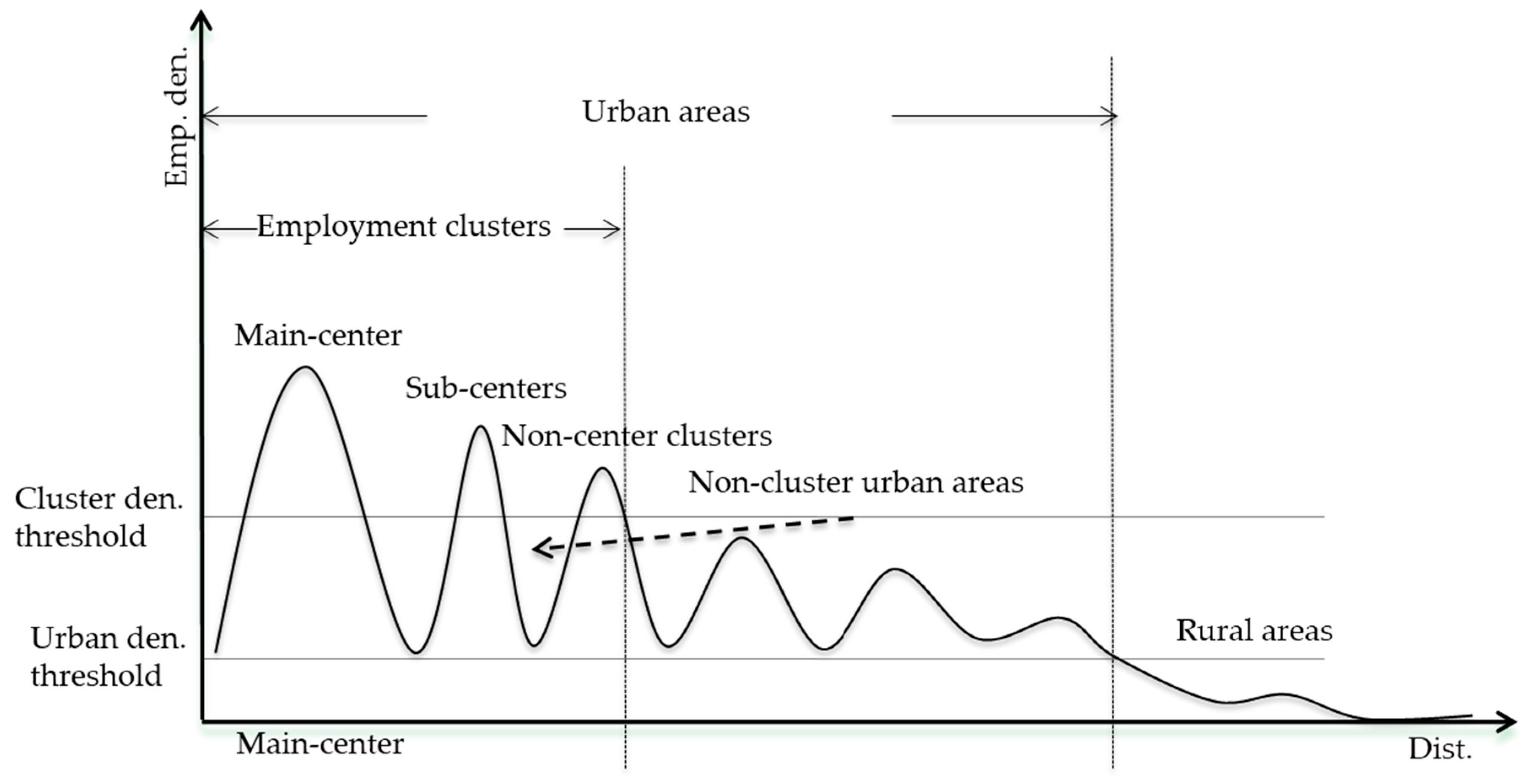
To capture the inner structural characteristics, we separate a metro into five submetro sections: the main-center, sub-centers, non-center clusters, non-cluster urban areas, and rural areas (see Figure 1). The main-center is defined as the largest employment center in a metro. Except for the main-center, all other submetro sections are aggregate configurations. The section of sub-centers is the sum of all employment centers except for the main-center. Note that we do not attempt to count each metro’s employment centers for this countrywide study. For one thing, the exact number is difficult to determine because two or more centers may be connected; for another, slightly different total employment threshold (that is usually arbitrary and based on local knowledge) may result in a different number of employment centers. Similarly, the section of non-center clusters is the sum of all employment clusters smaller than employment centers. The section of non-cluster urban areas is the sum of all urban areas excluding the employment clusters (i.e., the main-center, sub-centers, and non-center clusters). The section of rural areas is the remaining areas in a metro, excluding the urban areas. The sum of employment in the five submetro sections equals the metro’s total employment.
To enable comparisons among different submetro sections, we separate a metro by an urban density threshold, a cluster density threshold, and a center size threshold; see Table 1. The urban density threshold delimits urban and rural areas. The cluster density threshold delimits employment clusters, and non-cluster urban areas. The center size threshold delimits the employment centers, and non-center clusters. In other words, the main-center meets all three of the criteria (and having the largest employment center), and the rural areas meet no criterion, and so on. The following Section 2.2.2 and Section 2.2.3 will demonstrate calculation of the three thresholds (i.e., an urban density threshold, a cluster density threshold, and a center size threshold).
2.2.2. Delimiting Urban and Rural Areas
To ensure homogeneity of data units (i.e., census tracts) in a metro, we delimit the urban and the rural areas, because spatial indices are “sensitive to the presence of large, unpopulated census tracts in outlying areas due to the well-known mismatch of administrative boundaries and functional areas” [11] (p. 485). There are absolute and relative threshold methods to delimit the urban and rural areas. The absolute threshold method adopts a universal cutoff for all metros, such as 1000 persons per square mile as defined by the Census. This definition may inappropriately exclude large areas of developed land [3]. Conversely, the relative threshold method applies a cutoff percentage to a metro’s total population. The cutoff percentage may be 98 percent [22], or 95 percent [11].
We choose the relative [11,22] over the absolute methods [3,23], considering the large variations of employment densities across US metros. We also choose to use employment instead of population, because employment is better than population (based on primary residences) in capturing urban activity. For example, activity centers such as the Central Business Districts often have few residents.
After testing three percentages, we determine 98 percent as the most reasonable threshold to delimit urban and rural areas. Because population is generally larger than employment (especially in rural areas), we initially try to define urban areas as having 99 percent of employment. However, the resulting polygons include large swathes of mountainous terrain that are not urban. Then we try 95 percent. The resulting polygons, however, exclude many near urban center tracts that are urban. Finally, defining urban areas as having 98 percent of employment produces a more reasonable result than using the 99 percent and the 95 percent choices.
We separate the census tract (polygons), with the lowest year 2000 employment density from a metro one by one until the total employment is as close to (but not less than) 98 percent of the year 2000 total employment. The remaining census tracts within the MCBSA are the urban tracts. The rest census tract polygons are rural tracts whose employment amounts to roughly 2 percent of the metro’s total employment.
2.2.3. Identifying Employment Clusters
Similar to delimiting urban and rural areas, identifying clusters involves either absolute or relative threshold criteria. One method adopts an absolute density (e.g., 10 workers/acre) and a total employment threshold (e.g., 10,000 workers) [23]. A second method adopts a regression model (e.g., locally weighted regression) on distance from the Central Business District, to identify secondary density peaks and uses a geographic window to ensure the secondary peaks have statistically significantly higher density than their surroundings [24]. The third method adopts a percentile threshold to identify a metro’s densest areas as potential employment centers, and then applies a total employment threshold (e.g., 10,000 workers) to remove small-size employment clusters [11,23,25].
We adopt the third method because it meets the following criteria: (1) it is capable of capturing each metro’s structural feature; (2) it is easy to use for a large sample; and, (3) it uses a consistent density threshold throughout a metro. Conversely, the first and second methods have the following drawbacks. The first method can only capture the spatial features of high-density metros. This method is not applicable for large sample size studies. The second method results in inconsistent density thresholds within a metro, and complicates the comparative analysis on submetro sections. Furthermore, the second method is also arbitrary in choosing the “significance level, geographic window size, and weight of distance” [26] (p. 27).
Note that by using the third method, the calculated density thresholds may not always qualify in accordance with our traditional understanding of sub-centers. For this national study, the density threshold is determined by each metro’s density distribution. Some metros’ density threshold may be too low or too high, but these thresholds will not affect the effectiveness of this study. For example, a threshold of 2 workers/acre may not qualify to identify a mature employment center. However, this extremely low-density threshold is acceptable in this study, for it still captures the relatively dense areas in a metro; and these areas denote where the future sub-centers will be. Additionally, what we aim to examine is the growth in these areas. But we may not interpret some of the sub-center areas as matured sub-centers yet.
To apply the third method, we identify clusters by selecting high-density urban tracts and merging the neighboring tracts into a zone. High-density urban tracts have a density above the metro’s cluster density threshold. Each metro’s cluster density threshold equals two standard deviations above the metro’s mean employment density in urban areas. In equation (1), the probability (P) is a census tract’s area, proportional to a metro’s total urban land area, P = . The mean density (U) is a metro’s total employment in the urban land area divided by the urban land area, U = . A metro’s total urban land area is the sum of all census tract areas in the urban areas, = . For metro , we have:
where,
—Metro ’s cluster density threshold; = 1, 2, 3, …, 361;
—Urban tract ’s area in metro j; = 1, 2, 3, …, ( = metro ’s total number of urban tracts);
—Urban tract ’s density in metro j.
To separate the employment centers and non-center clusters, we define the center size threshold at 10,000 workers (the same as previous studies). In other words, we define employment clusters with over 10,000 workers as employment centers, otherwise as non-center clusters. The arbitrary size threshold of 10,000 workers is broadly used in existing literature [11,13,23]. The theoretical support for this arbitrary size threshold can be traced back to the urban size ratchet concept [28]. We assume that a size of 10,000 workers is large enough to sustain an area’s local market. Empirically, we choose this center size threshold to enable comparison with previous studies, and furthermore, the debate on reasonable local market (city) size has little consensus in existing literature.
3. Results
3.1. A Metro’s Five Submetro Sections
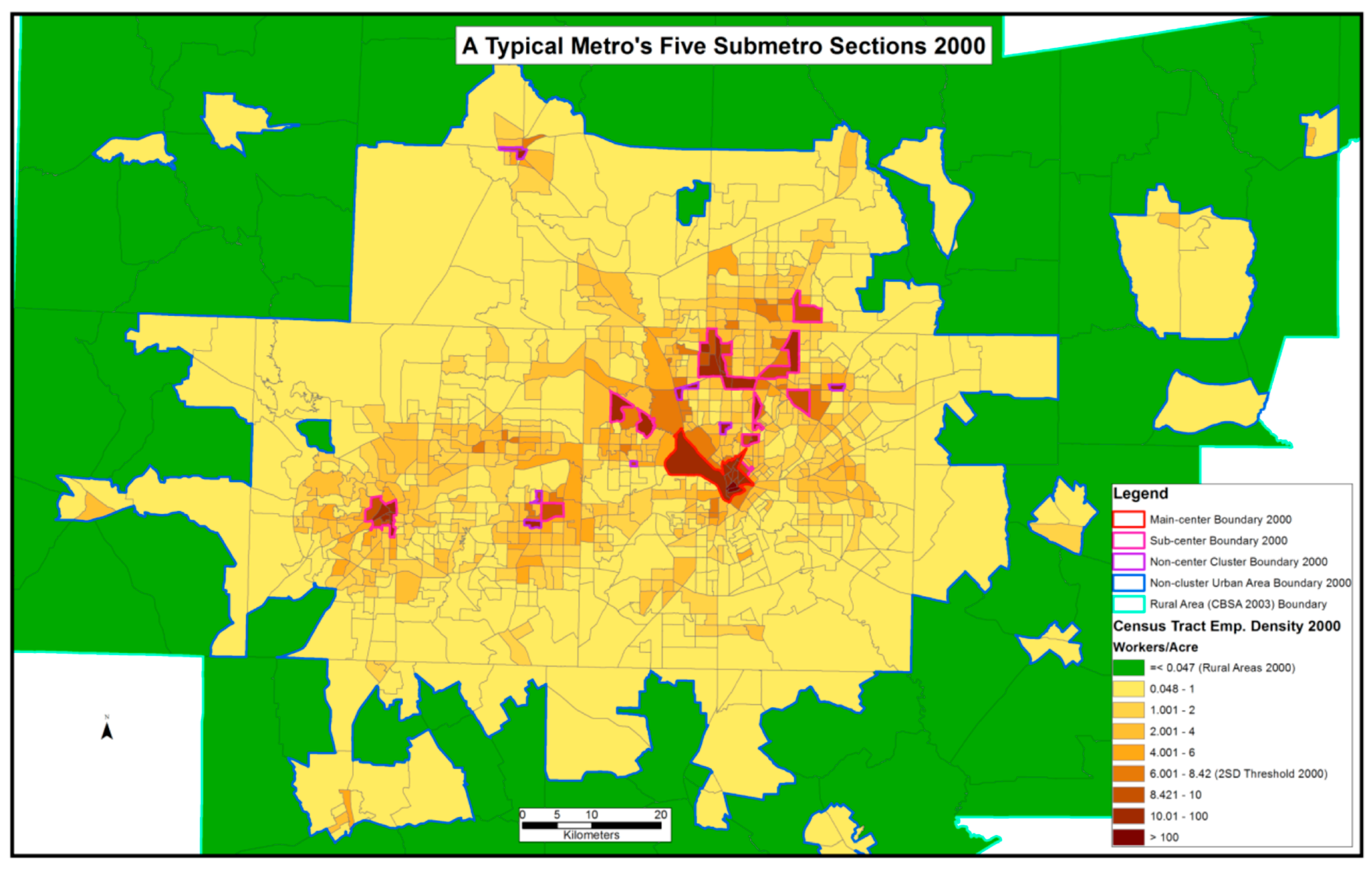
Using the metro “Dallas–Fort Worth–Arlington, TX” as an example, we interpret the metro’s five submetro sections. We use the year 2000 data to calculate the two density thresholds (i.e., urban density threshold, and cluster density threshold), and apply them to year 2000 and 2010 structural measurements. As Figure 2 and Figure 3 show, the urban density threshold is 0.047 workers/acre. Areas with a density below 0.047 workers/acre are the rural areas (green areas) on both year 2000 and 2010 maps. Note that on the year 2010 map, we use the same urban areas boundary (blue line) as on the year 2000 map, in order to observe the urban developments that happened in the former rural areas. The cluster density threshold is 8.42 workers/acre. Areas with a density above the cluster density threshold are employment clusters that can be the main-center, sub-centers, or non-center clusters, depending on their cluster sizes. The largest employment cluster, also employment center, is the main-center with a red boundary. The sub-centers have pink boundaries, and the non-center clusters have purple boundaries.
3.2. Spatial Structure Charateristics
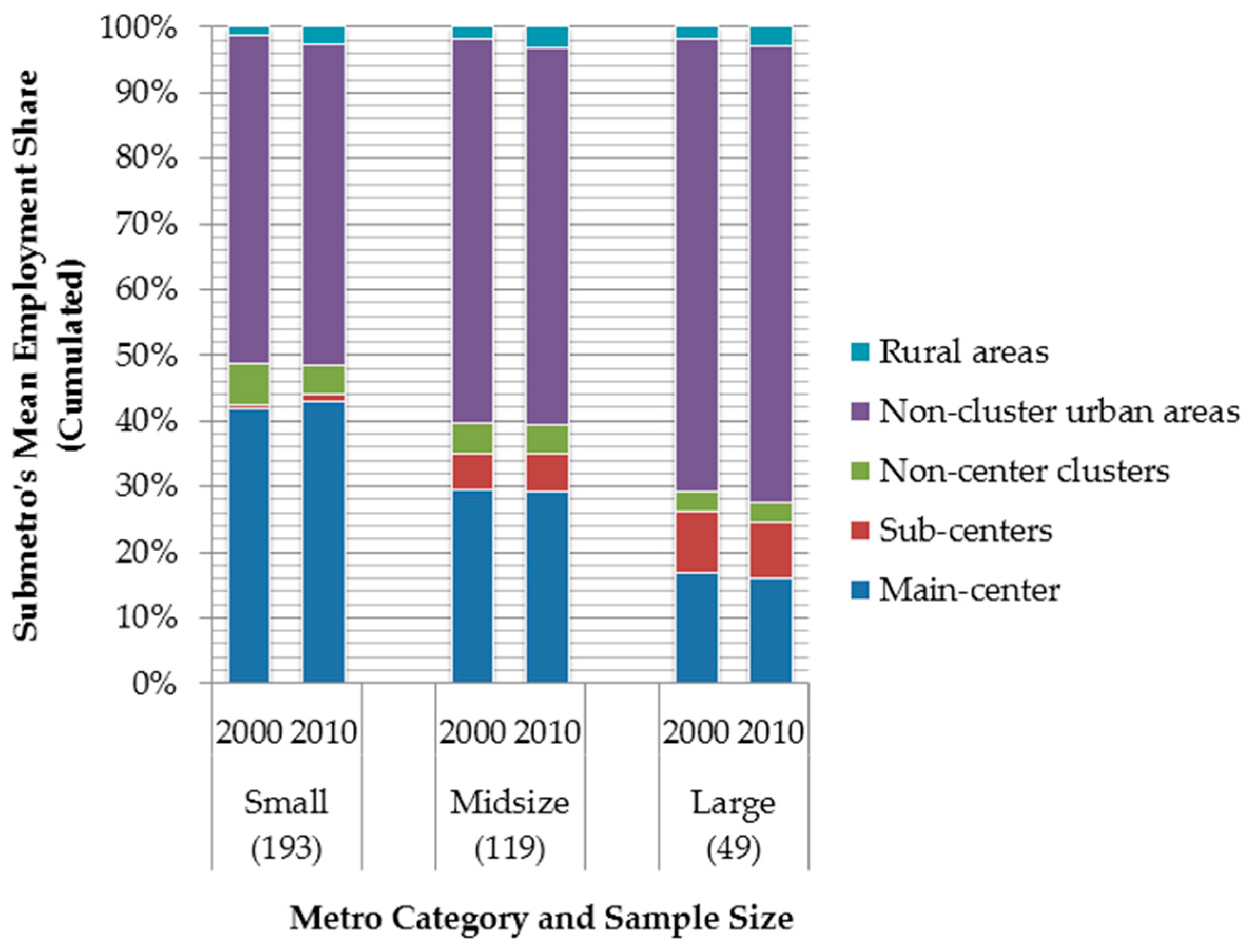
We divide metros into three categories according to population in 2000: large metros’ population ≥ one million; a quarter million ≤ midsize metros’ population < one million; and, small metros’ population < a quarter million. There are 49 large, 119 midsize, and 193 small metros. Note that this is the only time that we use population in our analysis. Although employment is more appropriate to represent agglomeration economies (e.g., agglomeration of firms), population is more traditionally used for simple categorization based on size. We select the thresholds of one million and a quarter million based on academic and practical examples. Studies commonly select the largest 50 metros to represent the characteristics of the entire urban US [21,29]. Coincidently, the threshold of one million results in the largest 49 metros, which makes the category of large metros comparable with other studies. Additionally, the National Center for Health Statistics (NCHS) data systems, used for studying the associations between residence’s urbanization level and health, also adopt the thresholds of one million and a quarter million to categorize the US metros into three categories [30]. Although alternative thresholds may be used, we consider these two as the most reasonable ones for a national study. Besides, one may divide the metros into more categories for more refined results, in light of the methods used in this study.
Figure 4 shows the mean employment shares in each metro category (i.e., large, midsize, small) in 2000 and 2010. We found that larger metros tend to have lower mean employment shares in the main-center, but higher mean employment shares in the sub-centers and non-cluster urban areas. However, comparing the mean initial and ending spatial structures gives little insight to the metros’ evolution process. In other words, the metros’ mean employment shares largely remain the same from 2000 to 2010. Two questions arise. Is this because the submetro growth shares are proportionate to their initial employment shares? Is this because submetro growths of different metros cancel out, resulting in a nearly zero effect on average? To answer the first question, we investigate the distribution of metro growth among the five submetro sections. To answer the second question, we build correlation matrices to examine how each metro’s submetro growth deviates from that of other metros.
3.3. The Distribution of Employment Growth
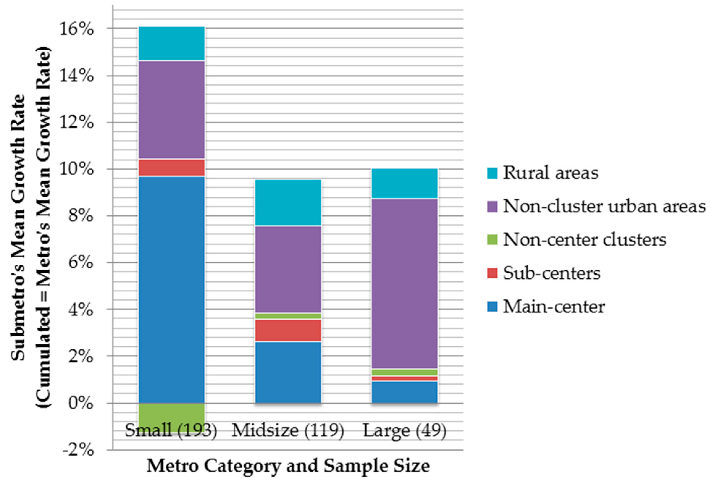
In this section, we examine whether the submetro growth shares are proportionate to their initial employment shares. We divide each metro’s submetro growth (amount) by the metro’s total employment in 2000, and the result is the submetro growth share. The sum of the five submetro growth shares equals the metro’s growth rate. We report the mean values of the five submetro growth shares in each metro category in Figure 5.
As Figure 5 shows, the submetro growth shares in each metro category are not proportionate to their initial employment shares (as indicated in Figure 4). For example, small metros’ mean growth share in the main-center is greater than the sum of the other four growth shares, which is different from their initial distribution of employment shares. Additionally, small metros have negative mean growth shares in the non-center cluster areas; this may be because employment in non-center cluster areas agglomerates into employment centers, or disperses into non-cluster urban areas or even into rural areas. Midsize metros’ mean growth share in the sub-centers is much greater than that in the non-center clusters, while initially the employment shares in the two submetro sections are nearly the same. In fact, midsize metros’ mean growth share in the sub-centers is the largest among the three categories. For large metros, the mean growth shares in the non-cluster urban areas and rural areas greatly exceed their initial employment shares, which indicates a low-density growth pattern because those two submetro sections are the lowest density areas in a metro. Meanwhile, the mean growth shares in the sub-centers and non-center clusters are extremely small, indicating that metros have largely completed sub-centering before entering into the large metro category.
3.4. The Correlations of Submetro Growth
In this section, we examine how each metro’s submetro growth deviates from that of other metros by creating three correlation matrices. A correlation coefficient suggests the strength of the relationship between two sets of variables. For this study, we do not need the direction of the relationship. Note that the following three tables show the correlations of net growth (rather than growth rate) in the five submetro sections.
Table 2 shows that: (1) small metros’ main-centers compete with the other four submetro sections: sub-centers, non-center clusters, non-cluster urban areas, and rural areas, in decreasing order of likelihood; (2) metro growth tends to happen in the main-centers and non-cluster urban areas; and, (3) employment in non-center clusters tends to disperse into non-cluster urban areas, given non-cluster urban areas’ positive association with metro growth (0.40), and negative association with the non-center clusters (−0.14).
Table 3 shows that midsize metros’ sub-centers agglomerate employment from the non-center clusters (−0.28) and rural areas (−0.22). Accordingly, the non-center clusters and rural areas are the only submetro sections that do not significantly associate with metro growth. The negative correlation between the sub-centers and rural areas suggests that forming sub-centers should be an effective method to curb urban expansion (to rural areas).
Table 4 shows that the large metros’ growth is largely characterized by low-density growth, with all the submetro growths positively associated with one another, except for the competition between the main-center and the sub-centers. The low-density growth is indicated by the positive correlation of metro growth with growths in non-cluster urban areas (0.89) and rural areas (0.66). Besides those two, the other three coefficients in the bottom row are all rounded to be 0.41 (main-center > non-cluster urban areas > sub-centers). The only moderately strong negative correlation, however, is between the main-center and sub-centers (−0.22). This indicates that the main-center and sub-centers may compete with one another in some metros. Finally, the absolute values of coefficients are relatively large in general, indicating large metros’ growth pattern is more stable than that of small and midsize metros.
4. Discussion and Conclusions
This paper investigated US metros’ spatial structures and evolution patterns. We use employment shares in five submetro sections to denote a metro’s spatial structure and use submetro growth patterns to describe the metro’s evolution process. The measurement methods are adopted from literature with minor modifications. We aim to make the methods easy to understand and applicable to the entire country. This study takes a closer look into the metropolitan spatial structures for all 361 metros. Policymakers can clearly see which stage their metro is currently at, and which stage it is heading to, as well as identifying similar metros. Additionally, other countries may use the same methods to conduct their own countrywide study.
We found that metros’ evolution patterns vary greatly across the three size categories. First, small metros’ main-centers agglomerate employment from the other four submetro sections: sub-centers, non-center clusters, non-cluster urban areas, and rural areas, in decreasing the order of likelihood. Non-center clusters tend to disperse into non-cluster urban areas. Therefore, for metros with a population of less than a quarter million, policymakers should focus the resources on creating jobs in the main-centers.
Second, midsize metros seem to be in the critical period to form sub-centers and reduce urban expansion (to rural areas). Midsize metros’ sub-centers have the largest mean growth share among the three categories, and not only compete with the non-center clusters but also the rural areas. Additionally, unlike large metros, midsize metros have a relatively large room for urban development. Therefore, for metros with a population of over a quarter but less than a million, policymakers should provide more convenience for sub-center development.
Third, large metros’ evolution patterns are of high regularity: Growths in the five submetro sections positively associate with one another, except for the main-center (that competes with the sub-centers). Additionally, large metros are much more likely to have growth in the low-density areas (i.e., non-cluster urban areas and rural areas) than the high-density areas. In fact, the growths in the sub-centers and non-center clusters are extremely small, indicating that the metros have already completed sub-centering before entering into the large metro category. This further confirms the importance of laying out a proactive plan at the midsize metro stage. After a metro’s population exceeds one million, large-scale changes to its spatial structure become difficult, but policymakers can still put efforts in increasing the development density and renewing the main-center.
Author Contributions
Xiaoyan Huang conceived the idea and wrote the paper. Jiawen Yang reshaped the paper with clear focus. Burak Güneralp instructed academic writing in detail. Mark Burris inspected the data, formulas and technical accuracy, as well the content’s logic flow and conciseness.
Conflicts of Interest
The authors declare no conflict of interest.
References
- O’Sullivan, J.L. The great nation of futurity. U.S. Democr. Rev. 1839, 6, 426–430. [Google Scholar]
- Duany, A.; Plater-Zyberk, E.; Speck, J. Suburban Nation: The Rise of Sprawl and the Decline of the American Dream; Farrar, Straus and Giroux: New York, NY, USA, 2001. [Google Scholar]
- Lopez, R.; Hynes, H.P. Sprawl in the 1990s measurement, distribution, and trends. Urban Aff. Rev. 2003, 38, 325–355. [Google Scholar] [CrossRef] [PubMed]
- O’sullivan, A. Urban Economics; McGraw-Hill/Irwin: New York, NY, USA, 2007. [Google Scholar]
- Garreau, J. Edge City: Life on the New Frontier; Doubleday: New York, NY, USA, 1991. [Google Scholar]
- Krugman, P.R.; Venables, A.J. Globalization and inequality of nations. Q. J. Econ. 1995, 110, 857–880. [Google Scholar] [CrossRef]
- Cervero, R.; Wu, K.L. Polycentrism, commuting, and residential location in the San Francisco Bay area. Environ. Plan. A 1997, 29, 865–886. [Google Scholar] [CrossRef] [PubMed]
- Lang, R.E. Edgeless Cities: Exploring the Elusive Metropolis; Brookings Institution Press: Washington, DC, USA, 2003. [Google Scholar]
- Giuliano, G.; Small, K.A. The determinants of growth of employment subcenters. J. Transp. Geogr. 1999, 7, 189–201. [Google Scholar] [CrossRef]
- McMillen, D.P.; Lester, T.W. Evolving subcenters: Employment and population densities in Chicago, 1970–2020. J. Hous. Econ. 2003, 12, 60–81. [Google Scholar] [CrossRef]
- Lee, B. Edge or edgeless cities? Urban spatial structure in U.S. metropolitan areas, 1980 to 2000. J. Reg. Sci. 2007, 47, 479–515. [Google Scholar] [CrossRef]
- Giuliano, G.; Agarwal, A.; Redfearn, C.; Traveled, V.M. Metropolitan Spatial Trends in Employment and Housing. Available online: http://onlinepubs.trb.org/Onlinepubs/sr/sr298giuliano.pdf (accessed on 14 August 2017).
- Redfearn, C.L. Persistence in urban form: The long-run durability of employment centers in metros. Reg. Sci. Urban Econ. 2009, 39, 224–232. [Google Scholar] [CrossRef]
- Cervero, R.; Komada, Y.; Krueger, A. Suburban Transformations: From Employment Centers to Mixed-Use Activity Centers. Available online: http://escholarship.org/uc/item/9h8387sz (accessed on 1 August 2017).
- Anas, A.; Arnott, R.; Small, K.A. Urban spatial structure. J. Econ. Lit. 1998, 36, 1426–1464. [Google Scholar]
- Batty, M. Building a science of cities. Cities 2012, 29, S9–S16. [Google Scholar] [CrossRef]
- Batty, M. The size, scale, and shape of cities. Science 2008, 319, 769–771. [Google Scholar] [CrossRef] [PubMed]
- Bettencourt, L.M.A. The origins of scaling in cities. Science 2013, 340, 1438–1441. [Google Scholar] [CrossRef] [PubMed]
- Gordon, P.; Richardson, H.W. Beyond polycentricity: The dispersed metropolis, Los Angeles, 1970–1990. J. Am. Plan. Assoc. 1996, 62, 289–295. [Google Scholar] [CrossRef]
- Bogart, W.T. Don’t Call It Sprawl: Metropolitan Structure in the Twenty-First Century; Cambridge University Press: New York, NY, USA, 2006. [Google Scholar]
- Yang, J.; French, S.; Holt, J.; Zhang, X. Measuring the Structure of U.S. Metropolitan Areas, 1970–2000: Spatial Statistical Metrics and an Application to Commuting Behavior. J. Am. Plan. Assoc. 2012, 78, 197–209. [Google Scholar] [CrossRef]
- Wheaton, W.C. Commuting, congestion, and employment dispersal in cities with mixed land use. J. Urban Econ. 2004, 55, 417–438. [Google Scholar] [CrossRef]
- Giuliano, G.; Small, K.A. Subcenters in the Los Angeles region. Reg. Sci. Urban Econ. 1991, 21, 163–182. [Google Scholar] [CrossRef]
- McMillen, D.P.; Smith, S.C. The number of subcenters in large urban areas. J. Urban Econ. 2003, 53, 321–338. [Google Scholar] [CrossRef]
- Pan, Q.; Ma, L. Employment subcenter identification: A GIS-based method. Tex. South. Univ. Sci. Urban Econ. 2006, 21, 63–82. [Google Scholar]
- Matsuo, M. Metropolitan Form, Transportation, And Labor Accessibility—Empirical Evidence from Four US Metropolitan Areas. Ph.D. Thesis, Harvard University, Cambridge, MA, USA, 2008. [Google Scholar]
- Fujita, M.; Ogawa, H. Multiple Equilibria and Structural Transition of Non-Monocentric Urban Configurations. Reg. Sci. Urban Econ. 1982, 12, 161–196. [Google Scholar] [CrossRef]
- Thompson, W.R. A Preface to Urban Economics; Resources for the Future: Washington, DC, USA, 1965; Volume 43. [Google Scholar]
- Lee, B.; Gordon, P. Urban spatial structure and economic growth in us metropolitan areas. In Proceedings of the 46th Annual Meeting of the Western Regional Science Association, Newport Beach, CA, USA, 21–24 February 2007. [Google Scholar]
- U.S. Department of Health & Human Services (National Center for Health Statistics). NCHS Urban-Rural Classification Scheme for Counties. Available online: https://www.cdc.gov/nchs/data_access/urban_rural.htm (accessed on 7 August 2017).
Figure 1.
The definitions of a metro’s spatial constituents. (Note that the urban areas between the employment clusters are also non-cluster urban areas.)
Figure 1.
The definitions of a metro’s spatial constituents. (Note that the urban areas between the employment clusters are also non-cluster urban areas.)

Figure 2.
A typical metro’s (Dallas–Fort Worth–Arlington, TX) five submetro sections in 2000.

Figure 3.
A typical metro’s (Dallas–Fort Worth–Arlington, TX) five submetro sections in 2010.
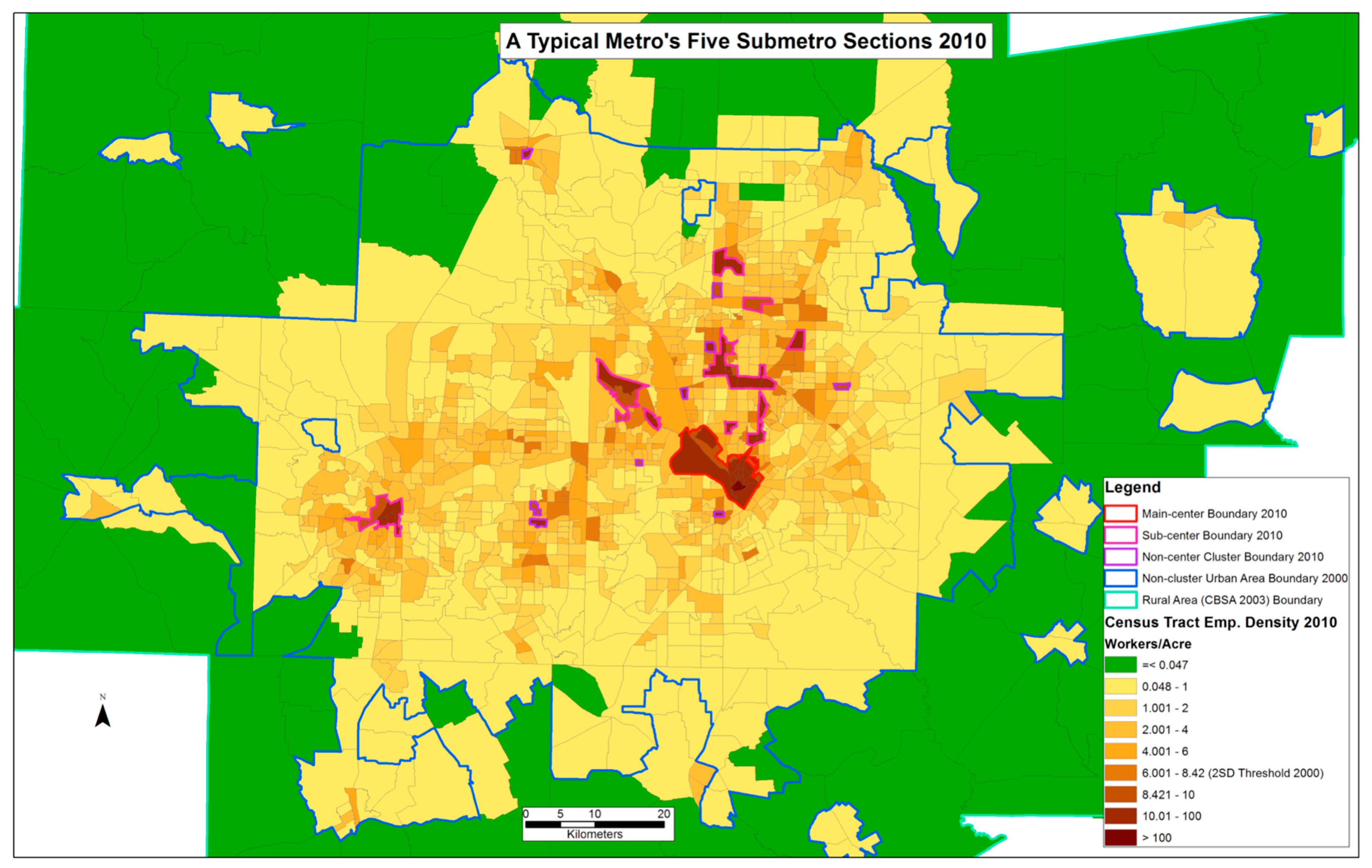
Figure 4.
Three metro categories’ mean employment shares in five submetro sections in 2000 and 2010.
Figure 4.
Three metro categories’ mean employment shares in five submetro sections in 2000 and 2010.

Figure 5.
The mean growth shares of five submetro sections in three metro categories.


Table 1.
The three thresholds to separate a metro into five submetro sections.
| Thresholds | Main-Center | Sub-Centers | Non-Center Clusters | Non-Cluster Urban Areas | Rural Areas |
|---|---|---|---|---|---|
| Urban Density | √ | √ | √ | √ | |
| Cluster Density | √ | √ | √ | ||
| Center Size | √√ | √ |
Table 2.
Correlation matrix for growth in five submetro sections for small metros.
| Section of Growth | Section No. | 1 | 2 | 3 | 4 | 5 | 6 |
|---|---|---|---|---|---|---|---|
| Main-center | 1 | 1 | |||||
| Sub-centers | 2 | −0.25 * | 1 | ||||
| Non-center clusters | 3 | −0.22 * | −0.03 | 1 | |||
| Non-cluster urban areas | 4 | −0.17 * | −0.02 | −0.14 * | 1 | ||
| Rural areas | 5 | −0.14 | 0.04 | 0 | 0.02 | 1 | |
| Metro | 6 | 0.67 * | 0.10 | 0.08 | 0.40 * | 0.12 | 1 |
Note: The number of observations is 193; and the star superscript * suggests a statistically significant correlation at the 0.05 level.
Table 3.
Correlation matrix for growth in five submetro sections for midsize metros.
| Section of Growth | Section No. | 1 | 2 | 3 | 4 | 5 | 6 |
|---|---|---|---|---|---|---|---|
| Main-center | 1 | 1 | |||||
| Sub-centers | 2 | 0 | 1 | ||||
| Non-center clusters | 3 | −0.1 | −0.28 * | 1 | |||
| Non-cluster urban areas | 4 | −0.1 | −0.14 | −0.04 | 1 | ||
| Rural areas | 5 | −0.14 | −0.22 * | −0.15 | 0.16 | 1 | |
| Metro | 6 | 0.54 * | 0.27 * | 0.04 | 0.59 * | 0.18 | 1 |
Note: The number of observations is 119; and the star superscript * suggests a statistically significant correlation at the 0.05 level.
Table 4.
Correlation matrix for growth in five submetro sections for large metros.
| Section of Growth | Section No. | 1 | 2 | 3 | 4 | 5 | 6 |
|---|---|---|---|---|---|---|---|
| Main-center | 1 | 1 | |||||
| Sub-centers | 2 | −0.22 | 1 | ||||
| Non-center clusters | 3 | 0.04 | 0.29 * | 1 | |||
| Non-cluster urban areas | 4 | 0.16 | 0.24 | 0.27 | 1 | ||
| Rural areas | 5 | 0.19 | −0.02 | 0.27 | 0.54 * | 1 | |
| Metro | 6 | 0.41 * | 0.41 * | 0.41 * | 0.89 * | 0.66 * | 1 |
Note: The number of observations is 49; and the star superscript * suggests a statistically significant correlation at the 0.05 level.
© 2017 by the authors. Licensee MDPI, Basel, Switzerland. This article is an open access article distributed under the terms and conditions of the Creative Commons Attribution (CC BY) license (http://creativecommons.org/licenses/by/4.0/).
Share and Cite
MDPI and ACS Style
Huang, X.; Yang, J.; Güneralp, B.; Burris, M. U.S. Metropolitan Spatial Structure Evolution: Investigating Spatial Patterns of Employment Growth from 2000 to 2010. Urban Sci. 2017, 1, 28. https://doi.org/10.3390/urbansci1030028
AMA Style
Huang X, Yang J, Güneralp B, Burris M. U.S. Metropolitan Spatial Structure Evolution: Investigating Spatial Patterns of Employment Growth from 2000 to 2010. Urban Science. 2017; 1(3):28. https://doi.org/10.3390/urbansci1030028
Chicago/Turabian StyleHuang, Xiaoyan, Jiawen Yang, Burak Güneralp, and Mark Burris. 2017. "U.S. Metropolitan Spatial Structure Evolution: Investigating Spatial Patterns of Employment Growth from 2000 to 2010" Urban Science 1, no. 3: 28. https://doi.org/10.3390/urbansci1030028