Finite Element Modelling and Retained Life Estimation of Corroded Pipelines in Consideration of Burst Pressures—A Fractural Mechanics Approach


Engineering Product Development Pillar, Singapore University of Technology and Design, 8 Somapah Road, Singapore 487372, Singapore
Infrastructures 2017, 2(4), 15; https://doi.org/10.3390/infrastructures2040015
Submission received: 22 August 2017
/
Revised: 10 October 2017
/
Accepted: 13 October 2017
/
Published: 15 October 2017
Abstract
:This study used Finite Element Modelling (FEM) to determine the relationship between the burst pressure (Pb) of internally, circumferentially corroded pipelines, with the corrosion defect depth (d), pipe wall thickness (t) and the pipe diameter (D). After modelling X46 and X52 grades of pipes, the Pb estimated was compared with those determined experimentally and with industry standard models—ASME B31G (modified), RSTRENG, DNV F101, SHELL92 and FITNET FFS. The comparison specified a Root Mean Square Percentage Error (RMSPE) that ranged from 7.06% to 20.4% and a coefficient of determination (R2) that varied from 0.7932 to 0.9813. Multivariate regression was also used to compute a general linear relationship between the burst pressure (Pb) and (d/t), (L/D) and (L/√Dt). The resulting FEM burst-pressure model, developed with multivariate regression, was later used to estimate the expected allowable operating pressure of a corroded X46 grade pipeline over the lifecycle duration, for low, mild, high and severe corrosion categories. It was observed that the burst pressure retention ratio (Rr), which is an indicator of the reliability of the pipeline, decreased with the increase in (d) but did not show distinctive changes with the increase in (L). Considering the robustness of the FEM developed in this study, it can be concluded that it will be very vital for flowline design and pipeline integrity management.
1. Introduction
The problems of uncertainties and stochasticity associated with some natural phenomena make them mathematically unpredictable, due to geometrical irregularities and the trendless nature of events recurrences [1]. This challenge gave rise to stochastic perturbation, which is a technique that requires the extension of deterministic parameters by procedures that introduce some noise into them, to cater for the uncertain nature of the phenomena [1,2]. Therefore, in modelling, prior definition of the parametric values of physical events, fuzzy and spectral analysis have been used to account for the uncertainties [1]. Since pipeline corrosion is full of uncertainties, because of the difficulties associated with the measurement of the geometry and the recurrence times of the corrosion defects, the stochastic perturbation technique was introduced. To this end, this study implemented finite element modelling (FEM), which is a spectral analysis procedure that subjects nodes to random excitation, using the knowledge of two or three other nodal moments.
Damage to pipelines that is caused by corrosion has been shown to affect the strength of the pipelines and consequently impact negatively on their integrity. Although safety considerations during the design of pipelines have been used to maintain allowances that improve the integrity of the facility [3], the approach had led to excessive costs [4] that impacted on the profitability of operating companies.
To optimally manage the integrity of corroded pipelines, the expected pipe wall thickness loss over a given period must be predicted conservatively. This will enable experts to make decisions concerning the time interval for inspection, maintenance and repair, without hampering the operational efficiency of the pipelines or causing failures that could affect safety, health and the environment.
The use of Finite Element Modelling (FEM) for predicting the fitness-for-purpose of corroded pipelines has been done via analysis of corrosion defect depths—growth, orientation, geometry and cluster—in specified sections of the pipeline using commercial FEM software such as ANSYS and ABAQUS. Finite element analysis has been utilized to estimate the burst strength of corroded pipelines by numerous researchers [3,4,5,6,7,8,9]. Wang and Zarghamee [5] applied non-linear finite element analysis to determine the corrosion defect depth growth of pipelines, to establish the effect on the reliability and performance over a given service life duration. The work considered the burst and yield strengths of the pipelines at different soil types in a bid to estimate the safe, unsafe and expected maintenance intervals in the environments. Again, Ma et al. [9] investigated the burst pressures of low, mild and high strength steel grade pipelines used for oil and gas transmission. The authors applied von Mises strength failure criterion and the strain hardening theory [10] to predict the burst pressures, which were used for developing a general burst failure equation that depended on the burst pressures, corrosion defect lengths, corrosion defect depths, pipe-wall thickness and the external diameter of the pipelines. FEM has also been used by other researchers to simulate the corrosion defect of X70 grade steel pipeline material, with a view to predict the strain–stress behaviour of the corrosion defect areas [7]. This author showed that the maximum stress and strain on the corroded outside groves of pipelines has a linear relationship with the applied internal pressure on the pipeline. Other research works such as that of Netto, Ferraz and Estefen [8] also utilized FEM and small-scale experimental studies for the determination of the burst pressure of corroded pipelines, while the mechanical-electrochemical approach based on the Multiphysics field coupling technique was used by other authors [11]. The research of these authors [11], showed that in a near neutral pH, when the corrosion is under elastic deformation, mechanical-electrochemical interactions have no effect on corrosion defects. However, when the applied tensile strain or corrosion defect geometry is sufficient to cause plastic deformation, the corrosion defects start increasing.
Since oil and gas pipelines may have some microstructural defects that were introduced during manufacturing, and the effects of corrosion stress on these defects affect the integrity of the pipelines over the service years, it is important to understand the impacts of these stress concentrations on the burst pressure of corroded pipelines. To this end, FEM was used to estimate the structural integrity of corroded pipelines, by determining the burst pressures at different internal circumferential corrosion defect depths, with the aim of understanding the impacts of the corrosion defects on the retained service life of oil and gas pipelines. This study will therefore apply a strain–stress-based analysis to the internal circumferential corrosion defects of the X46 and X52 grades of pipe materials, in a bid to understand the implications of the growth of the corrosion defects on the integrity of the pipeline. It is very important to understand the retained strength of the pipeline from the internal surfaces, because any form of failure experienced by an operating oil and gas pipeline is always costly. Again, many FEM investigations into corrosion defects have focused on the external corrosion of the pipelines because of the belief in many quarters that internal corrosion is well controlled. Unfortunately, there are still cases of accelerated internal pipeline corrosions in the oil and gas industry, despite the investments into corrosion inhibition and other proven control measures that are used today. In the light of these concerns and the broader need for pipeline integrity enhancement, this study will determine the expected burst pressure of internally corroded pipelines at different levels of the corrosion defect depth propagation, using FEM.
2. Finite Element Modelling (FEM) of Corroded Pipeline
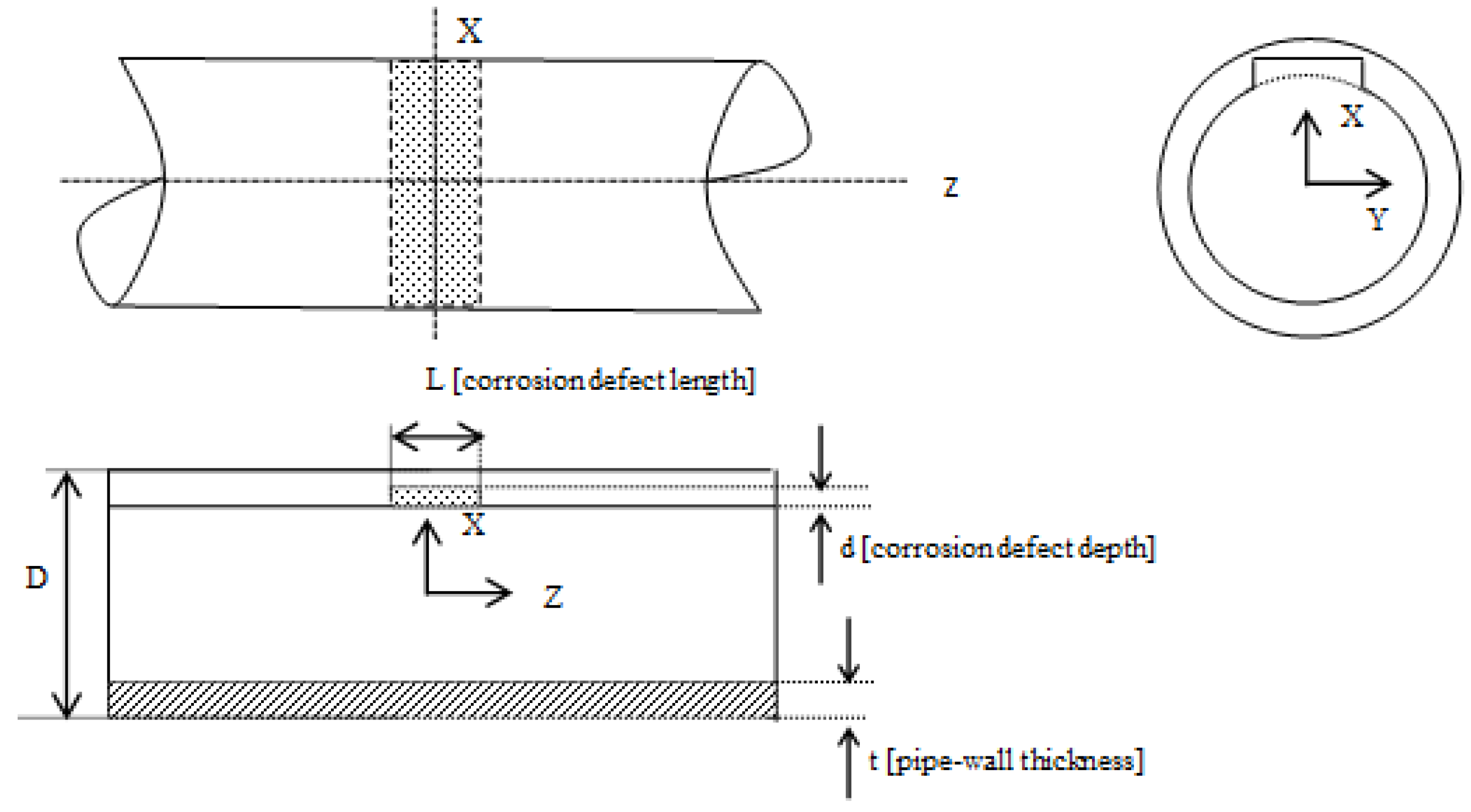
The implementation of this study was based on nonlinear finite element analyses of the strain–stress characteristics of corroded X46 and X52 pipes with diameter (D: 273.05 mm to 836.6 mm), wall thick (t: 5.23 mm to 9.63 mm) and corrosion defect depths (d: 0 mm to 4.62 mm). The analysis also included the corrosion defect length (L) that ranged between 0 mm to 1432.56 mm. It was assumed that the corrosion defects have rectangular cross-sectional areas that uniformly affected the internal pipe-wall thickness in a circumferential direction, as shown in Figure 1.
Static structural components of the ANSYS software was used for the FEM in consideration of the internal pressure exerted by the flowing fluid on the pipe-wall, and the external pressure acting at the fixed ends of the pipeline (Figure 2). These operational forces helped to determine the von Mises stress at the corrosion defect spots on the 1600 mm length pipe used for the developed model. The characteristics of the pipes are shown in Table 1.
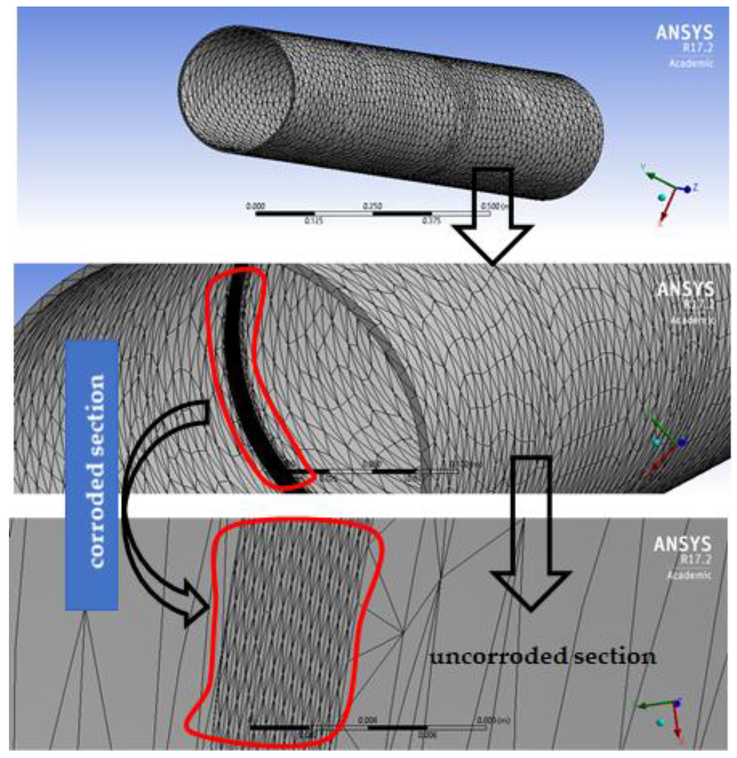
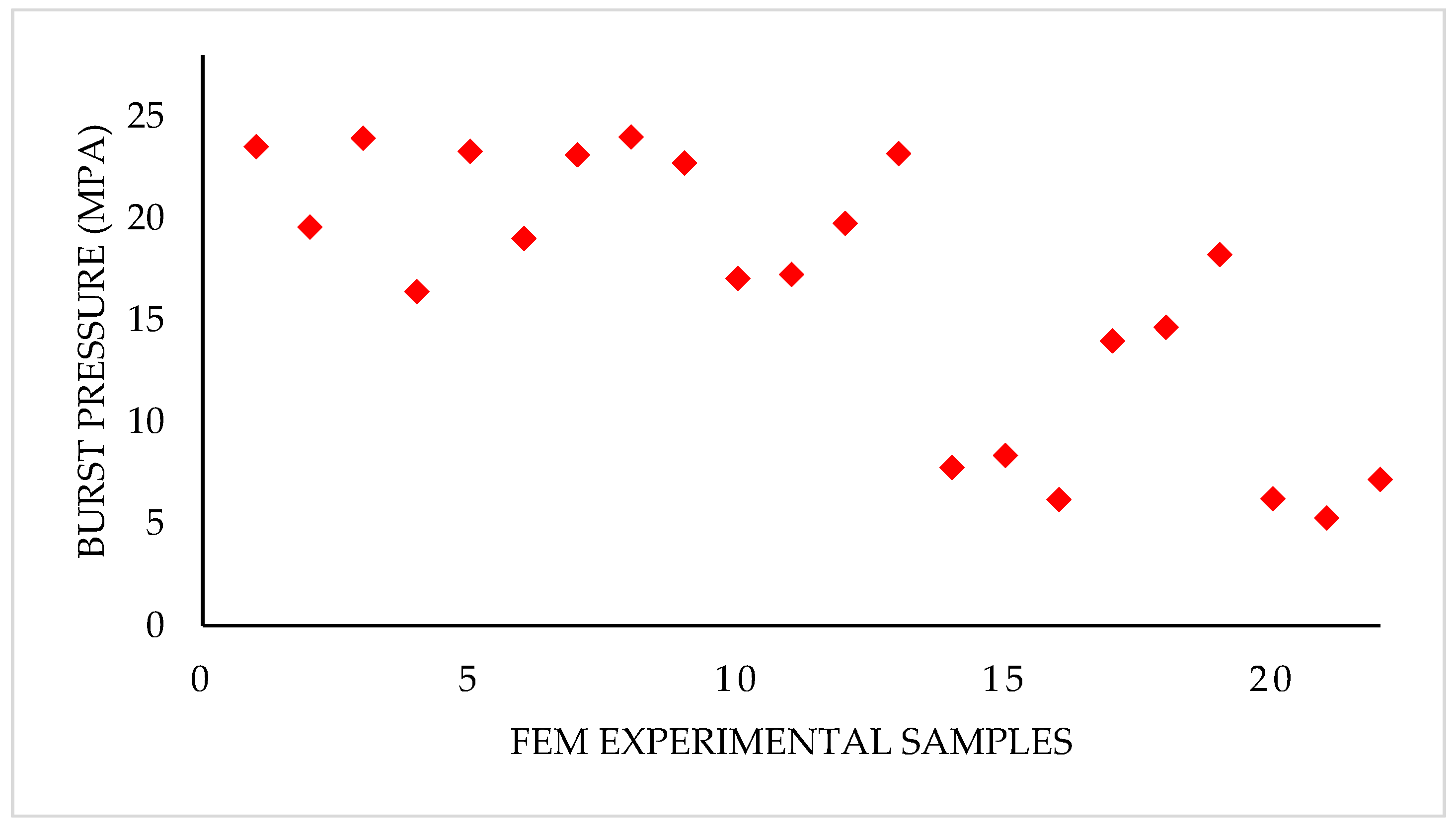
The FEM constructed for one of the X52 pipes, with a diameter of 273.05 mm, thickness of 5.23 mm and defect depth and length of 0.5 mm and 105 mm, respectively, is shown in Figure 3. The model in the figure was created with a total of 149,384 nodes and 80,503 triangular elements that were refined normally at the corrosion section, because there were no distinguishable stress gradients that warranted special refinement [12]. The element size for the mesh ranged from 0.2 mm at the corrosion section to 2 mm at the plane surface of the pipe. The other pipes were modelled with a varying number of nodes and elements, with adequate refinement done at the corrosion sections. A total of 22 FEM analyses were done for both the X46 and X52 pipe grades, to obtain the burst pressures at various corrosion defect depths and lengths (Figure 4).
3. Validation of the Finite Element Modelling Technique
To validate the results of the FEM analysis, experimental results of similar grades of pipes that were conducted with corroded pipeline specimens from different fields were used [13]. The experiments involved 40 specimens obtained over several years through pipeline corrosion investigations in the field. These specimens were used for uniaxial tests that were conducted in both the longitudinal and circumferential directions, by means of sample sizes of 12.7 mm wide and thicknesses representing the original pipe wall thicknesses of the pipelines. Due to the elastoplastic characteristics of the materials [9,10], the investigation of the physical properties of the pipes involved the application of the true stress–strain relationship ((Equations (1) and (2)) and the Ramberg–Osgood principle, for obtaining the total strain (ε) (Equation (3)).
where ɛt, σt, σu, ɛ and n represent the true strain, true stress, tensile strength, total strain and strain hardening exponent, respectively. The elastic modulus (E) of the material was taken to be 207 GPa.
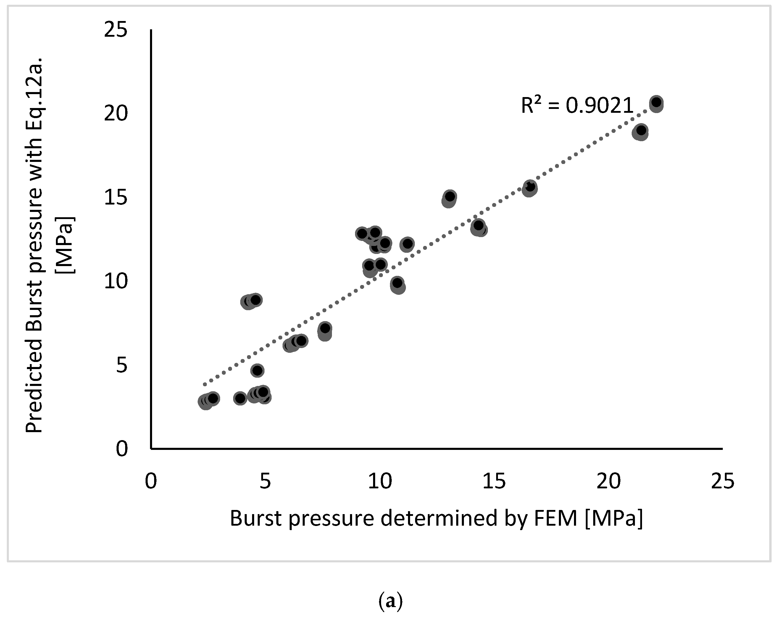
The burst pressures of the pipe specimens were later determined by capping a section of the corroded pipes while applying hydrostatic pressures to determine the burst pressures of the pipes. The comparison of the experimental results and the FEM-predicted results is shown in Figure 5.
The figure shows that a total mean percentage error of 16.14% existed between the FEM results and the experimental results, with a minimum error of −0.33% and maximum error of 34.07% recorded amongst the samples. To further validate the FEM modelling, industry standard models including ASME B31G (modified), RSTRENG, DNV F101, SHELL92 and FITNET FFS [14,15,16,17] were used. These models depend on the corrosion defect geometries—corrosion defect depths and lengths, bending stresses and operating pressures—characterized with numerical and experimental results, for the developed empirical formulas (Equations (4)–(8)). Since most of the analysis on the status of corroded oil and gas pipelines were carried out with these models in the industry, it will be worthwhile testing the robustness of the FEM results against their estimations. Hence, the FEM results were compared with the industry standards model predictions, using Root Mean Square Percentage Error (RMSPE) (Equation (9)); the summary is shown in Table 2.
FITNET FFS:
SHELL92:
DNV-RP-F101:
RSTRENG:
ASME B31G (modified):
where d, L, D, t, σuts and σYS represent corrosion defect depth, corrosion defect length, external diameter of the pipeline, ultimate tensile strength and yield stress, respectively.
Here, the burst pressure from the experimental and industry standard models are represented by ω, the burst pressure predicted with FEM is represented by ℓ, and h represents the number of data tested.
The information in Table 2 shows that the FEM predictions compared favorably with the experimental results and industry standard model predictions, with the RSTRENG model having the best fit amongst the considered industry models and the experimental technique.
The coefficient of determination (R2) of the FEM-predicted burst pressures and the experimental- and industry-model-estimated burst pressures of the pipes are shown in Table 3.
The high coefficient of determination obtained in Table 3 indicates how well the FEM correlates with the industry standards and the experimental results, however, the FEM model has better correlations with the industry models than the experimental technique. This variation may be attributed to flaws in the experiments, which could include measurement and calculation errors that must have been introduced at various times by the diverse people who handled the experiments.
4. Burst Pressure Prediction for Circumferentially-Corroded Pipelines
To predict the burst pressure of the pipes, the FEM technique explained in the previous section was adopted to model the burst pressures of 120 X46 grade pipe of different geometrical configurations and defects (see Table 4).
Since under monotonous loading, the stress concentration is linearly proportional to the applied load [9], an initial internal pressure of 10 MPa was used to determine the stress concentration on the corroded portion of the pipeline. The expected burst pressures of the corroded sections were later determined using the ultimate tensile strength of the material based on the principle of proportionality. It was assumed that the burst pressure of the corroded pipe (Pb) at the limit state is in the form shown in Equation (10) and uniformly affected the corroded section of the pipeline. The stress distribution on the corroded section of the pipe is shown in Figure 6.
If the burst pressure of the pipe with no corrosion defect is given by Pb’, then the burst pressure retention ratio (Rr), which essentially gives an indication of the reliability of the pipe at a given corrosion defect, can be determined with the relationship in Equation (11).
By assuming a linear relationship between the burst pressure and the burst pressure elements d/t, L/D and L/√Dt, a multilinear regression analysis of the burst pressures determined with FEM yielded the relationship shown in Equation (12a,b).
The comparison of the burst pressures predicted with Equation (12a,b) and the FEM data used for the multivariate regression model is shown in Figure 7.
5. Variability of the Retained Strength of the Corroded Pipelines
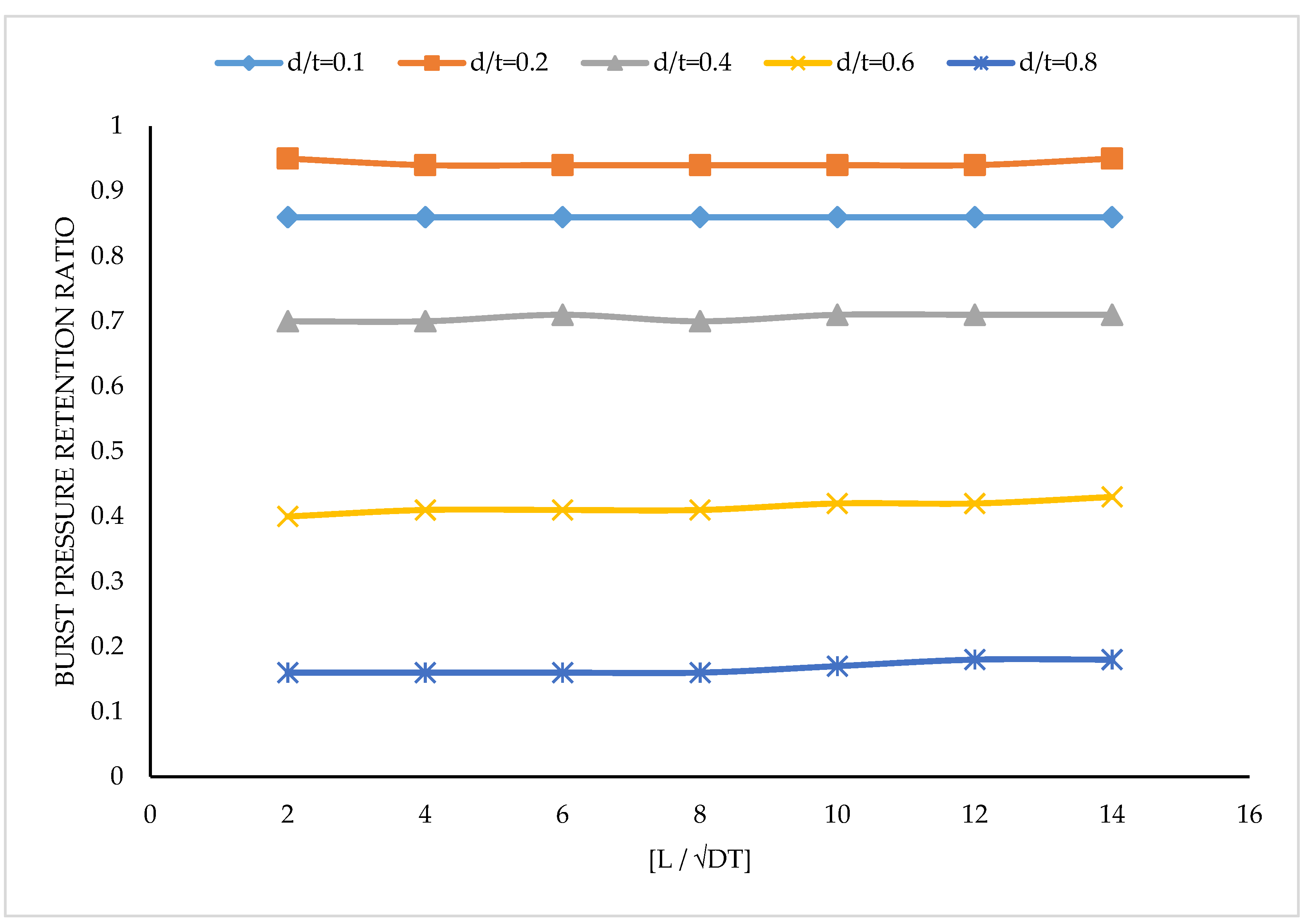
The variability of the retained strength of the corroded pipe as a function of the burst pressure elements, using the model in Equation (12a,b), is exemplified in Figure 8, Figure 9 and Figure 10.
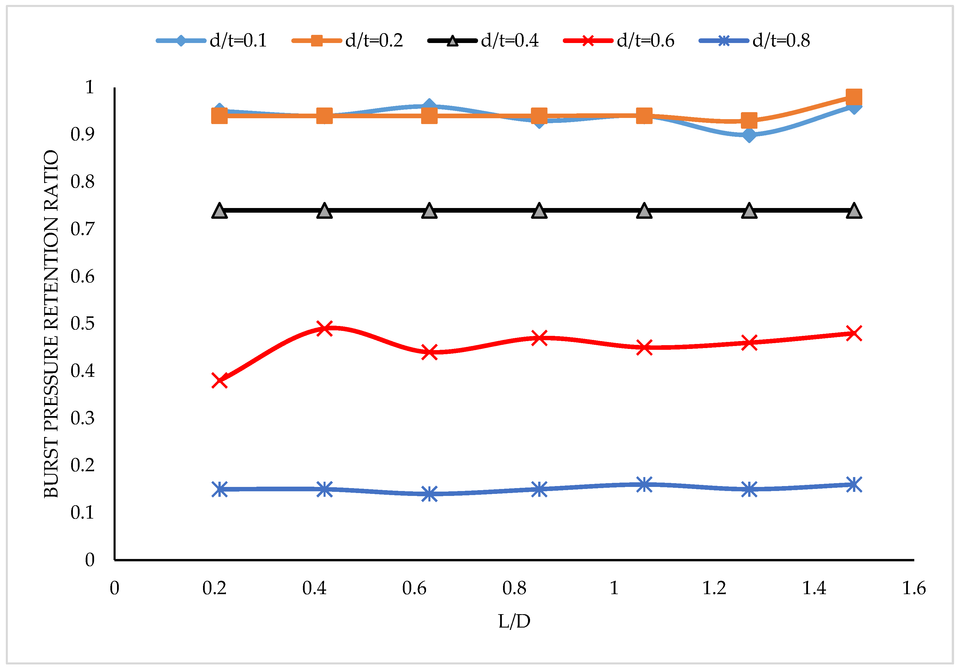
It is evident from the information in Figure 8 that the burst pressure retention ratio (Rr) of the pipes reduced with the increase in d/t, which is similar to the findings of other researchers [5,6,7,8,9]. This scenario was necessitated by the increasing corrosion defect depth, which generally results in increased stress concentration on pipelines [18,19,20]. For a given L/D and L/√Dt (Figure 9 and Figure 10), the retention ratios were fairly steady at each d/t as the L/D and L/√Dt values increased. Again, the increase in d/t saw the Rr decrease for all the values of L/D and L/√Dt, which were also fairly uniform. It can be inferred from these results that pipelines have a lower risk of failure at lesser values of d/t, but increased risks are expected as the value of d/t increases. Again, the limited changes seen in Figure 8 and Figure 9 were indications of the limited influence the corrosion defect length has on the burst pressure of corroded pipelines.
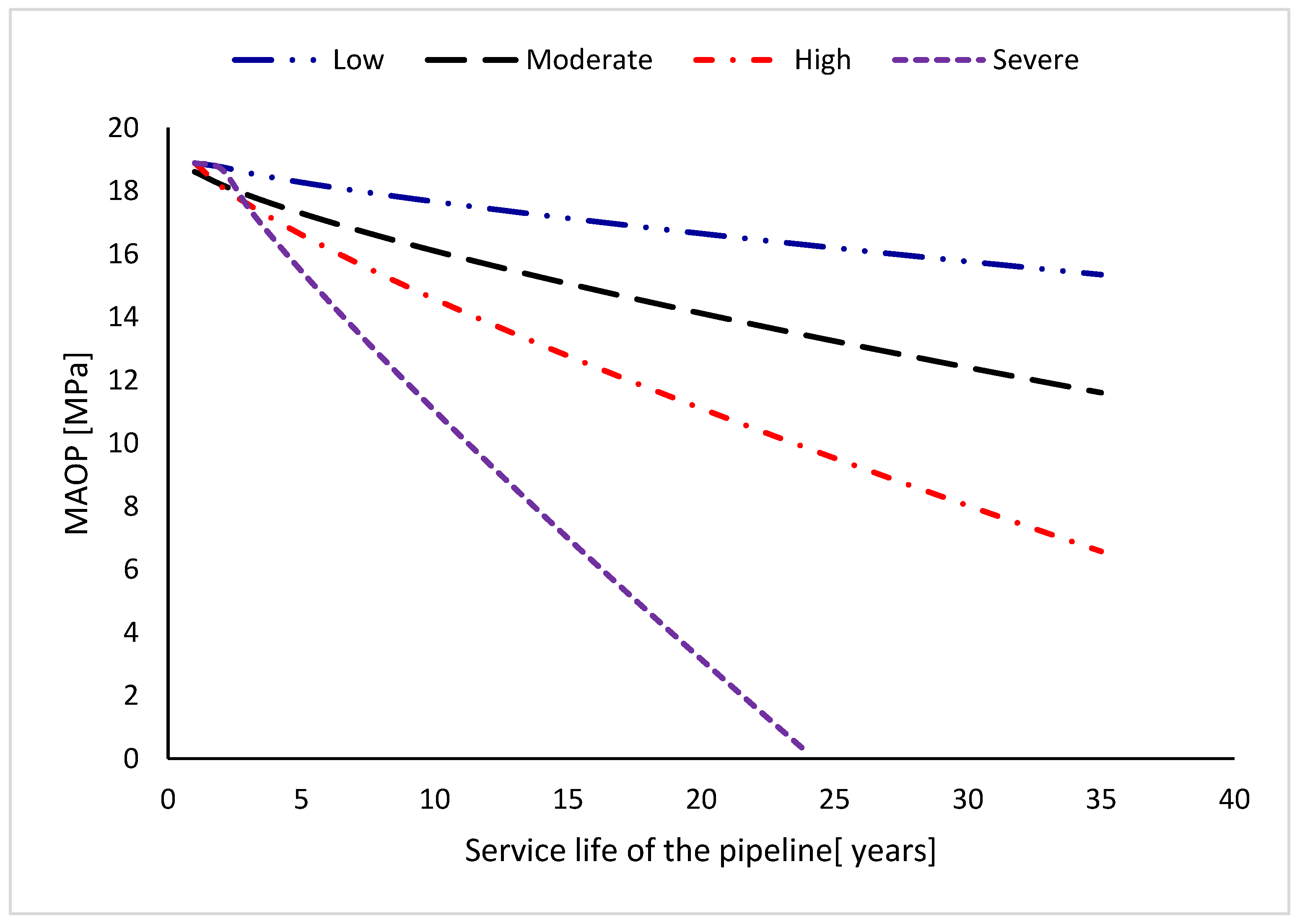
The level of growth of corrosion defect depth of a pipeline in mm/year, determines the category of corrosion the pipeline is undergoing. To this end, if the corrosion defect pit depth growth is less than 0.13 mm/year, it is categorized as low corrosion, whereas a growth rate of between 0.13 mm/year to 0.2 mm/year is mild corrosion. On the other hand, when the corrosion defect pit depth growth is between 0.21 mm/year to 0.38 mm/year, it is said to be undergoing a high corrosion rate, while a growth rate that is above 0.38 mm/year is classified as severe corrosion [21]. If the corrosion defect depth d(t) at time t of a corroded pipeline follows a power model [16,17,18] according to Equation [13], the time of initiation of the corrosion defects (tini) for different corrosion categories are low corrosion (tini = 1.56 years), mild corrosion (tini = 0.58 years), high corrosion (tini = 1.03 years) and severe corrosion (tini = 1.89 years) [22]. In this case, the burst pressure at different lifecycle durations and various corrosion categories can be computed with Equations (12a,b). If the burst pressure of the pipeline computed with Equations (12a,b) represents the Maximum Allowable Operating Pressure (MAOP) at any given time in the lifecycle of the asset, and the maximum corrosion defect depth growth dmax(t) can be computed with Equation (14) [23], then the MAOP for X46 grade of pipeline with 323.6 mm diameter will be patterned according to Figure 11.
where k and α represent the proportionality and exponential constants, respectively.
An increase in the service life of corroded pipelines generally results in a decrease of the burst pressures, with the severe corrosion category showing the worst decrease amongst the corrosion categories, because of the very high rate of pipe wall thickness loss. The estimated MAOP in this figure is indicative, because the existence of other defects on the corroded sections of the pipeline will alter the estimated values of the burst pressures. Notwithstanding, the model developed in this study provides valuable information for flowline design and pipeline integrity management.
6. Conclusions
This research presented a finite element modelling (FEM) technique that utilized the static structural component of ANSYS to predict the burst pressure of internally, circumferentially-corroded pipelines, under the influence of internal operating pressure and external pressure with a fixed support. The FEM-estimated burst pressures of X46 and X52 grade pipeline materials were compared with the experimental and industry standard models—FITNET FFS, SHELL 92, DNV RP-F101, ASME B31G (modified) and RSTRENG—using RMSPE. The values of the RMPSE were experimental: 20.4%, FITNET FFS: 15.97%, SHELL 92: 7.24%, DNV F101: 13.07%, RSTRENG: 7.06% and ASME B31G (modified): 10.97%. The coefficient of determination (R2) of the FEM-predicted burst pressures as compared to the experimental and industry-based models were experimental (R2 = 0.8924), FITNET FFS (R2 = 0.7932), SHELL 92 (R2 = 0.9769), DNV F101 (R2 = 0.9592), RSTRENG (R2 = 0.9813) and ASME B31G (modified) (R2 = 0.9812). A multivariate regression model was developed using 120 FEM-predicted burst pressures and other variables—d/t, L/D and L/√Dt—while the burst pressure retention ratio (Rr) that indicated the reliability of the pipes was computed as the ratio of the burst pressure of the corroded pipe section to a non-corroded section.
As expected, the reliability of the pipes were found to decrease with an increase in the d/t, but the increase in L on its own did not result in significant changes in the reliability and risk exposure levels of the pipes. The FEM-developed multivariate model was also used for the estimation of the expected Maximum Allowable Operating Pressure (MAOP) of pipelines that were undergoing low, mild, high and severe corrosion rates, using corrosion defect growth models. Based on the robustness of this study, as shown by the results, the developed model will be a viable instrument for the estimation of the remaining useful life of aged corroded pipelines and will be a very helpful tool for designing flowlines and managing pipeline integrity. However, when other defects exist in the pipeline, the estimated burst pressures will only be marginal because the influence of the unknown or known defects that were not considered in the model will affect the results.
Conflicts of Interest
The author has no conflict of interest.
References
- Kaminski, M. The Stochastic Perturbation Method for Computational Mechanics; John Wiley & Sons, Ltd.: West Sussex, UK, 2013. [Google Scholar]
- Kamiński, M.M.; Świta, P. Generalized stochastic finite element method in elastic stability problems. Comput. Struct. 2011, 89, 1241–1252. [Google Scholar] [CrossRef]
- Chen, Y.; Zhang, H.; Zhang, J.; Li, X.; Zhou, J. Failure analysis of high strength pipeline with single and multiple corrosions. Mater. Des. 2015, 67, 552–557. [Google Scholar] [CrossRef]
- Bai, Y.; Song, R. Fracture assessment of dented pipes with cracks and reliability-based calibration of safety factor. Int. J. Press. Vessels Pip. 1997, 74, 221–229. [Google Scholar] [CrossRef]
- Wang, N.; Zarghamee, M. Evaluating Fitness-for-Service of Corroded Metal Pipelines: Structural Reliability Bases. J. Pipeline Sys. Eng. Pract. 2014, 5, 04013012. [Google Scholar] [CrossRef]
- Xue, J. A non-linear finite-element analysis of buckle propagation in subsea corroded pipelines. Finite Elem. Anal. Des. 2006, 42, 1211–1219. [Google Scholar] [CrossRef]
- Yang, Z.; Liu, D.; Zhang, X. Finite element method analysis of the stress for line pipe with corrode groove during outdoor storage. Acta Metall. Sin. Engl. Lett. 2013, 26, 188–198. [Google Scholar] [CrossRef]
- Netto, T.A.; Ferraz, U.S.; Estefen, S.F. The effect of corrosion defects on the burst pressure of pipelines. J. Constr. Steel Res. 2005, 61, 1185–1204. [Google Scholar] [CrossRef]
- Ma, B.; Shuai, J.; Liu, D.; Xu, K. Assessment on Failure Pressure of High Strength Pipeline with Corrosion Defects. Eng. Fail. Anal. 2013, 32, 209–219. [Google Scholar] [CrossRef]
- Zhu, X.K.; Leis, B.N. Theoretical and numerical predictions of burst pressure of pipelines. J. Press. Vessel Technol. 2007, 129, 644–652. [Google Scholar] [CrossRef]
- Xu, L.Y.; Cheng, Y.F. Development of a finite element model for simulation and prediction of mechanoelectrochemical effect of pipeline corrosion. Corros. Sci. 2013, 73, 150–160. [Google Scholar] [CrossRef]
- Chiodo, M.S.; Ruggieri, C. Failure assessments of corroded pipelines with axial defects using stress-based criteria: numerical studies and verification analyses. Int. J. Press. Vessels Pip. 2009, 86, 164–176. [Google Scholar] [CrossRef]
- Cronin, D.S. Assessment of Corrosion Defects in Pipelines; University of Waterloo: Waterloo, ON, Canada, 2001. [Google Scholar]
- Ossai, C.I.; Boswell, B.; Davies, I.J. Pipeline failures in corrosive environments–A conceptual analysis of trends and effects. Eng. Fail. Anal. 2015, 53, 36–58. [Google Scholar] [CrossRef]
- Cosham, A.; Hopkins, P.; Macdonald, K.A. Best practice for the assessment of defects in pipelines—Corrosion. Eng. Fail. Anal. 2007, 14, 1245–1265. [Google Scholar] [CrossRef]
- American Society of Mechanical Engineers. Manual for Determining the Remaining Strength of Corroded Pipelines; ASME B31G; American Society of Mechanical Engineers: New York, NY, USA, 2009. [Google Scholar]
- Qian, G.; Niffenegger, M.; Zhou, W.; Li, S. Effect of correlated input parameters on the failure probability of pipelines with corrosion defects by using FITNET FFS procedure. Int. J. Press. Vessel. Pip. 2013, 105, 19–27. [Google Scholar] [CrossRef]
- Ossai, C.I.; Boswell, B.; Davies, I.J. Estimation of internal pit depth growth and reliability of aged oil and gas pipelines—A Monte Carlo simulation approach. Corrosion 2015, 71, 977–999. [Google Scholar] [CrossRef]
- Velázquez, J.; Caleyo, F.; Valor, A.; Hallen, J. Predictive model for pitting corrosion in buried oil and gas pipelines. Corrosion 2009, 65, 332–342. [Google Scholar]
- Katano, Y.; Miyata, K.; Shimizu, H.; Isogai, T. Predictive model for pit growth on underground pipes. Corrosion 2003, 59, 155–161. [Google Scholar] [CrossRef]
- NACE. Preparation, Installation, Analysis and Interpretation of Corrosion Coupons in Oilfield Operations; NACE standard RP0775; NACE international: Houston, TX, USA, 2005. [Google Scholar]
- Ossai, C.I.; Boswell, B.; Davies, I.J. Markov chain modelling for time evolution of internal pitting corrosion distribution of oil and gas pipelines. Eng. Fail. Anal. 2016, 60, 209–228. [Google Scholar] [CrossRef]
- Ossai, C.I.; Boswell, B.; Davies, I.J. Predictive modelling of internal pitting corrosion of aged non-piggable pipelines. J. Electrochem. Soc. 2015, 162, C251–C259. [Google Scholar] [CrossRef]
Figure 1.
Schematic of a circumferential corrosion defect of a pipe.

Figure 2.
Finite Element Modelling (FEM) supporting and acting pressures on the modelled 1600 mm long X46 and X52 pipe.
Figure 2.
Finite Element Modelling (FEM) supporting and acting pressures on the modelled 1600 mm long X46 and X52 pipe.

Figure 3.
Nonlinear FEM for X52 grade pipe of 273.05 mm diameter, 5.23 mm thick, d/t of 0.1 and L of 105 mm.
Figure 3.
Nonlinear FEM for X52 grade pipe of 273.05 mm diameter, 5.23 mm thick, d/t of 0.1 and L of 105 mm.

Figure 4.
Summary of FEM estimated burst pressures for the pipes—samples 1 to 13 are for X46 (D: 321.56 mm to 324.1 mm), samples 14 to 16 are for X46 (D: 836.6 mm), samples 17 to 19 are for X52 (D: 273.05 mm) and samples 20 to 22 are for X52 (D: 611.35 mm to 612.54 mm).
Figure 4.
Summary of FEM estimated burst pressures for the pipes—samples 1 to 13 are for X46 (D: 321.56 mm to 324.1 mm), samples 14 to 16 are for X46 (D: 836.6 mm), samples 17 to 19 are for X52 (D: 273.05 mm) and samples 20 to 22 are for X52 (D: 611.35 mm to 612.54 mm).

Figure 5.
Comparison of FEM analysis with experimental results for the 22 samples of X46 and X52 grade pipes.
Figure 5.
Comparison of FEM analysis with experimental results for the 22 samples of X46 and X52 grade pipes.
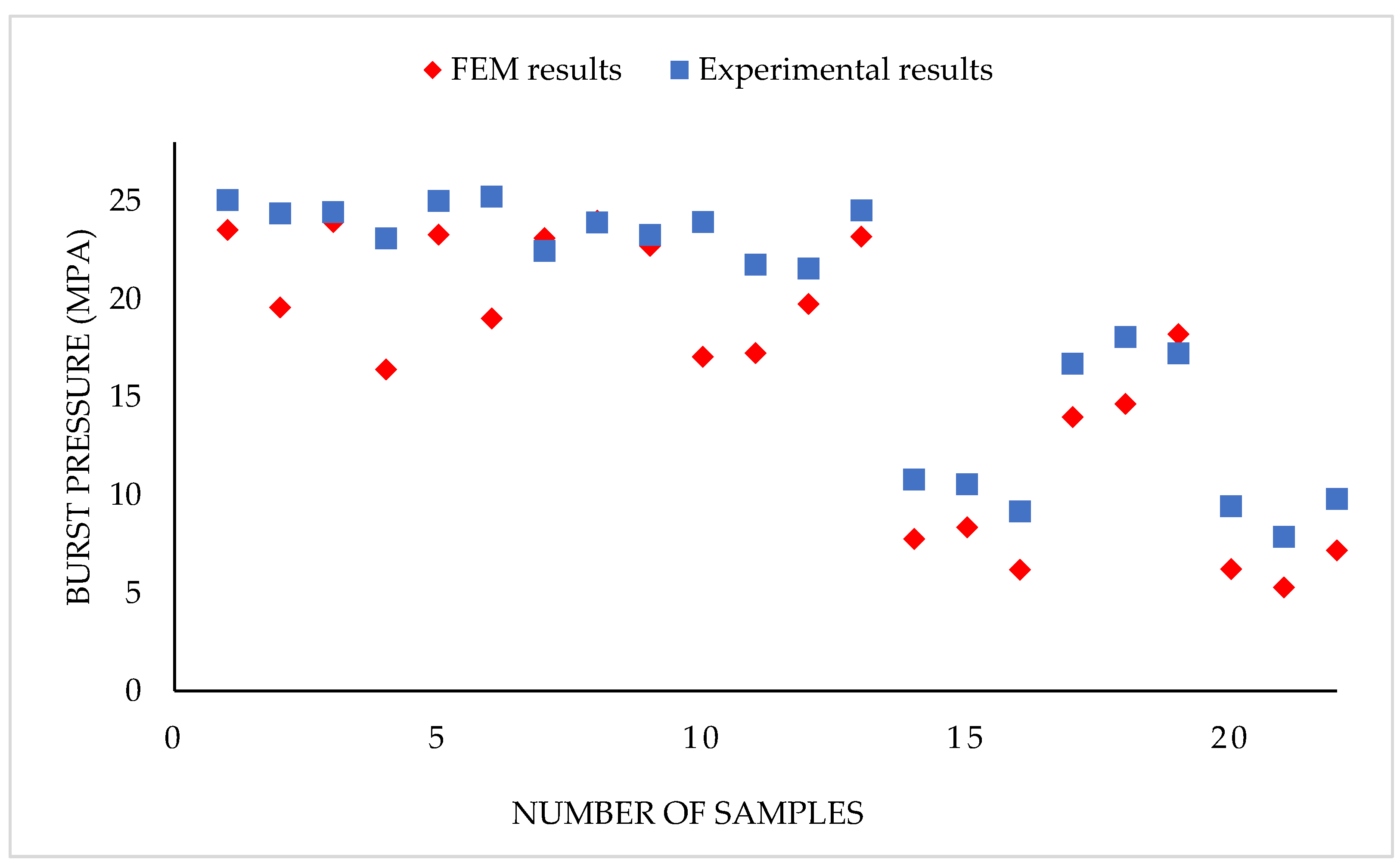
Figure 6.
Stress distribution around the corrosion defect section and the non-corroded sections of the X46 grade pipe with 273.05 mm diameter, 5.23 mm thick, d/t of 0.1 and L of 105 mm.
Figure 6.
Stress distribution around the corrosion defect section and the non-corroded sections of the X46 grade pipe with 273.05 mm diameter, 5.23 mm thick, d/t of 0.1 and L of 105 mm.

Figure 7.
(a) Comparison of the FEM estimation (Pb) with the estimation from Equation (12a). (b) Comparison of the FEM estimation (Pb) with the estimation from Equation (12b).
Figure 7.
(a) Comparison of the FEM estimation (Pb) with the estimation from Equation (12a). (b) Comparison of the FEM estimation (Pb) with the estimation from Equation (12b).

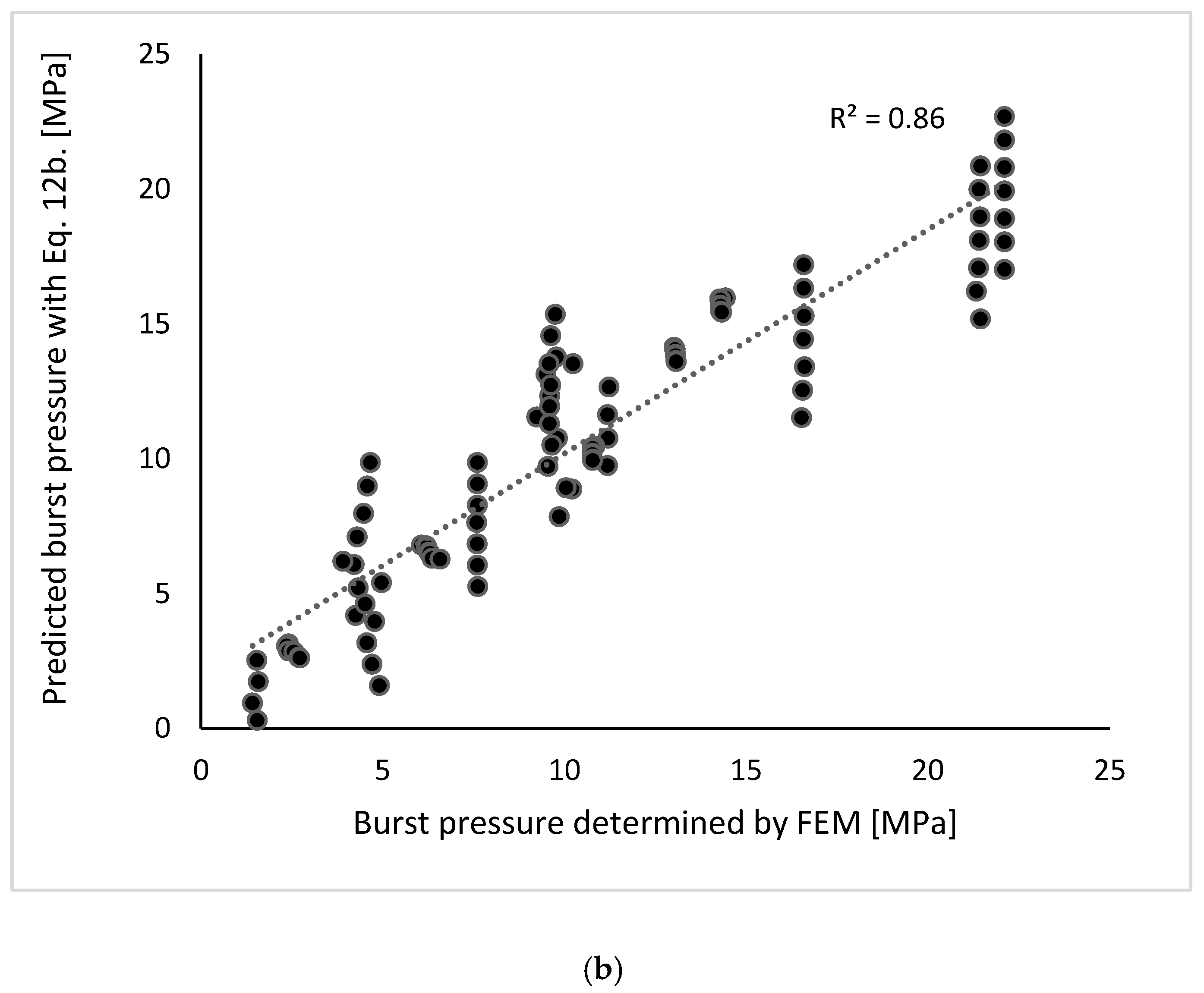
Figure 8.
Variation of the burst pressure retention ratio with d/t for 323.6 mm diameter and 8.51 mm thick pipe for various corrosion defect lengths mm.
Figure 8.
Variation of the burst pressure retention ratio with d/t for 323.6 mm diameter and 8.51 mm thick pipe for various corrosion defect lengths mm.
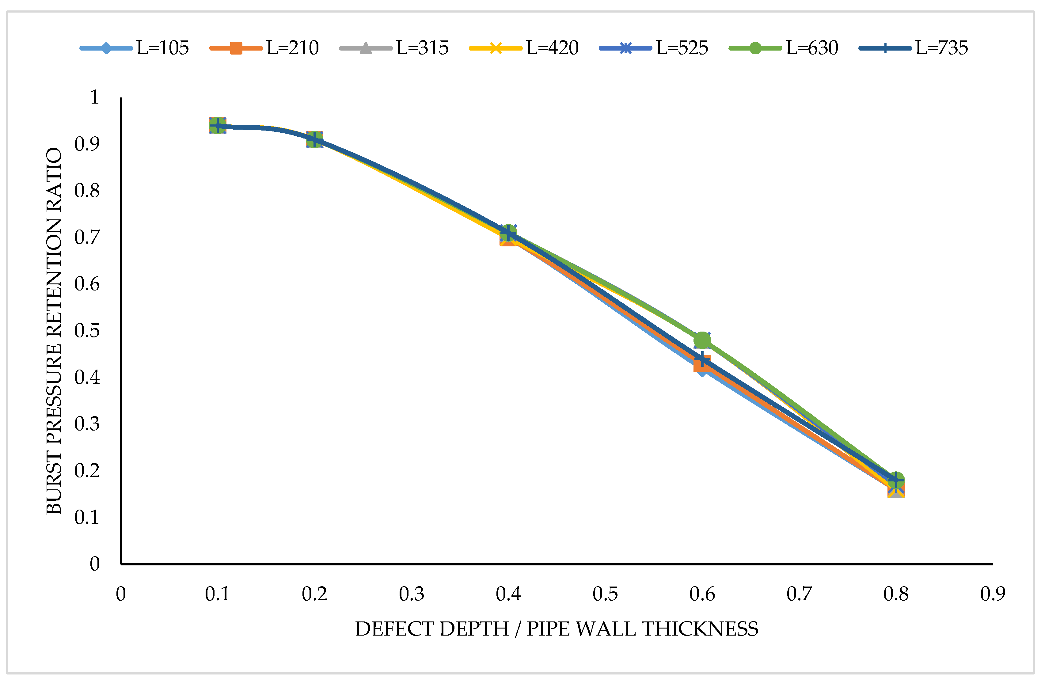
Figure 9.
Variation of the burst pressure retention ratio with L/√Dt for 534.4 mm diameter and 8.71 mm thick pipe for various d/t.
Figure 9.
Variation of the burst pressure retention ratio with L/√Dt for 534.4 mm diameter and 8.71 mm thick pipe for various d/t.

Figure 10.
Variation of the burst pressure retention ratio with L/D for 863.6 mm diameter and 9.63 mm thick pipe for various d/t.
Figure 10.
Variation of the burst pressure retention ratio with L/D for 863.6 mm diameter and 9.63 mm thick pipe for various d/t.

Figure 11.
Predicted Maximum Allowable Operating Pressure (MAOP) for a 323.6 mm diameter and 8.51 mm thick pipeline with a 105 mm-long corrosion defect and an ultimate tensile strength of 469.27 MPa using Equation (12a).
Figure 11.
Predicted Maximum Allowable Operating Pressure (MAOP) for a 323.6 mm diameter and 8.51 mm thick pipeline with a 105 mm-long corrosion defect and an ultimate tensile strength of 469.27 MPa using Equation (12a).


Table 1.
Characteristics of the pipes used for Finite Element Modelling (FEM).
| Grade | D (mm) | t (mm) | d (mm) | L (mm) | σu (MPa) | σY (MPa) | NOS |
|---|---|---|---|---|---|---|---|
| X46 | 321.56–324.01 | 8.33–8.74 | 0.00–3.30 | 0–144.78 | 469.27 | 356.38 | 13 |
| X46 | 863.6 | 9.37–9.63 | 3.00–4.62 | 91.44–408.94 | 508.01 | 400.24 | 3 |
| X52 | 273.05 | 5.23–5.28 | 0.00–1.85 | 0–408.94 | 502.25 | 388.7 | 3 |
| X52 | 611.35–612.54 | 6.40–6.55 | 2.57–3.56 | 901.7–1371.6 | 533.82 | 402.52 | 3 |
σu: Ultimate tensile strength; σy: Yield stress, NOS: number of samples.
Table 2.
Summary of the Root Mean Square Percentage Error (RMSPE) of X46 and X52 grade pipes’ FEM-estimated burst pressures compared with the experimental and industry standard models (EISM) estimations.
Table 2.
Summary of the Root Mean Square Percentage Error (RMSPE) of X46 and X52 grade pipes’ FEM-estimated burst pressures compared with the experimental and industry standard models (EISM) estimations.
| EISM | Experimental | FITNET FFS | SHELL 92 | DNV F101 | RSTRENG | ASME-mod |
|---|---|---|---|---|---|---|
| RMSPE | 20.4% | 15.97% | 7.24% | 13.07% | 7.06% | 10.97% |
Table 3.
Summary of the coefficient of determination (R2) of X46 and X52 grade pipe burst pressure as compared with the experimental and industry standard models (EISM).
Table 3.
Summary of the coefficient of determination (R2) of X46 and X52 grade pipe burst pressure as compared with the experimental and industry standard models (EISM).
| EISM | Experimental | FITNET FFS | SHELL 92 | DNV F101 | RSTRENG | ASME B31G (mod) |
|---|---|---|---|---|---|---|
| R2 | 0.8924 | 0.7932 | 0.9769 | 0.9592 | 0.9813 | 0.9812 |
Table 4.
Summary of pipeline geometry used for the prediction of burst pressure using FEM.
| D (mm) | t (mm) | σu (MPa) | σY (MPa) | d (mm) | L (mm) | NOS |
|---|---|---|---|---|---|---|
| 323.6 | 8.51 | 469.27 | 356.38 | 0–6.81 | 105–735 | 40 |
| 534.4 | 8.71 | 491.65 | 373.21 | 0–6.97 | 136–955 | 40 |
| 863.6 | 9.63 | 508.01 | 400.24 | 0–7.70 | 182–1277 | 40 |
© 2017 by the author. Licensee MDPI, Basel, Switzerland. This article is an open access article distributed under the terms and conditions of the Creative Commons Attribution (CC BY) license (http://creativecommons.org/licenses/by/4.0/).
Share and Cite
MDPI and ACS Style
Ossai, C.I. Finite Element Modelling and Retained Life Estimation of Corroded Pipelines in Consideration of Burst Pressures—A Fractural Mechanics Approach. Infrastructures 2017, 2, 15. https://doi.org/10.3390/infrastructures2040015
AMA Style
Ossai CI. Finite Element Modelling and Retained Life Estimation of Corroded Pipelines in Consideration of Burst Pressures—A Fractural Mechanics Approach. Infrastructures. 2017; 2(4):15. https://doi.org/10.3390/infrastructures2040015
Chicago/Turabian StyleOssai, Chinedu I. 2017. "Finite Element Modelling and Retained Life Estimation of Corroded Pipelines in Consideration of Burst Pressures—A Fractural Mechanics Approach" Infrastructures 2, no. 4: 15. https://doi.org/10.3390/infrastructures2040015