Improving MMS Performance during Infrastructure Surveys through Geometry Aided Design

Abstract

A Mobile Mapping System (MMS) equipped with laser scanners can collect large volumes of LiDAR data in a short time frame and generate complex 3D models of infrastructure. The performance of the automated algorithms that are developed to extract the infrastructure elements from the point clouds and create these models are largely dependent on the number of pulses striking infrastructure in these clouds. Mobile Mapping Systems have evolved accordingly, adding more and higher specification scanners to achieve the required high point density, however an unanswered question is whether optimising system configuration can achieve similar improvements at no extra cost. This paper presents an approach for improving MMS performance for infrastructure surveys through consideration of scanner orientation, scanner position and scanner operating parameters in a methodology referred to as Geometry Aided Design. A series of tests were designed to measure point cloud characteristics such as point density, point spacing and profile spacing. Three hypothetical MMSs were benchmarked to demonstrate the benefit of Geometry Aided Design for infrastructure surveys. These tests demonstrate that, with the recommended scanner configuration, a MMS, operating one high specification scanner and one low specification scanner, is capable of comparable performance with two high-end systems when benchmarked against a selection of planar, multi-faced and cylindrical targets, resulting in point density improvements in some cases of up to 400%.

1. Introduction

The high volumes of density spatial data produced by Mobile Mappinh Systems (MMSs) [1,2] result in increased processing times. Manual interpretation and extraction of features in the dataset can be very time consuming, and as a result one of the aims of the research community is to develop automated extraction of features in the point cloud. These algorithms can potentially reduce or eliminate the amount of manual interrogation of the data. Automated algorithms have been developed to identify trees, poles, road edges and are an important research question [3,4,5,6,7,8,9]. However, one important consideration when designing each algorithm is the characteristics of the point cloud that will enable successful extraction of a feature. Studies demonstrate [10,11,12] that a minimum number of laser points and scan profiles are required on cylindrical objects to accurately recognise those features and laser point cloud density directly impacts on the accuracy [13] of the resulting extracted model.

Point density is traditionally quoted in points per m${}^2$, an unsuitable description for a 3 Dimensional (3D) object [14]. This issue has been explored [15] for terrestrial and aerial LiDAR and ways to define point density for 3D data and the importance of achieving a sufficient point density on data processing identified. It is difficult to calculate what point density a MMS will be capable of and this paper will further the body of knowledge on MMS performance. MMS survey specifications have been created [16,17] to inform surveyors as to what is required from a survey; and recent publications [18] have improved on this by subdividing point density into coarse, intermediate, and fine point cloud density. Further recommendations are that a continuous, color-coded point density map with summary statistics for the survey area is included as a deliverable. These guidelines provide tabular information on what point spacing is required to achieve a specific level of point density, but does not define what MMS hardware, hardware configuration or operating parameters are required to achieve that point spacing. At present there are no generic, robust, easily repeatable methods for quantifying or assessing the point density exhibited by MMSs.

This paper will apply an existing methodology to quantifying MMS point clouds, thereby improving MMS performance through the following innovative MMS configurations and operating parameters:

• Utilising both axes of the MMS for the second scanner to reduce scan range.
• Increasing the length of scan profile that intersects with a target by changing the vertical orientation of the scanner.
• Limiting the Field of View (FOV) of the scanner to decrease the angular step width between subsequent laser pulses.

2. Background and Related Work

There are many types of MMS and they are capable of varied performances, and although a number of studies have explored this in the past, the innovative method proposed in this paper will allow MMSs to be explored in greater detail, enabling easier, multi-system benchmarking using non-default configurations.

2.1. MMS Types

An MMS operating laser scannerz evolved from single scanner systems to the dual scanner systems such as those leading the market today [19,20,21,22]. These scanners operate in the ‘butterfly’ configuration, with the two scanners positioned symmetrically at the rear of the vehicle, angled to either side of the vehicle. The dual scanner systems on the market incorporate vertical and horizontal rotations of the scanner to ensure that the laser scanner will be capable of surveying structures that are perpendicular to the direction of travel. These scanner orientations also directly impact the angle at which the scan plane intersects with the surrounding environment and also changes the range to the target (Figure 1a). Horizontal scanner rotations result in an increased range to the target on both sides of the vehicle, as displayed in Figure 1b, whereas vertical orientations of the scanner result in an increased range to the road surface underneath the MMS. Incorporating both orientations in both axes, horizontal and vertical, results in an increased range to the road surface and also to roadside targets, as displayed in Figure 1c. There is therefore a clear need to investigate the influence that scanner orientations have when surveying roadside infrastructure and to identify the optimal configuration. MMS performance analysis and benchmarking enables this.

2.2. System Benchmarking

A number of studies have assessed the performance of specific MMSs. A FARO Terrestrial Laser Scanner (TLS) was installed on a MMS to measure profile and point spacing at different ranges, velocities and scan frequencies [23]. This data can be used to estimate point spacing for subsequent FARO surveys. Similar tests have also been performed [24] with a Leica HDS 4500 locked in one axis and operating in profile mode. Hardware manufacturers such as Riegl provide detailed graphs [21] plotting the point density a user can expect at different vehicle velocities using different scanner settings and at different target ranges that is very useful in the mission planning stage, however it is difficult to compare MMSs using these methods. LiDAR simulations have been used for investigating multiple aerial systems, such as [25] and other simulators have been designed, such as that by [26] for algorithm development, system validation and error assessment for aerial and terrestrial systems. Simulators are useful tools for assessing MMS coverage over wide areas, or for algorithm development but are not designed for analysis at the target level. A dedicated MMS simulation was designed by [14] to measure the mean point density for large areas of a scene. This study provided recommendations for specific MMS configurations to minimise data shadows for terrestrial MMS surveys, however it did not explore each of the point cloud characteristics for infrastructure surveys, such as target variable point spacing, profile angle, profile spacing, etc. Comprehensive real-world benchmarking tests have also been performed on a permanent test field using a series of MMSs and the default hardware configuration [27], however this method requires access to a range of real-world MMSs. The innovative method for system benchmarking that is proposed in this paper enables any number of hypothetical configurations to be explored rapidly accurately.

2.3. MIMIC

The MobIle Mapping point densIty Calculator (MIMIC) has been designed and developed by researchers at the National Centre for Geocomputation, Maynooth University. MIMIC calculates point distribution and point density through use of 3D surface normals and 2D geometric formulae. MIMIC calculates the theoretical position of each laser pulse on the target surface, and therefore random events such as occlusions, multiple returns, different surface types and GNSS/IMU errors are not modelled. MIMIC and the multiple variables that need to be considered when designing a system to calculate point density were first introduced in [28], and the formulae and processes used for its design have been incrementally validated using a selection of real-world MMS point clouds [29,30,31,32,33,34]. MIMIC is compatible with different scanner hardware, scanner configurations, vehicle variables and target variables and provides detailed information in tabular or graphical format (using interpolation techniques designed in [35]) to help visualise point and profile distribution.

3. Enabling MMS Performance Improvements through Geometry Aided System Design

MIMIC enables a methodology for benchmarking MMS performance developed at Maynooth University, entitled, Geometry Aided Design (GAD). This paper will use GAD to demonstrate the benefit of utilising both the X and Y axes of the MMS for scanner position, identifying the optimum vertical orientation of the scanner and assessing the influence of limiting the FOV of the scanner.

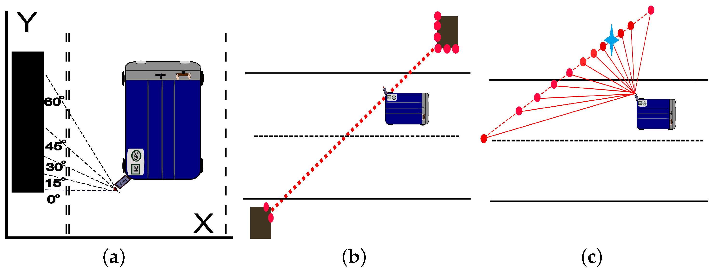
3.1. Scanner Position

One potential variable of MMS design is the horizontal position of the scanner on the MMS. The position of the scanner can be varied in the XY axes, or in the X or Y axes, as illustrated in Figure 2a with Scanners 1–4. The configuration can be adapted for any mobile platform, such as a car or trailer and is not specific to the van illustrated in this image. The impact that changing the scanner location in either axis has on point density is examined in the following section. It is important to note that changes in the location of the scanner assumed no obstructions caused by the vehicle body or the navigation sensors. Scanners located near the extremities of the MMS must be able to avoid obstructions from the vehicle.

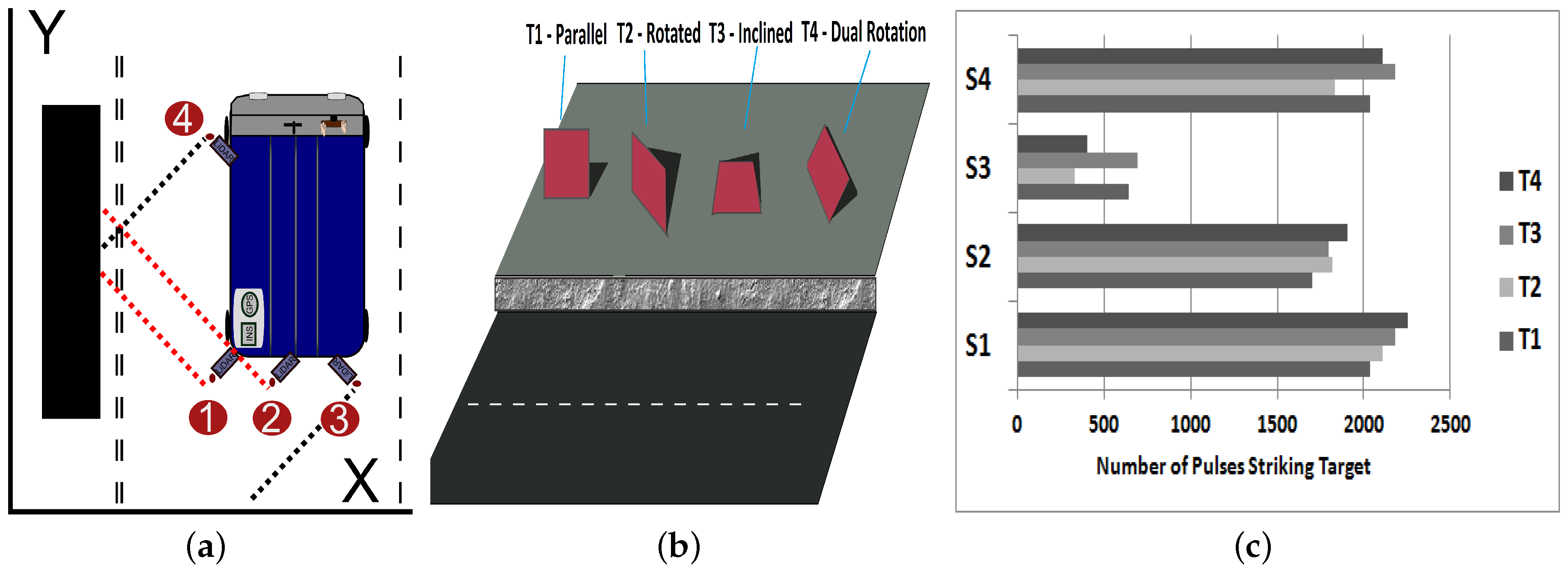
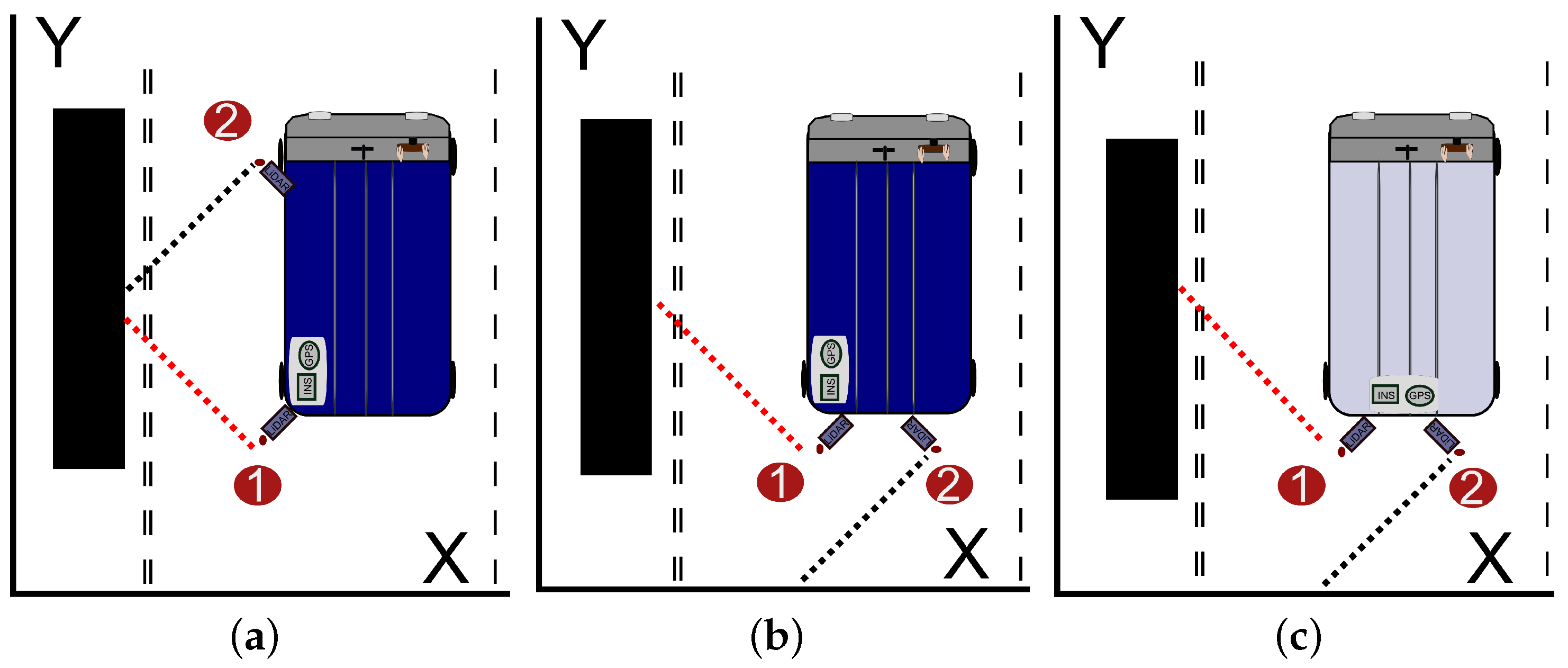
3.1.1. Offset Scanner on Vehicle X Axis (Position 1 and 2)

For Scanners 1 and 2, a change in the horizontal axis of the scanner, as illustrated in Figure 2a, is analogous with an increase in the horizontal range to the target. These tests quantify the effect that altering the position of the scanner on the X axis of the MMS has on point density. The scanners are positioned in the same XY coordinate system as the vehicle and each scanner pivots around the base in horizontal and vertical for all orientation changes. Full detail on the rotation process in MIMIC is provided in [32]. The two scanners used in these tests are orientated at a 45${}^{°}$ horizontal and a 45${}^{°}$ vertical rotation matching the generic scanner orientation of the MMS designed at the NCG, the XP1 [28]. The system designed at the NCG operates a Riegl VQ250 scanner, a 300 kHz pulse repetition rate (PRR) and 100 Hz mirror speed. An offset of 1 m was defined for Scanner 2 and a 2 m × 1 m target and a vehicle velocity of 50 km/h were also specified. Four different target orientations were applied in these tests (Figure 2b); the first target is parallel to the direction of travel, whereas the second is rotated horizontally, the third inclined vertically and the fourth target is a combination of both horizontal and vertical angular changes. Including variations in target orientation and inclination is essential to robustly assess the diverse MMSs in these tests, as the orientation of the target will increase and decrease the range to target differently across the target, as demonstrated in [33].

The results of these tests are displayed in Figure 2c. For each target, Scanner 1 consistently outperforms Scanner 2, returning 333 more points than Scanner 2 for the parallel target. The results show that a 1m change in horizontal scanner position in the X axis results in approximately an average 16% decrease in point density on each target. Scanners that are removed from the extremities of the vehicle will not be capable of comparable point densities.

3.1.2. Common Commercial Dual Scanner Configuration (Position 1 and 3)

A common configuration [20,21] for dual scanner MMSs is a symmetrical second scanner offset in the X axis, a configuration illustrated by Scanners 1 and 3 in Figure 2a. To assess the effect of this orientation on point density, the same tests were repeated, however, to eliminate the effect of two different X positions on the point density, no scanner offset was applied to Scanner 3. Scanner 1 has significantly outperformed Scanner 3 in these tests. For a parallel target, a negatively rotated scanner (away from the target) such as Scanner 3 exhibits a 68% drop in point density when compared to Scanner 1. The underlying reason for the lower point density for Scanner 3 in these tests is the increased measurement range for Scanner 3 arising from the horizontal scanner rotation (the importance of which was displayed in Figure 1a). This scanner, illustrated with a negative rotation in Figure 2 at Point 3 now has a greater distance for each laser pulse to travel to the target purely as a result of its orientation and as a result sees this large drop in point density. It is important to note that although the values for Scanner 3 are lower than for Scanner 1, obtaining an equivalent point density with both scanners is not the primary reason for incorporating a second scanner. A second scanner is installed and orientated in this manner to eliminate data shadows in the survey by capturing information in areas that the first scanner has no line of sight to, as the work by [14] has proven. What our research aims to demonstrate is that the surveyor must also consider these negative effects, when specifying the horizontal rotation of the scanner during MMS design.

3.1.3. Proposed Option—Utilising Vehicle Y Axis (Position 1 and 4)

Our first proposed innovation is incorporating a second scanner on the Y axis but keeping the same X axis position as this does not influence point density. This is because the range to the target and the angle of intersection between the scan plane and target does not vary between the two scanners. An identical orientation for both scanners would also negate the primary advantage arising from installation of a second scanner, the elimination of data shadows. To assess the possibility of utilising the Y axis for a second scanner, Scanner 4 is defined, as shown in Figure 2a. Scanner 4 is rotated horizontally by 135${}^{°}$ and vertically to 45${}^{°}$.

The results of these tests are displayed in Figure 2c. One potential benefit of placing a scanner in this position is that it eliminates scanner offset. It is important to note that this scanner configuration increases the range to objects on the far side of the vehicle and is therefore more suitable when surveying near side targets. Scanner 4 displays a comparable point density with Scanner 1 for targets that are parallel to the direction of travel. On Target 2, as the target orientation changes by 15%, the point density is reduced for Scanner 4, resulting in a 13% drop in point density.

A key benefit of Scanner 4 is that this scanner is able to survey the face of an object that Scanner 1 is incapable of surveying due to the object orientation (a negative target rotation ≥−45${}^{°}$). This is one of the primary benefits of a dual scanner system, however by using Position 4, point density has been increased and both of these benefits can be maintained. One potential limitation of this configuration is that the scanner payload has been concentrated on a single side of the vehicle and therefore in scenarios where a second pass driving the opposite direction is not possible, the range to targets on the far side of the road will be increased and the point density decreased accordingly.

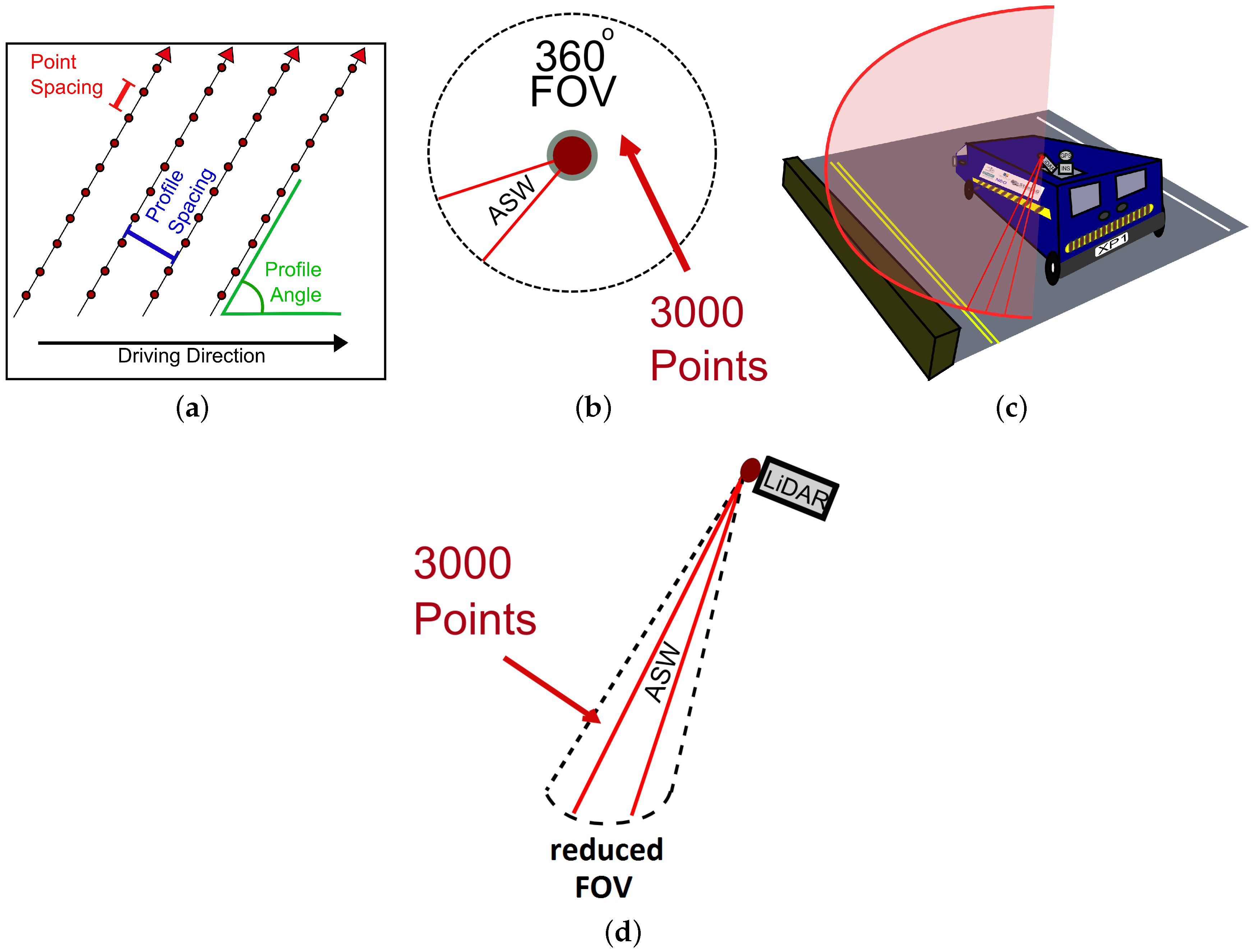
3.2. Enabling Use of Lower Specification Scanner through Field of View Manipulation

The Field of View (FOV) of a scanner is a user selectable setting. Full circle scanners (Figure 3b) must balance the mirror speed and the PRR as this dictates the minimum angular change between each laser pulse, termed the angular step width (ASW) or increment. However, the FOV can be set to limit a survey to a particular area around the MMS (Figure 3c) and by decreasing the FOV and maintaining the maximum effective measurement rate (EMR) it is possible to achieve a smaller ASW (Figure 3d). A smaller ASW will decrease point spacing in this area and therefore increase point density. Although the maximum measurement range for natural targets decreases as the EMR increases, (for example 75 m at 300 KHz EMR for the Riegl VQ-250) this will not influence performance for surveying roadside infrastructure as this is generally well within a 75 m range. In our Riegl VQ-250 full circle scanner, the angular stepwidth is a user-read parameter which can be varied depending on the FOV and the PRR. This is performed through the scanner interface by specifying a start and stop angle for the beam in the scanner coordinate system at which acquisition will start and stop. Laser pulses are subsequently limited to inside this angular portion of the 2D scan plane and this enables a greater concentration of pulses in a smaller area when the PRR is maintained. To achieve the lowest ASW specified in the manual, we are obliged to reduce the FOV because a 360${}^{°}$ FOV and an ASW of 0.018${}^{°}$ would not be compatible with the EMR limits of this scanner.

• Meas-set-prg (“300 kHz”)—sets the measurement programme for the scanner at 300 kHz
• Scn-set-Scan (20.0, 60.0, 0.013) specifies a 2D, 40${}^{°}$ scan at 300 kHz enabling a decreased increment of 0.013 degrees between each pulse increasing point density

It is important to note that the PRR and mirror frequency cannot be decreased/increased outside of the the specified operating range for that scanner. This is restricted by the hardware limitations and software interface. MIMIC is designed to demonstrate the potential for adjusting scanner hardware settings to optimise performance during particular surveys while adhering to realistic performance bounds.

A series of tests were designed to demonstrate the correlation between FOV, PRR and point spacing. These tests were carried out on a parallel vertical target of dimensions 2 m × 1 m for a 2D scanner operating a full-circle 360${}^{°}$ FOV. Figure 4 displays the profile spacing and point spacing for the scanner using a 360${}^{°}$ FOV. To demonstrate the benefit of reducing FOV on point spacing, the PRR was then tested in 50 kHz increments and the FOV was then decreased in 45${}^{°}$ increments for each PRR. The point density was calculated for the target after each decrease. The FOV was not decreased below 180${}^{°}$ for two reasons.

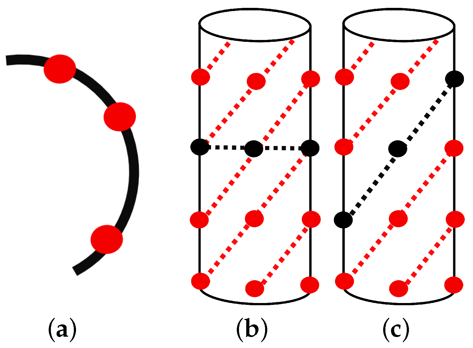
• Limiting the FOV could result in incomplete scan coverage of an area. In the example illustrated in Figure 3c the scanner is assigned a dual axis rotation and the FOV is limited to 180${}^{°}$. With this configuration, the road under the vehicle is not surveyed.
• A low FOV could also potentially decrease the ASW below the smallest selectable ASW for that piece of hardware. For example, the minimum quoted possible ASW for a Riegl VQ250 is 0.001${}^{°}$. This may become an issue at lower FOVs and for this reason 180${}^{°}$ is the cut-off for these tests.

A mirror speed ($M_f$) of 100 Hz was defined in these tests and a constant horizontal range to the target of 5 m was applied. Figure 4 illustrates the results for the FOV tests and the effect of decreasing FOV for increased point spacing. The impact of a higher FOV on point spacing is linear. For specific targets the point density can be increased if the area of interest in relation to the MMS is defined beforehand. If the Surveyor is certain that no extra features or redundancy from different scanner viewpoints is required, this is an optimal solution. Examples of potential targets could be road-side crash barriers, bollards, hedgerows or kerb-stones and by minimising the FOV, the area of interest can be surveyed with a higher point density than possible with the default operating settings.

4. Test Systems

MIMIC enables benchmarking of multiple scanner configurations in terms of their point density. Three MMSs were assessed in these tests, as illustrated in Figure 5. The hardware and configuration of these three theoretical MMS are described in this section. One system employs MIMIC to improve performance, and the second uses a scanner with a high PRR and the second with a high mirror speed. Scanner elevations were standardised for each system at the height of the scanner on the XP1, which is 3.1 m. This ensured that the results are dependent on the hardware configuration only and not influenced by the dimensions of the platform.

4.1. System 1—MIMIC+

The XP1 designed at the NCG is a single scanner system employing a single VQ-250. Incorporating another high specification scanner can be very costly and increases data throughput on the MMS and therefore MIMIC was used to identify optimum parameters for incorporating a lower specification scanner and maintaining a suitable point density. This system, entitled ‘MIMIC+’, incorporates a generic, limited FOV, low PRR laser profiler operating a rotating mirror.

Table 1. XP1+ Scanner Parameters.

System	Scanner	Hrot	VRot	${\mathit{M}}_{\mathit{f}}$	PRR	FOV	ASW
MIMIC+	Geom1	45	60	100 Hz	300 kHz	360${}^{°}$	0.12${}^{°}$
FOV1	135	60	75 Hz	27.075 kHz	180${}^{°}$	0.99${}^{°}$
PRR+	PRR1	45	45	100 Hz	300 kHz	360${}^{°}$	0.12${}^{°}$
PRR2	45	60	100 Hz	300 kHz	360${}^{°}$	0.12${}^{°}$
Mirror+	Mirror1	45	45	200 Hz	200 kHz	360°	0.36${}^{°}$
Mirror2	45	60	200 Hz	200 kHz	360${}^{°}$	0.36${}^{°}$

lists the relevant parameters of the two scanners on the MIMIC+. The PRR of the second scanner was only 9% that of the Riegl VQ250. This shortcoming was partially offset by the lower FOV of Scanner 2 which decreases the ASW. The two scanners were orientated and positioned in accordance with the recommended configuration identified in [34]. The 60${}^{°}$ vertical rotation identified in tests [34] was applied to both scanners to maximise point density. Horizontal scanner rotations of 45${}^{°}$ and 135${}^{°}$ were applied respectively.

4.2. System 2—PRR+

The PRR+ incorporates a second VQ-250 scanner but has retained the XP1’s 45${}^{°}$/45${}^{°}$ horizontal and vertical rotations scanner orientation, therefore not using the improved orientation calculated using MIMIC. This system is designed to replicate those MMSs that prioritise pulse repetition rate. The second scanner is negatively rotated to −45${}^{°}$/45${}^{°}$ as detailed in Table 1. The second scanner was offset by 1 m in the X axis, this standard offset is assigned to enable a comparison between the XP2 and the Mirror+.

4.3. System 3—Mirror+

The third system was designed to simulate a MMS that prioritises mirror frequency over PRR. These MMSs are capable of a higher mirror frequency PRR systems resulting in more scan lines but the lower PRR results in a reduced point spacing.

5. Benchmarking MMS Performance

The initial benchmarking tests assessed the performance of each system in terms of three key parameters: point density, profile spacing and point spacing. The target range and vehicle velocity was varied in these tests to facilitate a robust comparison of the three systems.

Table 2. Tests details and target information.

Test	Characteristic	Surface	Target	Dimensions	Variable
1	Point Density	2D	Planar	2 m × 1 m	Velocity
2	Profile Spacing	2D	Planar	2 m × 1 m	Velocity
3	Point Spacing	2D	Planar	2 m × 1 m	Range
4	Point Density	3D	Structure	2 m × 2 m	Velocity
5	Points Per Profile	3D	Cylinder	0.1 m × 2 m	Range

lists each of the point cloud characteristics that will be assessed for each system, the MMS operating parameters that will vary (velocity or range) and details of each target type, either 2D planar targets or 3D structures.

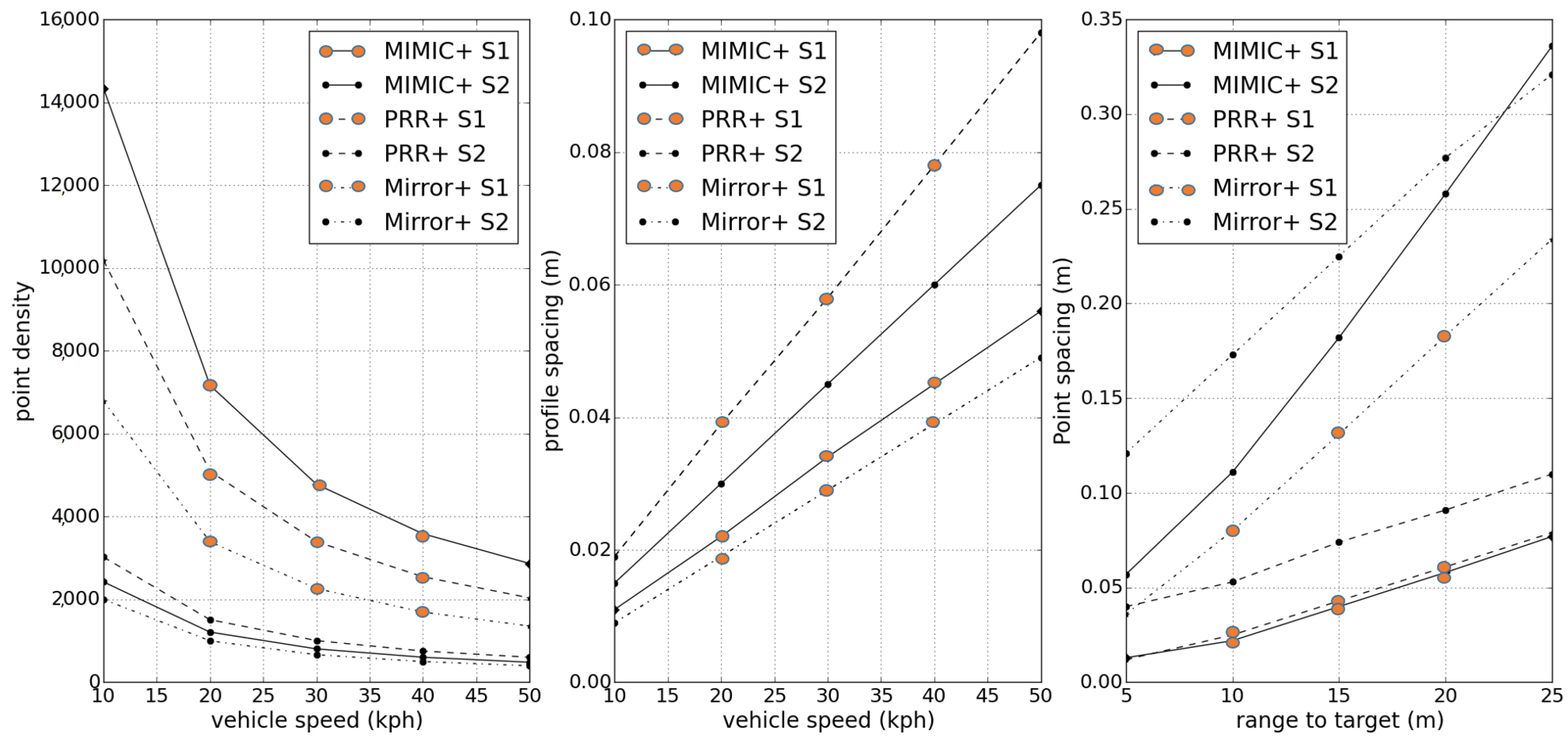
5.1. Test 1—2D Targets

Test 1 involved calculating the number of pulses striking a target at five vehicle velocities ranging from 10 km/h to 50 km/h in 10 km/h increments. In Figure 6 these results are plotted as a function of velocity for all three MMSs. These tests highlight the link between PRR and point density, as each of the higher PRR scanners on both MIMIC+ and PRR+ captured the highest number of points. Importantly, MIMIC+, developed using GAD, is capable of a combined higher point density than the other systems operating high-grade second scanners. This demonstrates the positive effect of implementing the recommended scanner configuration identified in [34].

For instance, at 10 km/h, Scanner 1 on board the MIMIC+ is capable of capturing 4155 points more than the same scanner on the PRR+. Applying the recommended configuration to Scanner 2 has also improved its performance. By eliminating the traditional scanner offset, limiting the FOV and introducing the recommended 60${}^{°}$ vertical scanner rotation, its performance is comparable (captured only 368 points less at 10 km/h) with the higher specification Scanner 2 the PRR+ system, and it outperformed (319 more pulses striking the target at 10 km/h) Scanner 2 on Mirror+. GAD has enabled MIMIC+ to achieve a higher point density than both of the other MMS.

5.2. Small Features

The tests in the previous section demonstrated that GAD can positively influence point density. However, for small targets, such as road markings, pot-holes or Cats’ eyes, profile spacing and point spacing are the key characteristics of the point cloud when determining a suitable resolution. Point spacing is influenced by range to target, PRR and the scanner orientation, whereas profile spacing is influenced by vehicle velocity, mirror speed and scanner orientation. These are key parameters in identifying which MMS configurations can potentially miss survey features due to unsuitable profile spacing or point spacing.

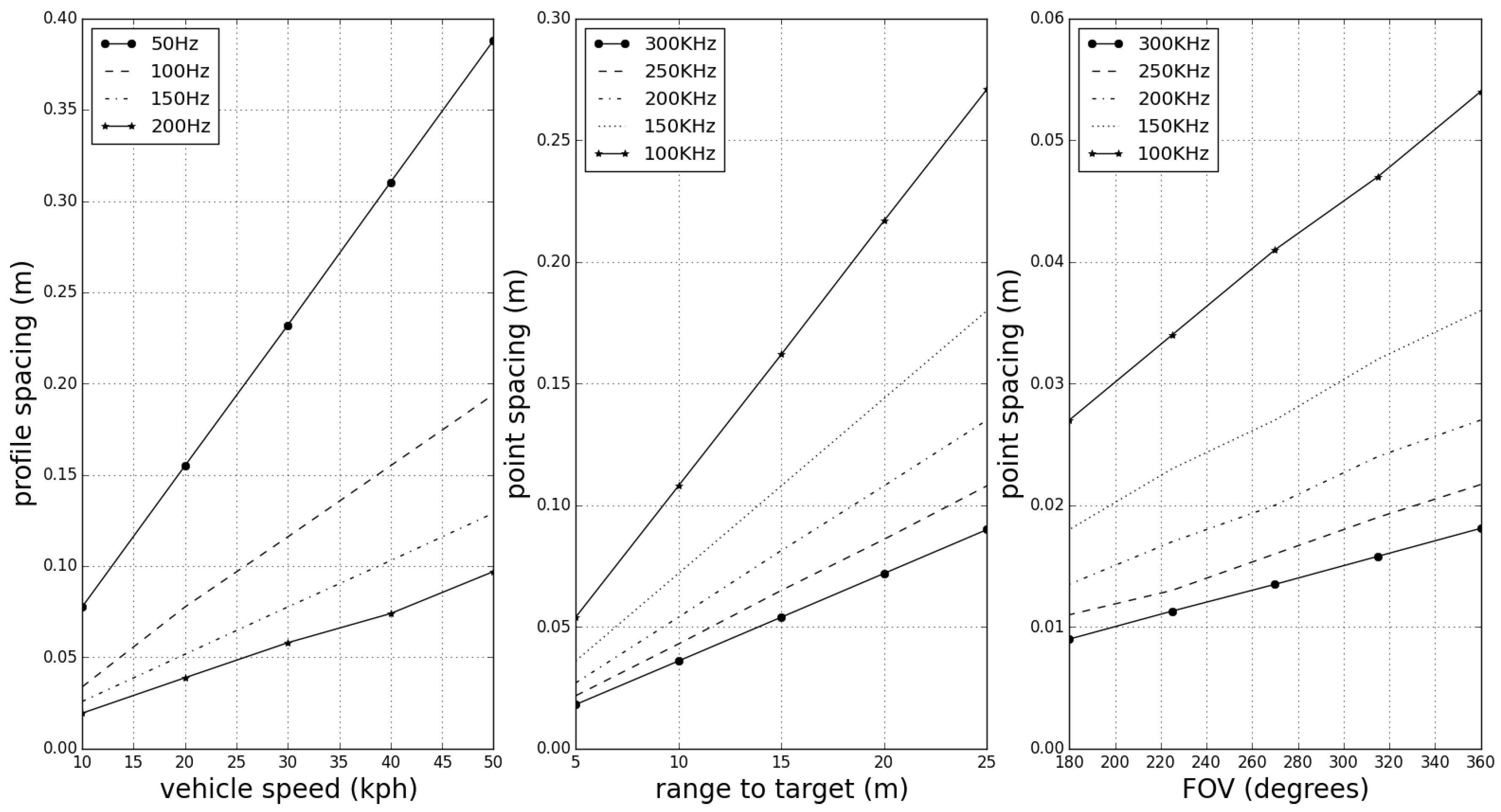
5.2.1. Test 2—Profile Spacing

Test 2 calculated profile spacing on a parallel vertical target. These results are detailed in Figure 6 at five vehicle velocities ranging from 10 km/h to 50 km/h in 10 km/h increments. MIMIC+ incorporates two different scanners and therefore the profile spacing is different for each and for this reason, both scanners are plotted in this figure. Because Scanner 1 and Scanner 2 on PRR+ and Mirror+ are identical, profile spacing does not differ on a parallel target and therefore only one scanner is plotted.

These tests demonstrate the impact that the higher $M_f$ has on profile spacing as the Mirror+ is capable of a smaller profile spacing than the other systems. At 10 km/h the PRR+ profile spacing of 0.027 m is almost twice as large as the profile spacing of the Mirror+ MMS which is 0.014 m. The profile spacing of the low-specification, Scanner 2 on MIMIC+ is not comparable with the second scanners on the other two systems, for example, at 10 km/h the profile spacing of 0.037 m for Scanner 2 on MIMIC+ is almost three times as large as that of the Mirror+. The Mirror+ profile spacing of 0.069 m at 50 km/h is similar to the 0.074 m profile spacing of the Scanner 2 on MIMIC+ at 20 km/h, however, GAD has enabled the 75 Hz Scanner 2 on MIMIC+ to minimise the profile spacing on the target and outperform both of the 100 Hz Scanners on the PRR+ MMS. In this case, GAD has demonstrated that changing the angle at which the scan disk interacts with the target can provide similar benefits to scanners capable of surveying with a higher mirror speed.

5.2.2. Test 3—Point Spacing

Point spacing was then calculated for each scanner on a parallel vertical target at different target ranges. As point spacing is not influenced by vehicle velocity, a constant velocity of 50 km/h was applied. Figure 6 lists the results from Test 3. In each test, the scanners with the highest PRR have the lowest point spacing. At all target ranges, the distance between subsequent LiDAR points captured by these scanners is over twice as low (43%) as the point spacing of the scanners on the Mirror+ MMS. Scanner 2 on MIMIC+ exhibits a higher point spacing in these tests because of its low PRR. At a range of 25 m, this scanner is exhibiting a point spacing that is over four times (419%) larger than the point spacing of Scanner 2 on PRR+. These results reinforce the significance in selecting the correct scanner configuration for increasing point density. Because of the application of GAD on MIMIC+, Scanner 2 produces comparable point density with Mirror+ and PRR+ scanners in the earlier tests on larger targets. However, these results demonstrate that this scanner is not suitable for surveying narrow targets at long ranges. For instance, for a target such as a circular road sign of radius 0.5 m at a 10 m horizontal range, a point spacing of 0.25 m would return an insufficient number of points to distinguish that object in the point cloud. For this target, it would result in two and possibly only one pulse striking the target per mirror rotation. In this scenario, Mirror+ has outperformed MIMIC+ with approximately five to six points on each scan profile whereas the PRR+ MMS performed best with over ten pulses striking the target per mirror rotation.

5.3. Angled Targets

The preceding tests dealt with parallel, planar targets. However, because the majority of roadside infrastructure are angled targets or have multiple faces, in this section, benchmarking tests are conducted to examine the performance of each MMS configuration for multi-faced targets, calculating point density on the angled surfaces of two multi-faced structures. The first structure was represented by three large vertical planes and the second structure, a cylinder, was represented by three narrow vertical planes.

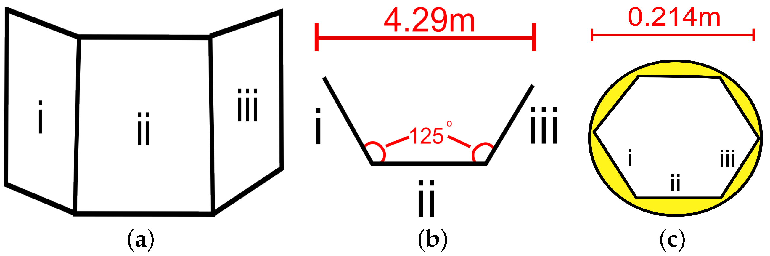
5.3.1. Test 4—Structures

The structure used in Test 4 was composed of three planar targets, one parallel to the road and two angled away from the road (Figure 7a). The top-down view in Figure 7b displays the angular rotation for each face of the target. A 125${}^{°}$ rotation corresponds to a 55${}^{°}$ rotation towards and away from the target for the two faces respectively. This target rotation was chosen to ensure that the scan plane resulting from the horizontal scanner rotation of Scanner 1 on each of the MMSs does not intersect with the third plane of the target, and therefore the coverage of Face (iii) depends on Scanner 2 only, a key reason for including a second scanner on a MMS. Similarly, Face (i) is not visible to Scanner 2. Face (ii), parallel to the road, was the only face that exhibited an overlap from both Scanner 1 and Scanner 2.

The point density for the three target faces are illustrated in Figure 8a.

• Face (i): The high PRR scanners display the highest point density on each face, however Scanner 1 on MIMIC+ is capable of capturing 11% more points than the same scanner on PRR+ because of its application of GAD. The high PRR scanners are each capable of over twice the number of points than the Mirror+ scanners.
• Face (ii): For each MMS, the point density is higher for this face of the target because it is visible to both scanners and it also has a lower range to target. GAD has enabled MIMIC+ to once again outperform the other two systems as it is capable of returning 37% more points than the higher specification PRR+ MMS for Face (ii).
• Face (iii): This target face is only visible to Scanner 2 on each of the MMSs. The low point density is due to the negative horizontal scanner rotation of Scanner 2 on the PRR+ and the Mirror+ and the scanner offset. In these tests, Scanner 2 on the PRR+ exhibits a higher point density than Scanner 2 on the other systems because of the higher PRR, returning over three times (327%) the point density of the Scanner 2 on the MIMIC+ MMS. Scanner 2 on Mirror+ also exhibits a higher point density than Scanner 2 on MIMIC+, returning 89% more points. Despite the decreased range to target arising from the recommended scanner position on MIMIC+, Scanner 2 on this MMS has underperformed in these tests in relation to Scanner 2 on the Mirror+.

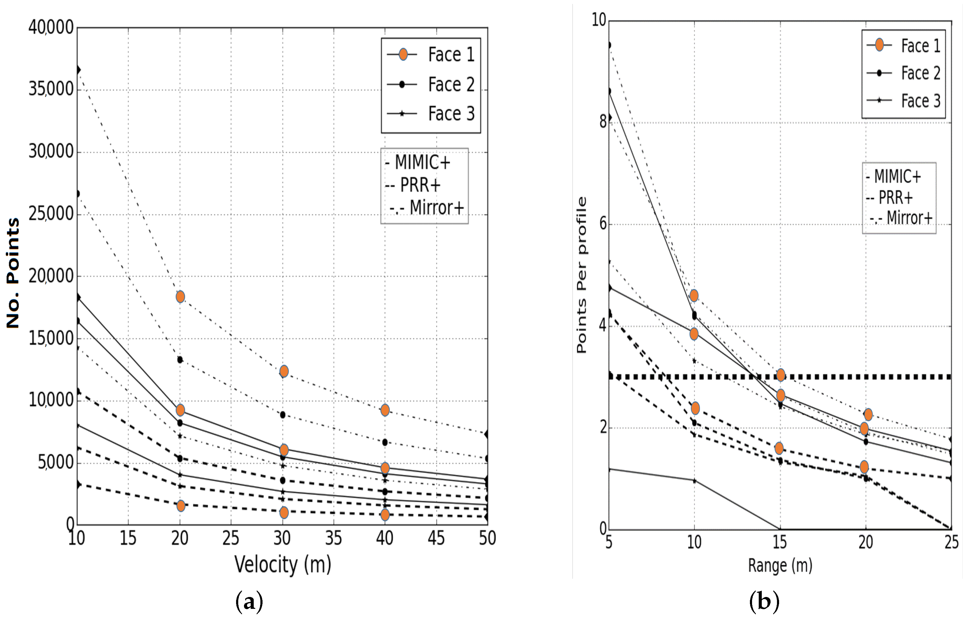
5.3.2. Test 5—Cylinders

The angled target that is used in Test 5 is also composed of three planar faces, one facing the road and two angled away from the road. This is a hexagonal approximation of a cylindrical target. Figure 7c illustrates the cylinder that is used in the benchmarking tests. The cylinder is 0.214 m in diameter, and each face of the cylinder is 0.1 m wide and 2 m high, approximating the cylindrical support of a traffic sign-post. In the previous tests, a high number of points was an indicator of good performance, however, for narrow features, a high number of points striking the target does not necessarily define a target if these points result from a large number of profiles intersecting the target. A high number of profiles implies a lower number of points per profile ($P_{\mathrm{pp}}$).

The minimum number of points required to define a fixed radius curve is three, as illustrated in Figure 9a. Figure 9b illustrates a cylinder with the three required points marked on it. These three points are at the same elevation on the target, however scanner orientations alter this scenario. Figure 9c illustrates a scan profile crossing one face of a cylindrical target with 3 $P_{\mathrm{pp}}$. In this scenario, the 3 $P_{\mathrm{pp}}$ are at different elevations. However, it is reasonable to assume that for a narrow target, the 3 $P_{\mathrm{pp}}$ do not deviate significantly in elevation. For example, a profile angle of 45${}^{°}$ results in a height deviation between the first and third point of only 0.085 m for a target face 0.1 m wide. It was also reasonable to assume that a change in radius of the cylinder is unlikely over that short distance. Therefore, specifying that a minimum of 3 $P_{\mathrm{pp}}$ are required from angled scan profiles on cylindrical targets is justifiable. These tests demonstrate that for varying target parameters and MMS configurations, only a number of the scan profiles meet this criteria. Figure 8b plots point density as a function of range for a narrow vertical target. This image also highlights the 3 $P_{\mathrm{pp}}$ cut-off. These results highlighted a number of issues:

• Firstly, except for one instance with the PRR+ on Face (i), none of the MMSs used in these benchmarking tests can return the required number of $P_{\mathrm{pp}}$ on a cylindrical target at 15 m horizontal range.
• Performance in terms of $P_{\mathrm{pp}}$ drops significantly between 5 m and 10 m horizontal range for narrow vertical targets. The number of $P_{\mathrm{pp}}$ approximately halves as the range doubles. The PRR+ MMS returned the most points for each cylinder face in these tests, but only returns a maximum of 5 $P_{\mathrm{pp}}$ at 10 m range.
• At the shortest measurement range, 5 m, the Mirror+ MMS returns 4 $P_{\mathrm{pp}}$, whereas the PRR+ returns 8. Eight $P_{\mathrm{pp}}$ potentially provide a better definition of the object in the point cloud.
• Scanner 2 on MIMIC+ fails these tests as it was not capable of capturing the three points on the scan profile for Face (iii), however Scanner 1 has returned a high number of points on the two other faces and therefore this is not essential.

6. Conclusions

This paper presented three potential methods for increasing MMS performance using Geometry Aided Design, a methodology developed at Maynooth University. Utilising the Y axis of the MMS allowed the second scanner to be positioned in a location with dual-benefits, it can eliminate data shadows but also provide a higher point spacing and point density. GAD also demonstrated a methodology whereby a lower specification 2D laser profiler with a low pulse repetition rate and mirror frequency can compare with higher specification hardware by utilising a higher vertical orientation and also limiting the FOV. As the majority of MMS surveys require the MMS to travel in both directions due to potential obstructions, data shadows etc., concentrating the scanners on one side of the MMS is a practical solution and results in an increased point density. These tests benchmarked three hypothetical MMS and demonstrated how MIMIC and GAD can be used to improve MMS performance.

References

1. Puente, I.; González-Jorge, H.; Martínez-Sánchez, J.; Arias, P. Review of mobile mapping and surveying technologies. Measurement 2013, 46, 2127–2145. [Google Scholar] [CrossRef]
2. Graham, L. Mobile mapping systems overview. Photogramm. Eng. Remote Sens. 2010, 76, 222–228. [Google Scholar]
3. McElhinney, C.; Kumar, P.; Cahalane, C.; McCarthy, T. Initial results from European Road Safety Inspection (EURSI) mobile mapping project. In Proceedings of the ISPRS Commission V Technical Symposium, Newcastle, UK, 21–24 June 2010.
4. Becker, S.; Haala, N. Grammar supported facade reconstruction from mobile LiDAR mapping. In Proceedings of the ISPRS CMRT09, Paris, France, 3–4 September 2009; pp. 229–234.
5. Hammoudi, K.; Dornaika, F.; Paparoditis, N. Extracting building footprints from 3D point clouds using terrestrial laser scanning at street level. In Proceedings of the ISPRS CMRT09, Paris, France, 3–4 September 2009; pp. 65–70.
6. Kumar, P.; McCarthy, T.; McElhinney, C. Automated road extraction from terrestrial based mobile laser scanning system using the GVF snake model. In Proceedings of the European Laser Mapping Forum—‘ELMF 2010’, The Hague, The Netherlands, 30 November–1 December 2010.
7. Kumar, P.; McElhinney, C.; McCarthy, T. Utilizing terrestrial mobile laser scanning data attributes for road edge extraction with the GVF snake model. In Proceedings of the 7th International Symposium on Mobile Mapping Technology (MMT’11), Cracow, Poland, 13–16 June 2011.
8. Pu, S.; Vosselman, G. Extracting windows from terrestrial laser scanning. In Proceedings of the ISPRS Workshop on Laser Scanning 2007 and SilviLaser 2007, Espoo, Finland, 12–14 September 2007; Volume 36, pp. 320–325.
9. Pu, S.; Rutzinger, M.; Vosselman, G.; Elberink, S.O. Recognizing basic structures from mobile laser scanning data for road inventory studies. ISPRS J. Photogramm. Remote Sens. 2011, 66, S28–S39. [Google Scholar] [CrossRef]
10. Brenner, C. Global localization of vehicles using local pole patterns. In Pattern Recognition; Denzler, J., Notni, G., Süße, H., Eds.; Lecture Notes in Computer Science; Springer: Berlin/Heidelberg, Germany, 2009; Volume 5748, pp. 61–70. [Google Scholar]
11. Kukko, A.; Jaakkola, A.; Lehtomaki, M.; Kaartinen, H.; Chen, Y. Mobile mapping system and computing methods for modelling of road environment. In Proceedings of the 2009 Joint Urban Remote Sensing Event, Shanghai, China, 20–22 May 2009.
12. Lehtomäki, M.; Jaakkola, A.; Hyyppä, J.; Kukko, A.; Kaartinen, H. Detection of vertical pole-like objects in a road environment using vehicle-based laser scanning data. Remote Sens. 2010, 2, 641–664. [Google Scholar] [CrossRef]
13. Kaartinen, H.; Hyyppä, J.; Gülch, E.; Vosselman, G.; Hyyppä, H.; Matikainen, L.; Hofmann, A.D.; Mäder, U.; Persson, A. Accuracy of 3D City Models: EuroSDR comparison. In Proceedings of the International Archives of Photogrammetry, Remote Sensing and Spatial Information Sciences, Enschede, The Netherlands, 12–14 September 2005; pp. 227–232.
14. Yoo, H.; Goulette, F.; Senpauroca, J.; Lepere, G. Simulation based comparative analysis for the design of laser terresttrial mobile mapping. In Proceedings of the 6th International Symposium on Mobile Mapping Technology, Sao Paulo, Brazil, 21–24 July 2009; pp. 839–854.
15. Bolzon, G.; Caroti, G.; Piemonte, A. Accuracy check of road’s cross slope evaluation using MMS vehicle. In Proceedings of the 5th International Symposium on Mobil Mapping Technology, Padua, Italy, 28–31 May 2007; pp. 127–132.
16. Florida Department of Transport. Terrestrial Mobile LiDAR Surveying and Mapping Guidelines; Florida Department of Transport: Tallahassee, FL, USA, 2012.
17. Yen, K.S.; Ravani, B.; Lasky, T.A. LiDAR for Data Efficiency; University of California: Oakland, CA, USA, 2011. [Google Scholar]
18. Olsen, M.J.; Roe, G.V.; Glennie, C.; Persi, F.; Reedy, M.; Hurwitz, D.; Williams, K.; Tuss, H.; Squellati, A.; Knodler, M. NCHRP 15–44 Guidelines for the Use of Mobile LiDAR in Transportation Applications; NCHRP: Washington, DC, USA, 2013. [Google Scholar]
19. Trimble. Trimble MX8 Mobile Mapping System; Trimble: Sunnyvale, CA, USA, 2010. [Google Scholar]
20. Optech. Optech Lynx M1 and V200 System Specifications; Optech: Vaughan, ON, Canada, 2012. [Google Scholar]
21. RIEGL. Dual Scanner Data Sheet Riegl VMX-450; RIEGL: Horn, Austria, 2016. [Google Scholar]
22. Laser Mapping. StreetMapper Brochure; Technical Report; 3D Laser Mapping: Nottingham, UK, 2012. [Google Scholar]
23. Kukko, A.; Andrei, C.; Salminen, V.; Kaartinen, H.; Chen, Y.; Rönnholm, P.; Hyyppä, H.; Hyyppä, J.; Chen, R.; Haggrén, H.; et al. Road environment mapping system of the finnish geodetic institute-FGI roamer. In Proceedings of the ISPRS Workshop on Laser Scanning 2007 and SilviLaser 2007, Espoo, Finland, 12–14 September 2007; pp. 241–247.
24. Hesse, C.; Kutterer, H. A mobile mapping system using kinematic terrestrial laser scanning (KTLS) for image acquisition. In Proceedings of the 8th Conference on Optical 3-D Measurement Techniques, Zurich, Switzerland, 9–12 July 2007; pp. 134–141.
25. Lohani, B.; Mishra, R. Generating LiDAR data in laboratory: LiDAR simulator. In Proceedings of the ISPRS Workshop on Laser Scanning 2007 and SilviLaser 2007, Espoo, Finland, 12–14 September 2007; Volume 52, pp. 12–14.
26. Kukko, A.; Hyyppä, J. Small-footprint laser scanning simulator for system validation, error assessment and algorithm development. Photogramm. Eng. Remote Sens. 2009, 75, 1177–1189. [Google Scholar] [CrossRef]
27. Kaartinen, H.; Hyyppä, J.; Kukko, A.; Jaakkola, A.; Hyyppä, H. Benchmarking the performance of mobile laser scanning systems using a permanent test field. Sensors 2012, 12, 12814–12835. [Google Scholar] [CrossRef]
28. Cahalane, C.; McCarthy, T.; McElhinney, C. MIMIC: Mobile mapping point density calculator. In Proceedings of the 3rd International Conference on Computing for Geospatial Research and Applications, Reston, VA, USA, 1–3 July 2012.
29. Cahalane, C.; McCarthy, T.; McElhinney, C. Mobile mapping system performance: An initial investigation into the effect of vehicle speed on laser scan lines. In Proceedings of the Remote Sensing & Photogrammety Society Annual Conference—‘From the Sea-Bed to the Cloudtops’, Cork, Ireland, 1–3 September 2010.
30. Cahalane, C.; McElhinney, C.; McCarthy, T. Mobile mapping system performance: An analysis of the effect of laser scanner configuration and vehicle velocity on scan profiles. In Proceedings of the European laser Mapping Forum—‘ELMF 2010’, The Hague, The Netherlands, 30–31 November 2010.
31. Cahalane, C.; McElhinney, C.; McCarthy, T. Calculating the effect of dual-axis scanner rotations and surface orientation on scan profiles. In Proceedings of the 7th International Symposium on Mobile Mapping Technology (MMT’11), Cracow, Poland, 13–16 June 2011.
32. Cahalane, C.; McElhinney, C.; Lewis, P.; McCarthy, T. Calculation of target-specific point distribution for 2D mobile laser scanners. Sensors 2014, 14, 9471–9488. [Google Scholar] [CrossRef] [PubMed]
33. Cahalane, C.; McElhinney, C.; Lewis, P.; McCarthy, T. MIMIC: An innovative methodology for determining mobile laser scanning system point density. Remote Sens. 2014, 6, 7857–7877. [Google Scholar]
34. Cahalane, C.; Lewis, P.; McElhinney, C.; McCarthy, T. Optimising mobile mapping system laser scanner orientation. ISPRS Int. J. Geo-Inf. 2015, 4, 302–319. [Google Scholar] [CrossRef]
35. Shepard, D. A two-dimensional interpolation function for irregularly-spaced data. In Proceedings of the 23rd National Conference ACM, Las Vegas, NV, USA, 27–29 August 1968; pp. 517–524.
Figure 1. Understanding the impact of changes in scanner orientation (a) horizontal rotations of the scanner increase the distance to roadside infrastructure (b) horizontal scanner angle—distance to targets on both sides of the MMS is also increased, thereby reducing point density on both sides of the MMS (c) vertical rotations of the scanner increase the distance to the road surface, also reducing point density. The blue marker is the closest point to the scanner on the road surface and will exhibit the highest point density.
Infrastructures 01 00005 g001
Figure 2. Enabling system performance improvements (a) horizontal scanner position—scanners 1, 2, 3 and 4 situated on both the X and Y axes (b) target orientations used in the tests (c) results from the performance tests.
Infrastructures 01 00005 g002
Figure 3. Changing scanner Field of View (FOV) to improve point spacing (a) point cloud characteristics for a mobile mapping system survey using a 2D scanner (b) a full-circle FOV will distribute the max number of pulses per mirror rotation around the full 360 ° (c) decreasing FOV enables a MMS to focus laser pulses on one side of the vehicle (d) limiting the FOV then allows the max number of pulses per mirror rotation to be distributed throughout this reduced FOV, decreasing point spacing.
Infrastructures 01 00005 g003
Figure 4. The effect of changing scanner settings such as Pulse Repetition Rate (PRR), mirror frequency and decreasing the scanner FOV on the coverage of the environment.
Infrastructures 01 00005 g004
Figure 5. Mobile Mapping Systems (MMS) in benchmarking tests (a) MIMIC+ Scanner Locations (b) PRR+ Scanning Locations (c) Mirror+ locations.
Infrastructures 01 00005 g005
Figure 6. Benchmarking results for each dual-scanner MMS in terms of point density, profile spacing and point spacing related to vehicle velocity and range to target.
Infrastructures 01 00005 g006
Figure 7. Target representing a structure (a) front view (b) top-down view (c) planar faces for the cylindrical target.
Infrastructures 01 00005 g007
Figure 8. Mobile Mapping System performance on structures (a) point density on a multifaced structure (b) number of points per profile on a cylinder with three points per profile threshold defined as the minimum to describe a curve.
Infrastructures 01 00005 g008
Figure 9. Quantifying the number of P pp required. (a) Defining a fixed radius curve using three points (b) three points at the same elevation (c) three points at different elevations.
Infrastructures 01 00005 g009