Development of an Eco-Cruise Control System Based on Digital Topographical Data

Abstract

Rapid growth in economies and a sharp increase in the present quantity of vehicles have contributed to congested cities, traffic accidents, energy crises and air pollution, which not only cause serious economic damage but also affect human life and safety. According to the Kyoto Protocol international standards and consensus, the trend in the automotive industry is to develop more ecological vehicles in order to reduce fuel consumption and air pollution. Recently, a number of modern premium cars have been equipped with advanced driver assistance systems (ADAS), especially an adaptive cruise control (ACC) system, which was found to be one of the most widely and successful ADAS systems to date. However, the road topography on highways affects fuel consumption of vehicles. Rapid acceleration, rapid deceleration, and unreasonable gear use can all result in increasing fuel consumption. Therefore, an eco-cruise control (ECC) system on roads with up-down slopes is critical for improving vehicle fuel economy in coordination with the Global Positioning System (GPS) and Geographic Information System (GIS). This proposed approach combines the road elevation profile of digital road maps with nonlinear optimal predictive control (NOPC) algorithms to handle the vehicle velocity control; it is aimed at providing the most economical speed according to road grade. The developed algorithms not only provide ecological driving guidance for the driver, but also contribute to driving safety. Finally, extensive simulations demonstrate that the proposed controller can significantly reduce fuel consumption of a vehicle while ensuring driving comfort and safety.

1. Introduction

Spurred on by the oil crisis and global warming as well as considerations about traffic congestion and aging societies, most countries have started to promote renewable energy and energy efficiency in recent years, especially focusing on energy conservation and environmental protection. According to the Energy Technology Perspective 2014 [1] published by the International Energy Agency (IEA), the transport sector is responsible for around 19% of total energy consumption. The report also indicates that the fuel efficiency of vehicles should be increased once to offset the transportation needs of doubling the impact when increasing warming by two degrees; therefore, energy efficiency and low-carbon transport systems have become priority for transport policy in the future. In addition, the Organization of the Petroleum Exporting Countries (OPEC) has increased oil production causing continuous decrease in crude oil prices to avoid losing their advantage. Although there are currently sufficient oil reserves, these will be exhausted eventually. In order to slow down oil consumption and the greenhouse effect, energy-saving technology and alternative energy has become the focus of research and development in the automotive industry, such as electric vehicles, hybrid/Plug-in hybrid vehicles, fuel cell vehicles, natural gas vehicles and other types of vehicles. Plenty of new fuel cell vehicles were launched at the 2015 Tokyo Motor Show, such as Lexus LS-FCV [2], Toyota Mirai [3], BMW Hydrogen 7 [4], and Honda FCX Clarity [5]; however, all of these vehicles are concept cars and it will still be a long journey to replace the normal car. In recent years, each automotive company mainly focuses on developing safer, more environmentally friendly, more autonomous, more intelligent driving assistance systems, especially new types and renewable of energy such as hydrogen and electric power for vehicles. However, they did not consider an ecological driving assistance system to improve your car's fuel economy when vehicle on roads with up-down slopes. Therefore, this paper will design an eco-cruise control system based on digital topographical data and the proposed nonlinear optimal predictive control algorithm for eco-driving.

According to domestic and international studies, eco-driving can reduce fuel consumption and reduce the accident rate. Nowadays, Japanese companies such as Honda, Toyota, Nissan, the American vehicle company Ford, and European vehicle makes such as BMW, and Volkswagen, and other automakers have started to equip their vehicles with eco-driving assistance systems, such as the Honda Insight built-in energy-saving ECO Assist system [6], that helps drivers develop driving habits that enhance fuel efficiency and generate driving pleasure by displaying fuel efficiency in real time and providing Eco Sore process with ECO automatic energy saving mode, a Guidance energy saving guiding function, and a scoring energy saving scoring function. BMW have an ecological indicator that shows “ECO PRO” mode [7], which minimizes fuel consumption by optimizing accelerator pedal and transmission shift parameters and settings, as well as heating/air conditioning strategy. Meanwhile, the whole fuel reduction process can be displayed on the screen. However, the technologies mentioned above basically need to be activated by users before entering the energy-saving mode, and mainly play the role of assisting drivers with fuel saving driving behaviors. In addition, current eco-driving assistance systems are mainly applied in small passenger vehicles; however, it is more important for heavy vehicles to save energy. According to energy bureau statistics [8], although heavy vehicles only represent 1.1% of total vehicles domestically, they represent 27.7% of energy consumption. Moreover, driving heavy vehicles rather than small passenger vehicles using unreasonable acceleration, deceleration or incorrect shift switch on mountain roads, or up and down roads, results in more fuel consumption and environmental pollution.

In the past decade, lot of significant researches on ecological driving have emerged [9,10,11,12,13,14,15,16,17,18,19]. The central issue of most published literature is to find a control strategy to enhance the driving safety and fuel efficiency of a vehicle, such as sliding mode control [14], optimal control [10,12,15,16], and model predictive control (MPC) [11,13,17]. MPC is a model based process control technique that has received a great deal of attention for vehicle control applications, because its formulation is best suited to online optimizations, and for dealing with constraints in controlling highly complex dynamic systems. However, some of the above designed strategies are not suited to real-time implementation as they require extra knowledge of the driver’s full driving behavior before they can be effective. Wang et al. [12] took advantage of the rolling horizon optimal control strategy to design an ecological driver assistance system for a platoon of vehicles in the ring-road scenario. The ecological driving strategy results in a lower spatial CO₂ emission rate than the efficient-driving strategy, both in free traffic and in moderately congested conditions. However, the effect of road terrain, only demonstrated on the flat urban environment, is not considered. In addition, a novel ecological driving systems based on model predictive control (MPC) theory for traveling on roads with up-down slopes has been proposed [10]. The simulation results shown that the MPC controllers can improve fuel efficiency significantly. However, the transfer function between actuator and the vehicle propulsion system is not considered in the system model. Luo et al. [15] also employed a MPC framework for designing adaptive cruise control (ACC) systems, which was given to guarantee not only car-following performance, and better fuel economy, but also improve comfort for passengers. In addition, a more realistic approach [16] to utilized information on traffic signs and road gradients is presented for eco-driving. However, it may not be applicable with immediately perceived road elevation information; in addition, it needs to know all of the traffic sign information on the planned route before the trip. Unlike previous publications, the main contribution of this paper presents an efficient and simple ECC system by using rolling horizon dynamic programming and taking a penalty function as the soft constraints for the design of a nonlinear optimal predictive controller for ecological driving on hilly roads. The ECC system can significantly improve the total fuel efficiency of driving, while also guaranteeing the driving safety and comfort. Additionally, the actuator and the vehicle propulsion system can be modeled as a time delay in cascade with a first order and a lag, so that simulation results are closer to the actual dynamic situation.

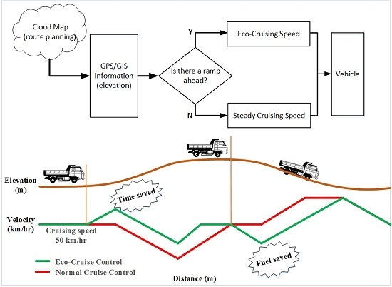
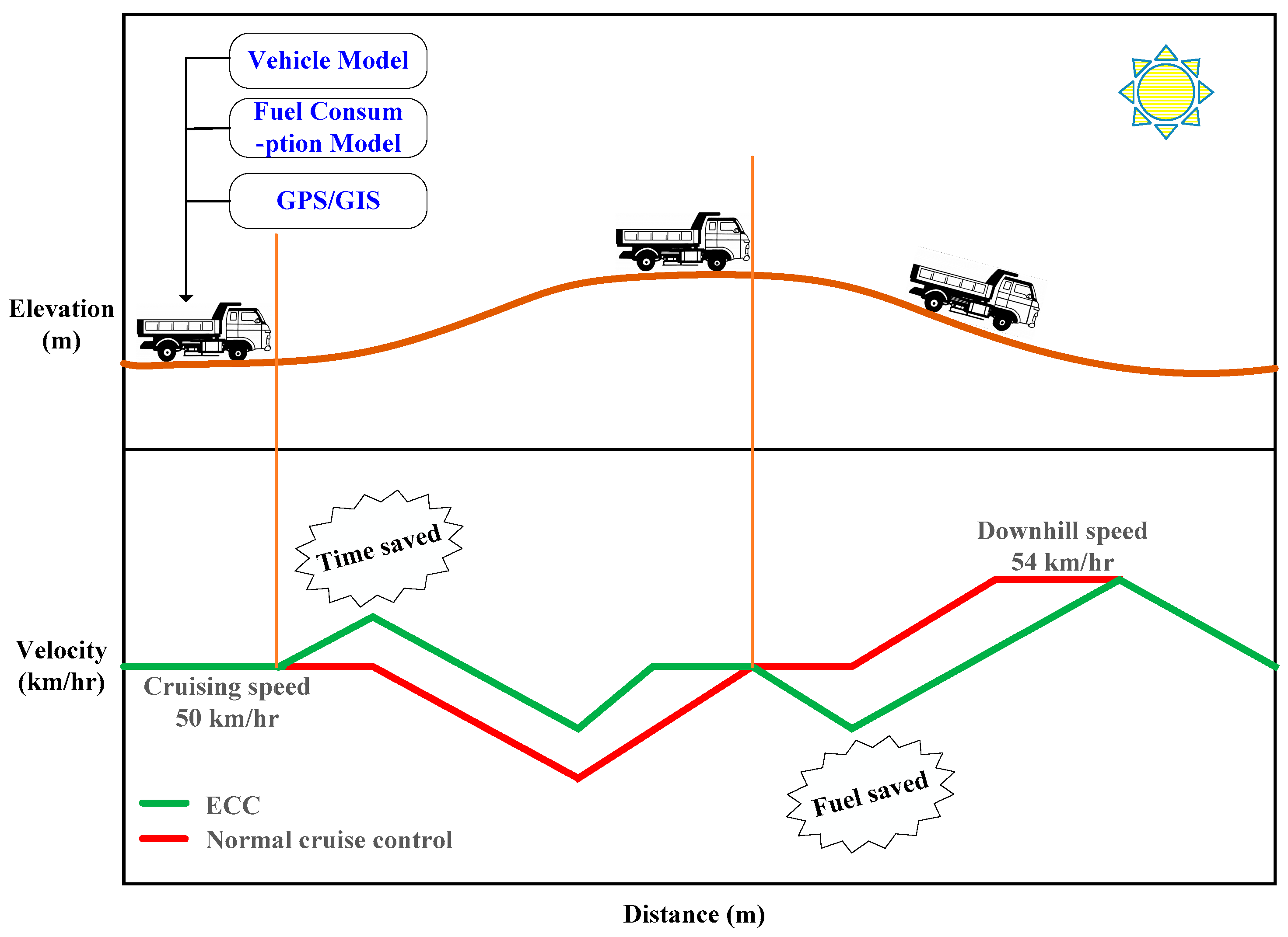
A comparison diagram of cruising speed in normal cruise control system and eco-cruise control system on the road with up-down slopes is shown in Figure 1. The proposed ECC system utilizes the vehicle dynamics model, fuel consumption model and information on road gradients from GPS/GIS. In Figure 1, the red line represents the testing vehicle speed using the traditional cruise control strategy; the green line represents the testing vehicle speed using our proposed eco-cruise control strategy, respectively.

The main purpose of normal cruise control is to maintain a set cruising speed in all free driving conditions. Although normal cruise control strategy is convenient for the driver, it often leads to high fuel consumption and driver discomfort on hill roads. The vehicle will use a low gear, allowing the engine to operate at a higher RPM, to avoid losing speed when climbing a hill. In addition, the vehicle may be subject to unwanted braking to prevent unnecessary acceleration when driving downhill. In view of this, we know that excessive hard braking and over-accelerating behavior means a waste of fuel. Therefore, an eco-cruise control system based on digital topographical information and GPS is proposed. Thus, the position of the vehicle and altitude data of the road ahead can be determined, and then they can be used to calculate the most fuel-efficient speed profile on the planned route. Knowing the route, an eco-cruise controller for the vehicle will increase some extra speed before entering a hill. The vehicle speed is raised slightly the set cruising speed (normal cruising speed) when approaching an ascent, as shown in Figure 1. Moreover, before the start of a descent, the vehicle can ease off the throttle shortly to allow gravity to help the vehicle to slow down, with the help of momentum and weight, and ease down the hill. This strategy can save the most fuel. Consequently, an ecological driving system using the nonlinear optimal predictive control strategy is proposed in this paper. Based on the topographical information, GPS data, vehicle dynamic model, and fuel consumption model, a nonlinear optimal predictive control algorithm is implemented to generate appropriate control inputs (throttle and breaking) required for ecological driving on hilly roads. Not only does the proposed approach increases the fuel economy for ecological driving, which means avoiding frequent acceleration and deceleration behavior, but the resulting feedback control law also guarantees asymptotic stability for eco-cruise controller design. Finally, effectiveness of the proposed NOPC strategy is demonstrated by extensive numerical verifications of the proposed eco-cruise control system.

2. Materials and Methods

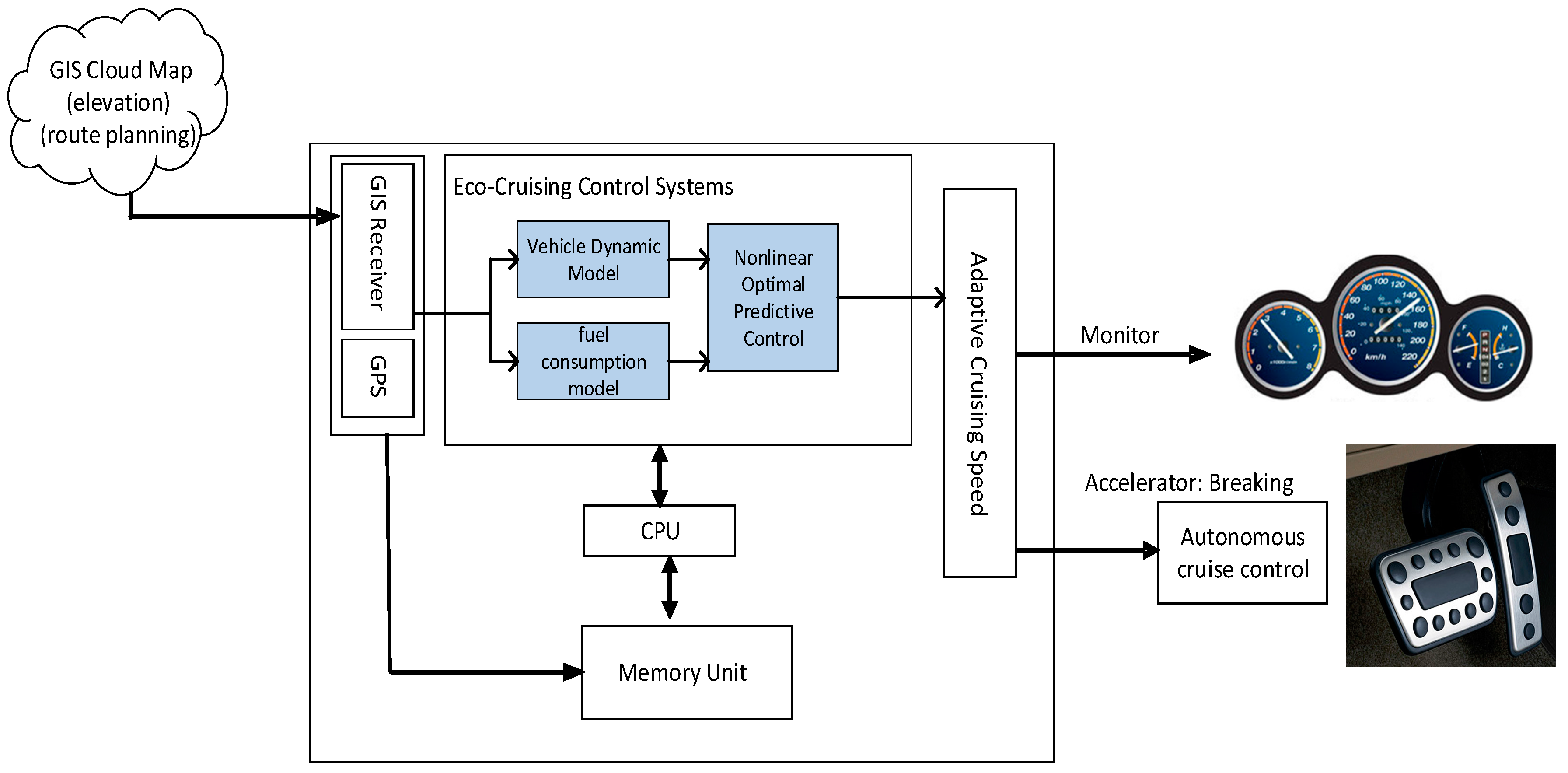
The aim of this paper is to present the eco-cruise control (ECC) system on roads with up-down slopes when there is no one in front of you the vehicle. In this paper, ride comfort and fuel economy are chosen as the main characteristics of the desired behavior of an eco-cruise control system. A nonlinear optimal predictive controller for ecological driving of using the dynamic programming with rolling horizon framework and taking a penalty function as the soft constraints with pre-specified hard limitations is proposed. It can efficiently provide superior fuel economy and ride comfort, simultaneously. The architecture of eco-cruise control system is illustrated in Figure 2.

First, the route planning and road gradient angle (elevation data) on the planned route are derived simultaneously from the Google Maps API. Here, this application uses the Google Directions API [16,17] to help us the route planning. Therefore, GPS coordinates (longitude and latitude) and elevation data for all locations on the planned route are obtained as the practical up-down road surface of vehicle dynamic model. Once the ACC forward-looking radar system detects that the forward vehicle is no longer in the host vehicle’s path, the eco-cruise control system will start automatically. In practice, the latitude and longitude coordinates of cruise vehicle current location can be obtained by GPS receiver. Thus, the position of the cruise vehicle and road altitude data of the road ahead can be known, and then they can be used to calculate the most fuel-efficient speed profile on the planned route. Knowing the above information, the proposed ECC strategy for the vehicle can increase some extra speed before entering a hill. Similarly, the proposed ECC strategy can ease off the throttle shortly to allow gravity to help the vehicle slow down before the start of a descent. Thus, the proposed ECC strategy can save most fuel.

In this paper, we proposes an efficient way of using rolling horizon dynamic programming [19,20,21] and taking a penalty functions the soft constraints as well as pre-specified hard limitations for the design of nonlinear optimal predictive controller (NOPC). A quadratic cost function is developed that considers the cruising fuel consumption model, counteracting effect of gravitational force due to the road slope, transfer effect between driving force and mechanical coupling and a penalty function as the velocity compensation. Thus, the proposed ECC system not only ensures that acceleration and braking magnitudes are kept as minimum as possible for varying road environment, but also have a high level of ride quality. Finally, the estimated eco-cruise speed can be displayed through car dashboard, as it plays an important role in driver assistance system; in addition, we will be able to achieve true autonomous driving. Thus, the eco-cruise control system can exhibit the vehicle manipulations under the given topographical information and dynamic characteristics of the test vehicle.

The rest of this section derives a method of finding elevation for the planned route, vehicle dynamic model, fuel consumption model, and therefore develops an appropriate object function based on the input and states of the systems.

2.1. Elevation Data Acquirement

In order to develop an eco-cruise control system, this approach uses the topographical data, such as road slope, by the GPS systems and digital map to control the vehicle velocity to optimize its fuel consumption. The Google Maps Elevation API [22,23] is utilized to provide elevation data for all locations on the planned route. In addition, the GPS systems can be used to obtain the current position of the vehicle and road in the case of real implementation. 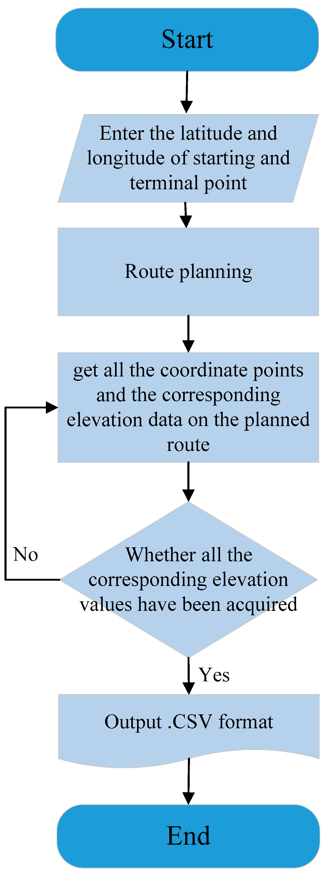Figure 3 shows the flowchart of route planning and elevation data obtainment.

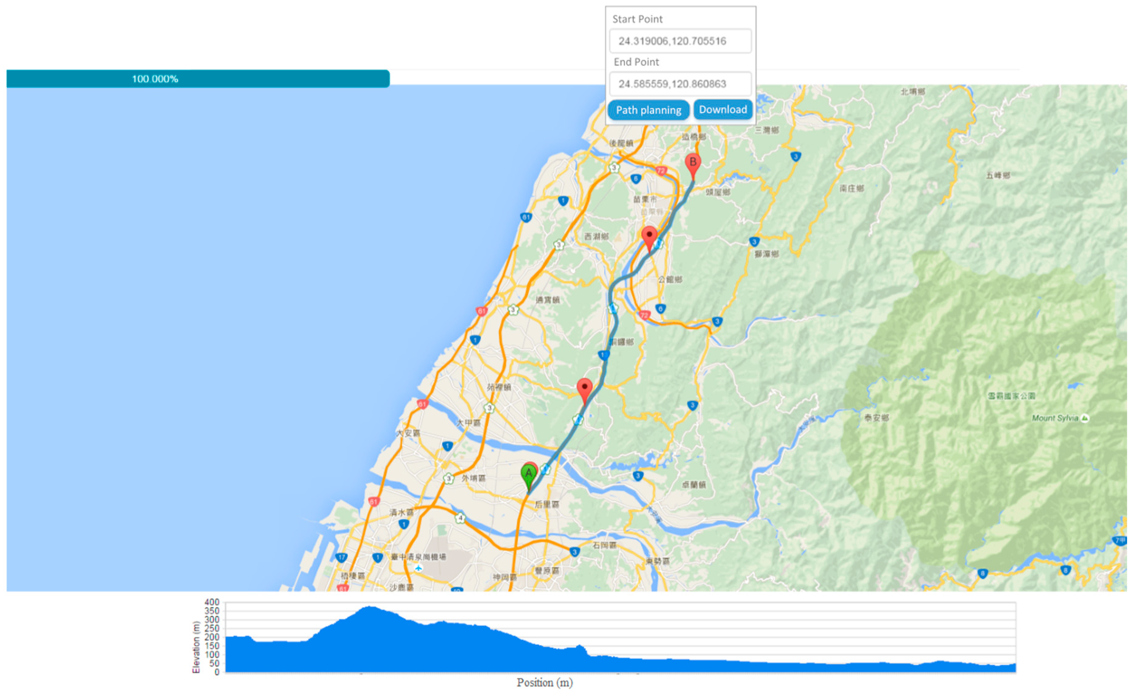
For this flowchart, we first need to enter the name of an origin and a destination or the latitude and longitude of origin and destination in our designed user interface, please see Figure 4. Then, we utilize the “Google Maps Directions API” to plan routes and to get these geographical coordinates (latitude and longitude), simultaneously. Next, according to their latitude and longitude coordinates, we apply the “Google Maps Elevation API” to obtain the elevation data for a set of locations on the planned routes. Elevation values are expressed relative to local mean sea level, which also means that altitude profile of the road in this paper. Finally, we have the whole longitude and latitude coordinates and corresponding elevation data of each location for our planned route.

Moreover, the human–machine interaction (HMI) interface based on Google Maps is designed easily to get the topographical data and to achieve the route planning. We have also built apps for both Android and iOS devices, tablets. The user interface is shown in Figure 4.

2.2. Vehicle Dynamic Modelling

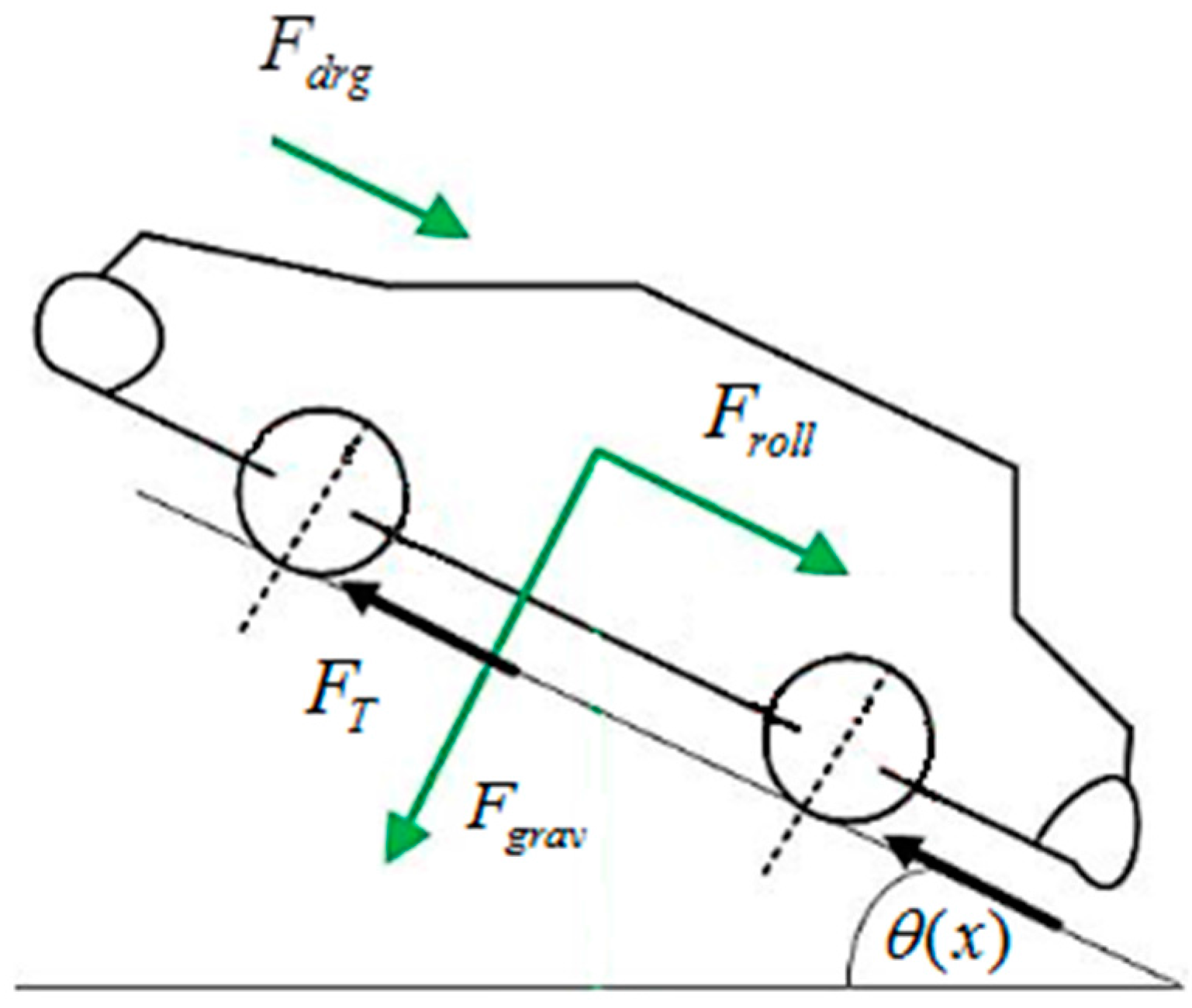
In this paper, the vehicle dynamics are expressed by the longitudinal motion of the vehicle [14] using Newton’s second law. The longitudinal forces acting on the vehicle are represented as acceleration, rolling resistance, aerodynamic drag and gravitational. These forces are shown in Figure 5. The velocity of the vehicle at any instant $t$ is subjected to the total forces acting on it, which can be modeled as below:

$$M\dot{v}(t)=F_T(t)-F_{roll}(t)-F_{drg}(t)-F_{grav}(t)$$

(1)

where $M,F_T,F_{roll},F_{drg},F_{grav}$ are the equivalent mass of vehicle including its rotating parts, the traction force, the difference between the forward friction forces and the backward rolling resistances on the tyres, aerodynamic drag, and the gravitational resistances, respectively. The three resistances are described as:

$$F_{roll}(t)=\mu Mg\cos (\theta (x)),F_{grav}(t)=Mg\sin (\theta (x)),F_{drg}(t)=\frac{1}{2}{C}_D{\rho }_a{A}_V{v}^2(t)$$

(2)

where $\mu ,C_D,{\rho }_a,A_V,\theta (x)$ are the rolling resistance coefficient, drag coefficient, air density, frontal area of the vehicle, and road slip angle as a function of position $x$ from digital map.

The traction force $F_T$ is the propulsive force that drive tire apply to the road surface to move the vehicle along a path. Here, the traction force in the vehicle is supplied by internal combustion engine (ICE) or electrical traction motor (EM). In order to express the transfer relationship between the actuator and the drive force sources, a first order system with the constant time $T$ of and delay are considered as follows:

$$F_T(t)=\frac{Cu(t)}{Ts+1}$$

(3)

where $u$ is control signal, $C=1200$ and $T=1$s. Hence, a continuous-time nonlinear system for vehicle dynamic model is defined as:

$$\{\begin{array}{l}\dot{x}(t)=v(t)\\ \dot{v}(t)=-\frac{1}{2M}{C}_D{\rho }_a{A}_V{v}^2(t)-\mu g\cos (\theta (x))-g\sin (\theta (x))+\raisebox{1ex}{$F_T(t)$}\!\left/ \!\raisebox{-1ex}{$M$}\right.\\ {\dot{F}}_T(t)=\frac{C}{T}u(t)-\frac{1}{T}{F}_T(t)\end{array}$$

(4)

Here, $u$ assuming that during the braking process, $u<0$ so no fuel is consumed.

In order to be able to implement a following predictive control procedure, the corresponding state-space description of continuous vehicle dynamic model (4) is common to convert a model to discrete time based on a sampling time $T$. Then a nonlinear discrete time difference equation of the form can be updated at a fixed interval $k$ by a digital computer.

$$\mathit{x}\left((k+1)T\right)=\mathit{x}(kT)+f\left(\mathit{x}(kT),u(kT)\right)$$

(5)

For simplicity, $T$ is omitted in the rest of this paper. In addition, ${\mathit{x}}_k={\left[\begin{array}{ccc}x& v& F\end{array}\right]}^T{|}_k$ at time step $k$ denotes the location and speed of the vehicle, and traction force, respectively. $k=0,\mathrm{...},N$ indicates the respective values at the $k\mathrm{th}$ instance in the discretized prediction horizon.

Furthermore, the road gradient angle $\theta (x)$ at location $x$ can be calculated by road elevation profile $R_{ele}$ from the Google Maps as follows:

$$\theta (x)={\tan }^{-1}\left(\frac{R_{ele}(x+\Delta x)-R_{ele}(x-\Delta x)}{2\Delta x}\right).$$

(6)

2.3. Fuel Consumption Modelling

In this paper, fuel consumption is a fairly accurate measure of a vehicle’s performance. Key factors strongly affecting fuel consumption of a vehicle are the torque and the rotational speed of the engine. To formulate the fuel consumption model, we consider a typical vehicle. It includes an engine size of about 1.3 L and a fuel consumption rate of about 17.2 km/L as per 10–15 mode fuel tests from the model catalog of the vehicle. The fuel consumption [10] in the vehicle at any velocity and acceleration can be defined as:

The fuel consumption value of a cruising vehicle is approximated by the curve-fitting process as the following polynomial [10] of the vehicle velocity:

$$f_V=b_0+b_{1}v+b_2{v}^2+b_3{v}^3+\widehat{a}\left(c_0+c_{1}v+c_2{v}^2\right)$$

(7)

where $\widehat{a}=a_v+a_{\theta }$ is the total of the obvious acceleration of the vehicle $a_v$ and the acceleration internally required to balance the decelerating force due to the road gradient ($a_{\theta }=g\sin \theta (x)$). according to (4), the obvious acceleration of the vehicle can be easily described as

$$a_v=-(\raisebox{1ex}{$1$}\!\left/ \!\raisebox{-1ex}{$2M$}\right.)C_D{\rho }_a{A}_V{\nu }^2-\mu g\cos (\theta (x))-g\sin (\theta (x))+\raisebox{1ex}{$F_T(t)$}\!\left/ \!\raisebox{-1ex}{$M$}\right.$$

(8)

At the idling condition, the vehicle velocity $\nu =0$ that means the vehicle is not controlled, but there exists a constant consumption $f_V=b_0$. By using the curve-fitting process that represents fuel consumption values at various velocities and accelerations and corresponding approximation curves, all coefficients in (7) are determined as [10]: $b_0=0.1569$, $b_1=2.450\times {10}^{-2}$, $b_2=-7.415\times {10}^{-4}$, $b_3=5.975\times {10}^{-5}$, $c_0=7.224\times {10}^{-1}$, $c_1=9.681\times {10}^{-2}$, and $c_2=1.075\times {10}^{-3}$. Thereby the fuel consumption of the vehicle can be approximated according to (7).

2.4. Nonlinear Optimal Predictive Controller Design

Nonlinear optimal predictive control (NOPC) is based on the dynamic programming principle and rolling horizon strategy to obtain the optimal feedback control gain as evaluated by a cost function for a class of constrained discrete-time systems. The result of the optimization process is the optimal predictive control sequence $\mathit{U}(k+j|k)={\left\{u(k+j|k)\right\}}_{j=0}^{N-1}$ for the control horizon $N$ at discrete time step $k$. Based on the rolling horizon strategy, only of the control sequence is applied to the (5). The rest of the control sequence is employed for plant behavior estimation by using the dynamic programming optimization. Thus, this dynamic program is repeated each time-step in a rolling horizon framework.

To consider the issue of ride comfort in eco-cruise control system, the vehicle acceleration and deceleration are directly concerned with the input force and variation of engine torque. Therefore, the control input is limited to both min-max constraints, and the formulation is:

$$u_{\min }\le u\left(k+j|k\right)\le u_{\max }$$

(9)

where $u_{\max }$ and $u_{\min }$ are the upper acceleration limit and lower acceleration limit for the vehicle, they will be assumed equal to 0.25 and −0.5 g [24], respectively. Once the control input is always varies in a bounded range, that means that the vehicle has maintained an acceptable ride quality.

Applying NOPC on (4) and considering the input constraint (9), a constrained optimal control problem is solved over a prediction horizon $N$ during each sampling period, which is using the current state $\mathit{x}(k|k)\equiv \mathit{x}(k)$ at discrete time step $k$ as the initial state. To find a sequence of control inputs, the following performance index must be minimized within a future horizon which minimizes the generalized quadratic cost function repeatedly over $k+j|k$:

$$\begin{array}{l}\underset{{\left\{u(k+j|k)\right\}}_{j=0}^{N-1}}{\min }J\left(\mathit{x}(k|k),u(k|k)\right)\\ ={\displaystyle \sum _{j=0}^{N-1}\{{\omega }_1\left[\frac{b_0+b_{1}v(k+j|k)+b_2(v^2(k+j|k))+b_3(v^3(k+j|k))}{v\left(k+j|k\right)}\right]}\\ +{\omega }_2\left[\frac{1}{2}{\left(a_v+g\sin (\theta (x(k+j|k)))\right)}^2\right]\\ +{\omega }_3\left[\frac{1}{2}{\left(v\left(k+j|k\right)-\frac{1}{2}\left(v_d+\mathrm{\Phi }\left(v^{ref}(k+j|k)\right)\right)\right)}^2\right]\\ +{\omega }_4\left[\frac{1}{2}{\left(u(k+j|k)-\frac{F_T(k+j|k)}{M}\right)}^2\right]\}\\ \mathrm{Subject}\mathrm{to}:\mathrm{Equation}\left(5\right)\end{array}$$

(10)

where ${\omega }_1,{\omega }_2,{\omega }_3,{\omega }_4$ denote the constant weights; $\mathrm{\Phi }\left(v^{ref}(k+j|k)\right)$ denotes the penalty function; $N$ denotes the output and control horizon; $v_d$ denotes the a steady cruising speed as set by the driver; $v^{ref}$ denotes the cruising speed form the nominal cruise control system on hilly roads (without considering the penalty function). In (10), the cost function includes of three parts. First expresses the cost in relation to the cruising fuel consumption, which is derived from (7) and setting $\widehat{a}=0$. The cost function of second part means that corresponds to the acceleration effect of the vehicle, which including acceleration force and gravitational counteracting force due to the road slope. Third part is the cost for cruising speed compensation with regard to the road slope, where $\mathrm{\Phi }(v^{ref}(k+j|k))$ is a penalty function, it can be represented as

$$\mathrm{\Phi }(v^{ref}(k+j|k))=\{\begin{array}{cc}\max \left(v_d+(v_d-v^{ref}(k+j|k))\right),& \theta (x(k+j|k))>0,\\ 0,& \theta (x(k+j|k))=0,\\ \min \left(v_d+(v_d-v^{ref}(k+j|k))\right),& \theta (x(k+j|k))<0\end{array}$$

(11)

The penalty function $\mathrm{\Phi }(v^{ref}(k+j|k))$, enforcing as the soft constraints, is penalized along with the cruising speed limit when driving the uphill or downhill. The last part is the cost of that corresponds to the transfer effect between the actuator and the driving force. Note that the proper weight selection, it can be slightly tuned by direct observation of the simulation results to minimize the fuel consumption when driving on roads with up-down slopes.

From (10), it is essential to derive an optimal control law with the initial state $\mathit{x}(k|k)$. In order to solve the optimal control input at discrete time step $k$, the Hamiltonian function is formulated using (5) and (10) for the $j=0,\mathrm{...}N-1$ as follows:

$$\begin{array}{l}H\left(\mathit{x}(k+j|k),\mathbf{\lambda }(k+j|k),u(k+j|k)\right)=L\left(\mathit{x}(k+j|k),u(k+j|k)\right)\\ +{\mathbf{\lambda }}^T\left(k+j+1|k\right)\left(\mathit{x}(k+j|k)+f\left(\mathit{x}(k+j|k),u(k+j|k)\right)\right)\end{array}$$

(12)

where $\mathbf{\lambda }(k)={\left[\begin{array}{ccc}{\lambda }_1& {\lambda }_2& {\lambda }_3\end{array}\right]}^T{|}_k\in {\Re }^n$ is a Lagrange multiplier vector sequence. Therefore, stationarity condition and co-state equations for state $\mathit{x}(k)=\left[\begin{array}{ccc}x& v& F\end{array}\right]{|}_k$ are thus respective given by

$$\begin{array}{l}\frac{\partial H}{\partial u(k+j|k)}=0,{\lambda }_1(k+j|k)=\frac{\partial H}{\partial x(k+j|k)},\\ {\lambda }_2(k+j|k)=\frac{\partial H}{\partial v(k+j|k)},{\lambda }_3(k+j|k)=\frac{\partial H}{F_T(k+j|k)}\end{array}$$

(13)

According to stationarity condition, the solution of the rolling horizon optimal control problem exists and the feedback control is given by

$$u^{\ast }(k+j|k)=-\frac{{\lambda }_3(k+j+1|k)C}{{\omega }_{4}T}+\frac{F_T(k+j|k)}{M}$$

(14)

The control law is implemented in a rolling horizon manner, meaning that at every step $k$, an optimal future control input sequence ${{\mathit{U}}^{\ast }}_{k+j|k}={\left\{u^{\ast }(k+j|k)\right\}}_{j=0}^{N-1}$ by applying dynamic programming strategy can be derived in the sense of the minimization cost function (10). Note that since the road slope angle $\theta (x)$ is the function of only $x$, to solve this optimal control input, we need to computer the co-state equations previously. According to (13), the terminal term of $\mathbf{\lambda }\left(k+j|k\right)$ can reasonable to assume $\mathbf{\lambda }\left(k+N|k\right)=0$ when $j=N-1$ for discrete time step $k$. By using the iteration method, the co-state sequence $\mathbf{\lambda }\left(k+j|k\right)$ and control input sequence ${\mathit{U}}^{\ast }(k+j|k)$ for $j=0,\mathrm{...}N-1$ can be obtained by the optimization process. Therefore, a state feedback control sequence by using (14) at discrete time step $k$ can be written as

$${\mathit{U}}^{\ast }(k+j|k)=\left[\begin{array}{c}{u}^{\ast }(k+0|k)\\ u^{\ast }(k+1|k)\\ ⋮\\ u^{\ast }(k+N-1|k)\end{array}\right],j=0,\mathrm{...},N-1$$

(15)

According to the receding horizon implementation, only the first element of the optimal predicted input sequence ${\mathit{U}}^{\ast }(k+j|k)$ is input to the systems plant (5), as

$$u_k=u^{\ast }(k|k)$$

(16)

where $u^{\ast }(k|k)=u^{\ast }(k+0|k)$. Note that since the optimal control law $u^{\ast }(k+j|k)$ is constrained to lie in an admissible region; therefore, the hard constraints (9) have to be satisfied. if $u^{\ast }(k+j|k)$ is larger than $u_{\max }$, we should select $u^{\ast }(k+j|k)=u_{\max }$ as a largest possible optimal control input. On the other hand, if $u^{\ast }(k+j|k)$ is less than $u_{\min }$, we should select $u^{\ast }(k+j|k)$ as its minimum admissible value of $u_{\min }$. If $u^{\ast }(k+j|k)$ is bounded on $\left[u_{\min },u_{\max }\right]$, then $u^{\ast }(k+j|k)$ is an optimum control input at discrete time step $k$. Hence,

$$\tilde{u}(k+j|k)=\{\begin{array}{cc}{u}_{\max },& u^{\ast }(k+j|k)\ge u_{\max }\\ u^{\ast }(k+j|k),& u_{\min }<u^{\ast }(k+j|k)<u_{\max }\\ u_{\min },& u^{\ast }(k+j|k)\le u_{\min }\end{array}$$

(17)

That is the minimum energy constrained-input control expressed as a co-state feedback. Thus, the vehicle can enhance ride comfort, even have better fuel economy.

2.5. Stability Analysis

For stability analysis, it should be noted that the NOPC controller is locally stabilizing the discrete-time systems in (5). We shall utilize the Lyapunov function theory to analyze the asymptotic stability criteria for our proposed the Eco-cruise control system.

Theorem 1.

Consider the discrete-time closed-loop systems (5) with the Lyapunov functional.

$$V\left(\mathit{x}(k|k)\right)\equiv \underset{{\left\{u(k+j|k)\right\}}_{j=0}^{N-1}}{\min }J\left(\mathit{x}(k|k),u(k|k)\right)$$

(18)

Suppose there exist ${\omega }_i\ge 0$ for $i=1,\mathrm{...},4$ for each discrete time step such that satisfying the following

$$\begin{array}{l}{\displaystyle \sum _{j=0}^{N-1}\{{\omega }_1\left[\frac{b_0+b_{1}v(k+j|k)+b_2(v^2(k+j|k))+b_3{v}^3((k+j|k))}{v\left(k+j|k\right)}\right]}\hfill \\ +{\omega }_2\left[\frac{1}{2}{\left(a_v+g\sin (\theta (x(k+j|k)))\right)}^2\right]+{\omega }_3\left[\frac{1}{2}{\left(v\left(k+j|k\right)-\frac{1}{2}\left(v_d+\mathrm{\Phi }\left(v^{ref}(k+j|k)\right)\right)\right)}^2\right]\hfill \\ +{\omega }_4\left[\frac{1}{2}{\left(u(k+j|k)-\frac{F_T(k+j|k)}{M}\right)}^2\right]+\nabla V_{k+j|k}^T\left(\mathit{x}(k+j+1|k)-\mathit{x}(k+j|k)\right)\}=0\hfill \end{array}$$

(19)

where $\nabla V_{k+j|k}^T(\mathit{x})$ is the gradient vector for each $\mathit{x}\left(k|k\right)$, then systems (5) subjected to the optimal control law described by (14) would be asymptotically stable.

Proof. 

Assume that $V\left(\mathit{x}(k|k)\right)>0$ exist and is continuously differentiable. Then

$$V\left(\mathit{x}(k+N|k)\right)-V\left(\mathit{x}(k|k)\right)={\displaystyle \sum _{j=0}^{N-1}\Delta V\left((k+j|k)\right)}$$

(20)

As we know, $\Delta V(\mathit{x}(k+j|k))=V\left(\mathit{x}(k+j+1|k)\right)-V\left(\mathit{x}(k+j|k)\right)$ can be expressed as the first difference. Since $V\left(\mathit{x}(k|k)\right)$ is assumed a continuously differentiable function; therefore, $V\left(\mathit{x}(k|k)\right)$ can be expanded by using Taylor series about the operating point of $\mathit{x}\left(k|k\right)$ renders

$$V\left(\mathit{x}(k+j+1|k)\right)=V\left(\mathit{x}(k+j|k)\right)+\nabla V_{k+j|k}^T\left(\mathit{x}(k+j+1|k)-\mathit{x}(k+j|k)\right)$$

(21)

where

$$\begin{array}{ll}\nabla V_{k+j|k}(\mathit{x})& ={\raisebox{1ex}{$\partial V\left(\mathit{x}\right)$}\!\left/ \!\raisebox{-1ex}{$\mathit{x}$}\right.|}_{\mathit{x}=\mathit{x}(k+j|k)}\\ & ={{\left[\begin{array}{ccc}\raisebox{1ex}{$\partial $}\!\left/ \!\raisebox{-1ex}{$\partial x(k)$}\right.V(\mathit{x})& \raisebox{1ex}{$\partial $}\!\left/ \!\raisebox{-1ex}{$\partial v(k)$}\right.V(\mathit{x})& \raisebox{1ex}{$\partial $}\!\left/ \!\raisebox{-1ex}{$\partial F_T(k)$}\right.V(\mathit{x})\end{array}\right]}^T|}_{\mathit{x}=\mathit{x}(k+j|k)}\end{array}$$

(22)

Therefore, we can know that

$$\Delta V\left(\mathit{x}(k+j|k)\right)\approx \nabla V_{k+j|k}^T\left(\mathit{x}(k+j+1|k)-\mathit{x}(k+j|k)\right)$$

(23)

Observing (23) and (20), the (23) can rewritten as

$$V\left(\mathit{x}(k+N|k)\right)-V\left(\mathit{x}(k|k)\right)={\displaystyle \sum _{j=0}^{N-1}\nabla V_{k+j|k}^T\left(\mathit{x}(k+j+1|k)-\mathit{x}(k+j|k)\right)}$$

(24)

Adding (24) on both sides of (10) such that

$$\begin{array}{l}J\left(\mathit{x}(k|k),u(k|k)\right)-V\left(\mathit{x}(k|k)\right)\\ ={\displaystyle \sum _{j=0}^{N-1}\{{\omega }_1\left[\frac{b_0+b_{1}v(k+j|k)+b_2(v^2(k+j|k))+b_3{v}^3((k+j|k))}{v\left(k+j|k\right)}\right]}\\ +{\omega }_2\left[\frac{1}{2}{\left(a_v+g\sin (\theta (x(k+j|k)))\right)}^2\right]\\ +{\omega }_3\left[\frac{1}{2}{\left(v\left(k+j|k\right)-\frac{1}{2}\left(v_d+\mathrm{\Phi }\left(v^{ref}(k+j|k)\right)\right)\right)}^2\right]\\ +{\omega }_4\left[\frac{1}{2}{\left(u(k+j|k)-\frac{F_T(k+j|k)}{M}\right)}^2\right]+\nabla V_{k+j|k}^T\left(\mathit{x}(k+j+1|k)-\mathit{x}(k+j|k)\right)\}\\ -V\left(\mathit{x}(k+N|k)\right)\end{array}$$

(25)

Thus, according to (18) and (24), one may conclude the existence of the above (19), it can easily obtain that

$$\begin{array}{l}\Delta V\left(\mathit{x}(k+j|k)\right)=V\left(\mathit{x}(k+j+1|k)\right)-V\left(\mathit{x}(k+j|k)\right)\\ =-{\omega }_1\left[\frac{b_0+b_{1}v(k+j|k)+b_2{(v(k+j|k))}^2+b_{3}v{((k+j|k))}^3}{v(k+j|k)}\right]\\ -{\omega }_2\left[\frac{1}{2}{\left(a_v+g\sin (\theta (x(k+j|k)))\right)}^2\right]\\ -{\omega }_3\left[\frac{1}{2}{\left(v\left(k+j|k\right)-\frac{1}{2}\left(v_d+\mathrm{\Phi }\left(v^{ref}(k+j|k)\right)\right)\right)}^2\right]\\ -{\omega }_4\left[\frac{1}{2}{\left(u(k+j|k)-\frac{F_T(k+j|k)}{M}\right)}^2\right]\\ \le 0\end{array}$$

(26)

It is clear to prove that (19) satisfies the assumption of Theorem 1. This implies that the difference of $V\left(\mathit{x}(k|k)\right)$ along the systems trajectory is negative. Thus, the systems (5) controlled by (14) is asymptotically stability. This proof is ultimately complete.

3. Results and Discussion

The objective of this section is to evaluate the performance of the proposed NOPC approach for eco-cruise control system. The three traffic scenarios are carried out with a discrete-time longitudinal vehicle model, whose simulation results are shown below. The vehicle dynamic model is defined by (4), which has the following parameters: $M$ is 1200 kg; ${\rho }_a$ is 1.184 $\mathrm{kg}/{\mathrm{m}}^3$; $A_V$ is 2.5 $m^2$; $C_D$ is 0.32, and $\mu$ is 0.015. To further evaluate the energy-saving performance of the proposed eco-cruise control system, the fuel consumption model is also considered. For comparison of performance, a traditional cruise control system, meaning the fixed speed driver strategy (FSD), is also designed based on the same control plant. In this paper, a notation eco-cruise control (ECC) strategy is used to indicate a vehicle, which is designed by the proposed NOPC algorithm for eco-driving.

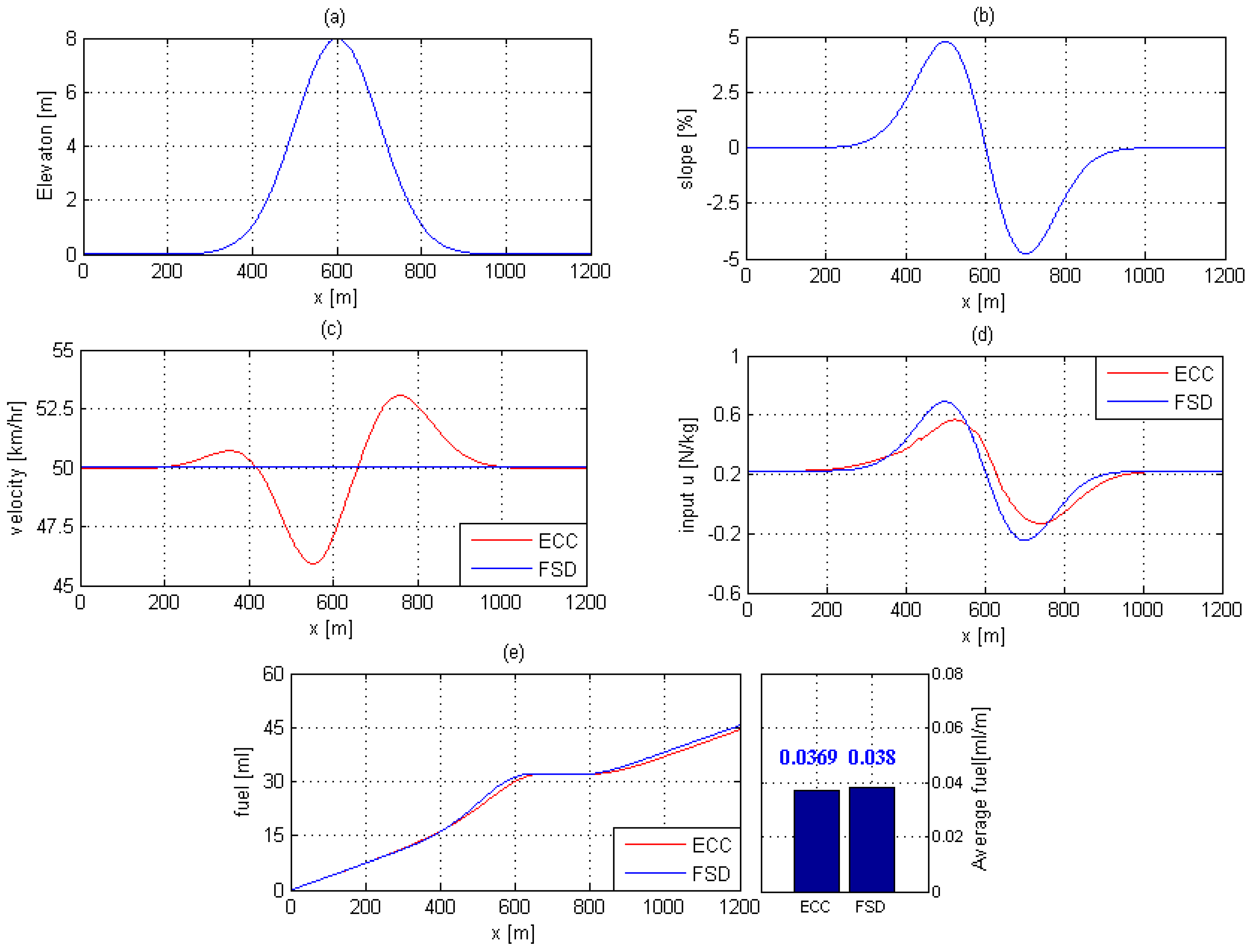
3.1. Case 1. Road with Up-down Slope Scenario

The first scenario considers that the typical driving scenarios on the road with up-down slope. The total length of road is 1200 m, the maximum altitude is 8 m and the cruising speed is initially set at a velocity of 50 km/h.

As seen in Figure 6c, the vehicle of ECC strategy slightly increases the cruising speed before entering a hill. Similarly, the vehicle of ECC strategy can ease off the throttle shortly to allow gravity to help the vehicle slow down, with the help of momentum and weight, and without any braking. In addition, Figure 6d shows that the ECC strategy superior ride comfort than FSD strategy. Figure 6e illustrates that the total fuel consumption of ECC strategy and FSD strategy are 44.24 mL and 45.55 mL; the FSD strategy required precisely 2.96% of extra fuel, compared with the ECC strategy, respectively. Moreover, the average fuel consumption of ECC strategy can reduce 2.98% than FSD strategy.

3.2. Case 2. Road with Down-up Slope Scenario

In this case, the vehicle travels on the roads with down-up slopes. The cruising speed of the vehicle is initially set at a velocity of 50 km/h, and the total length of road and maximum altitude are 1200 m and −8 m, respectively. The simulation and comparison results for this scenario are presented in Figure 7.

As observed in Figure 7e, the total fuel consumption and average fuel consumption in case 2 have better than case 1 because there is no necessity of braking when the vehicle starts in a descent, which means that it can substantially reduce fuel wastage. It is found that the total fuel consumption of ECC strategy and FSD strategy are 43.46 mL and 45.54 mL; precisely, the FSD strategy required 4.78% of extra fuel, compared with the ECC strategy, respectively. Overall, the average fuel consumption is reduced by 4.1% for the drives with NOPC recommendation, compared to the FSD strategy. Therefore, it can be concluded that the ECC strategy is able to maintain an ecological speed and ride comfort while improving the performance of the vehicle.

3.3. Case 3. Virtually Real Road Scenario

Finally, a virtually real road is utilized to evaluate the effectiveness of the proposed eco-cruise control system. The testing route is a Taiwan’s highway, which is located in Sanyi Township, Miaoli County, Taiwan, R.O.C., and the length about 25 km, which testing route can be described as Figure 4. Moreover, the road elevation profile is derived by Google Maps, and the road profile is illustrated in Figure 8a. There are up-down hilly areas with different shapes in the proposed real route.

In the case of driving in the real road scenario, the results show that the total fuel consumption of ECC strategy and FSD strategy are 1631 and 1682 mL, respectively. The proposed eco-cruise control system has saved 3.13% fuel consumption in comparison with the conventional cruise control system. In addition, the average fuel consumption has also reduced by 4.1% for the drives with NOPC, compared with the FSD strategy, respectively.

The above simulation results for two different control strategies under different driving scenarios are shown in following

Table 1. Comparison of the fuel economy for two control strategies.

Item	Case 1		Case 2		Case 3
	FSD	ECC	FSD	ECC	FSD	ECC
Total road length	1.2 km		1.2 km		25 km
Total fuel consumption	45.55 mL	44.24 mL	45.54 mL	43.46 mL	1682 mL	1631 mL
Average fuel consumption	26.34 km/L	27.12 km/L	26.35 km/L	27.61 km/L	14.86 km/L	15.32 km/L
Economy rate		2.96%		4.78%		3.13%

. The results show that the ECC system can provide better fuel economy than traditional cruise control system, up to 2%–4% better fuel economy. These results in fuel saving reveals the creditability of such ecological driving based on ECC design strategy.

4. Conclusions

This paper proposes a nonlinear optimal predictive control (NOPC) law for design of an eco-cruise control system based on GPS and digital topographical data. Considering the longitude vehicle dynamics and fuel consumption model, theoretical development and numerical verification show that the proposed discrete-time NOPC strategy is feasible for implemented to generate appropriate control inputs to get the comfortable driving, better fuel economy and increase the cruising stability, simultaneously. For the proposed eco-cruise control system, the updating NOPC law trends to an improved control force which renders a suboptimal control. Based on the Lyapunov stability theory, a guaranteed cost control law is also developed to ensure systems stability when state and control constraints are simultaneously considered.

Simulation results illustrate that for the vehicle driving over a hill, the proposed ECC strategy takes advantage of the elevation data through Google Maps to increase the vehicle speed before the uphill. On the other hand, before the downhill, the vehicle can ease off the throttle shortly to allow gravity to help the vehicle slow down, with the help of momentum and weight, and ease down the hill. Therefore, the ECC strategy can save most fuel. In the future, we believe that the approach holds great promise to a wide range of realistic problems.