
Advanced Spatial Modeling to Inform Management of Data-Poor Juvenile and Adult Female Rays


1
Marine and Freshwater Research Centre, Galway-Mayo Institute of Technology, Galway, Co. Galway, Ireland
2
Marine Institute, Oranmore, Co. Galway, Ireland
*
Author to whom correspondence should be addressed.
Fishes 2017, 2(3), 12; https://doi.org/10.3390/fishes2030012
Submission received: 20 June 2017
/
Revised: 21 July 2017
/
Accepted: 21 July 2017
/
Published: 4 August 2017
Abstract
:Chronic overfishing has depleted numerous elasmobranch stocks in the North East Atlantic, but addressing this issue has been hampered by management complications and lacking data. Spatial management approaches have thus been advocated. This work presents a novel application and further development of an advanced spatial modeling technique to identify candidate nursery grounds and spawning areas for conservation, by subsetting already limited data. Boosted Regression Tree models are used to predict abundance of juvenile and mature female cuckoo (Leucoraja naevus), thornback (Raja clavata), blonde (Raja brachyura), and spotted (Raja montagui) rays in the Irish Sea using fish survey data and data describing fishing pressure, predation and environmental variables. Model-predicted spatial abundance maps of these subsets reveal distinct nuances in species distributions with greater predictive power than maps of the whole stock. These resulting maps are then integrated into a single easily understood map using a novel approach, standardizing and facilitating the spatial management of data-limited fish stocks.
Keywords:
boosted regression trees; BRT; elasmobranch; marine protected area; MPA; nursery area; spawning ground; ray1. Introduction
Decades of overfishing have significantly impacted the diversity of North-East Atlantic ecosystems, and markedly reduced the numbers of large ray species [1,2,3]. The large size and low fecundity of elasmobranchs such as rays makes them especially vulnerable to fishing pressure [4,5,6]. As a result of high fishing effort, the Irish Sea now supports fewer of each species of ray, which are of smaller average size, and inhabit smaller areas, than ever before [1,7,8]. The study species—cuckoo ray Leucoraja naevus, thornback ray Raja clavata, blonde ray Raja brachyura and spotted ray Raja montagui—are classed as either “data-limited” (blonde ray) or have enough surveyed data to reveal trends (the other species) [9], based on data collected annually in the ICES (International Council for the Exploration of the Sea) IBTS (International Bottom Trawl Survey) [10]. Conservation efforts for these species are complicated by inconsistencies in how the stocks are managed, both spatially and temporally [11].
They are managed under a joint Total Allowable Catch (TAC) limit (with small-eyed (Raja microocellata), sandy (Leucoraja circularis) and shagreen ray (Leucoraja fullonica)) for the geographical stock areas of waters west, northwest and southwest of the UK and Ireland [12], and in the Irish Sea are mainly taken as bycatch to the TR1 métier (otter trawl and demersal seine with mesh size ≥100 mm) fleet, and also targeted by a dwindling Irish fleet of three vessels or fewer. The spatial distribution of fishing effort is relatively annually stable, principally centered around the offshore banks east of Dublin. Scientific advisors have called for appropriate [13], and Maximum Sustainable Yield-based (MSY) management of all stocks by 2020 [14], and have recommended that novel spatial management approaches be explored [15]. This would ideally be done with length-based indicators [16]. Specifically, protection of spawning and/or nursery grounds has been proposed as a potential spatial management solution to conserve these species [15,17,18,19].
Spatial management requires an understanding of the spatial distribution of these species. Various spatial analysis approaches exist, such as Generalised Linear/Additive Modelling (GLM/GAM) [20,21] also [22], and references therein, MARXAN [23,24,25], and MaxEnt [26,27]. Among these, Boosted Regression Trees (BRTs) show the greatest ability to model data-limited fish stocks (see [11,16,28] for comparisons). This technique combines boosting (averaging multiple rough predictors) with introduced stochastic training (bagging), with regression trees progressively focusing on remaining poorly modeled observations. Automated BRT modeling approaches have demonstrated an ability to provide robust spatial abundance predictions for these and similar species, and have been used to identify environmental correlates of distribution and abundance, using whole-stock datasets [11]. However, the rudimentary approach to synthesizing multiple outputs in that study could be improved with an automated approach that mathematically joins the various subset outputs, scales to the least abundant subset and weighted based on user preference. This will allow marine managers to assess conservation options by using a single precise map for multiple species and/or life history stages, adding another layer of understanding while retaining the multiple individual species/subset maps generated by default during the gbm.auto modeling process (see Section 4.3; full list of R functions and packages used in Appendix A).
Currently, a voluntary plan for spawning-season closed areas has been only minimally implemented and has not been evaluated [16]; preliminary work has seen nominal nursery areas and proxy spawning grounds mapped using simple point data from the observer program [29]. This study develops novel spatial predictive models of rays’ Catch Per Unit Effort (CPUE) as a proxy for their abundance in the Irish Sea. The method generates spatial CPUE prediction maps for these four species of ray across the Irish Sea based on direct fishing pressure, eggcase removal agents (scallop dredging effort and whelk Landings Per Unit Effort (LPUE)), fish predator CPUE, and environmental characteristics. We use the BRT method developed by [11] to identify priority areas for the conservation of vulnerable components/subsets of the population (mature females and juveniles), and test whether the inclusion of relative measures of fishing effort, predation and egg case removal can improve predictions of ray CPUE compared to a model based only on environmental predictors. Finally, we sum the predicted CPUE maps for juvenile and mature female rays at each site to amalgamate both sets of maps, and then amalgamate those joint maps for all four species, using a novel technique. This results in a single synthesis map of ray conservation value to inform the spatial management of data-limited rays in the Irish Sea.
If these maps accurately convey the information contained in the original predicted CPUE maps that produced them, this could obviate the need to assess each set of maps individually, saving time and effort. Such maps will be more informative to managers than synthesis maps produced using the authors’ earlier methodology [11], a key aim for this work.
2. Results
2.1. Relative Importance of Explanatory Variable Types
The summed influence score for environmental variables was twice as great as fish predator CPUE for the analysis of the juvenile subset (Figure 1, sixth and subsequent bars), and eggcase-reducing agents (whelk catch rate and scallop effort) had only a minor influence (6.5%). There was no relationship between commercial fishing pressure (LPUE) and surveyed juvenile or adult females ray occurrence and CPUE (Figure 1). See Table 3 for a list of the explanatory variables used in this study, their spatial resolutions and sources.
2.2. Influential Variable Relationships and Predicted CPUE Maps
Predicted CPUE surfaces are presented in Figure 2, and Figure S2a–i for per-species binary and Gaussian bar charts of variable influence, and line plots of individual variable/response relationships for presence/absence and CPUE.
2.2.1. Cuckoo Ray
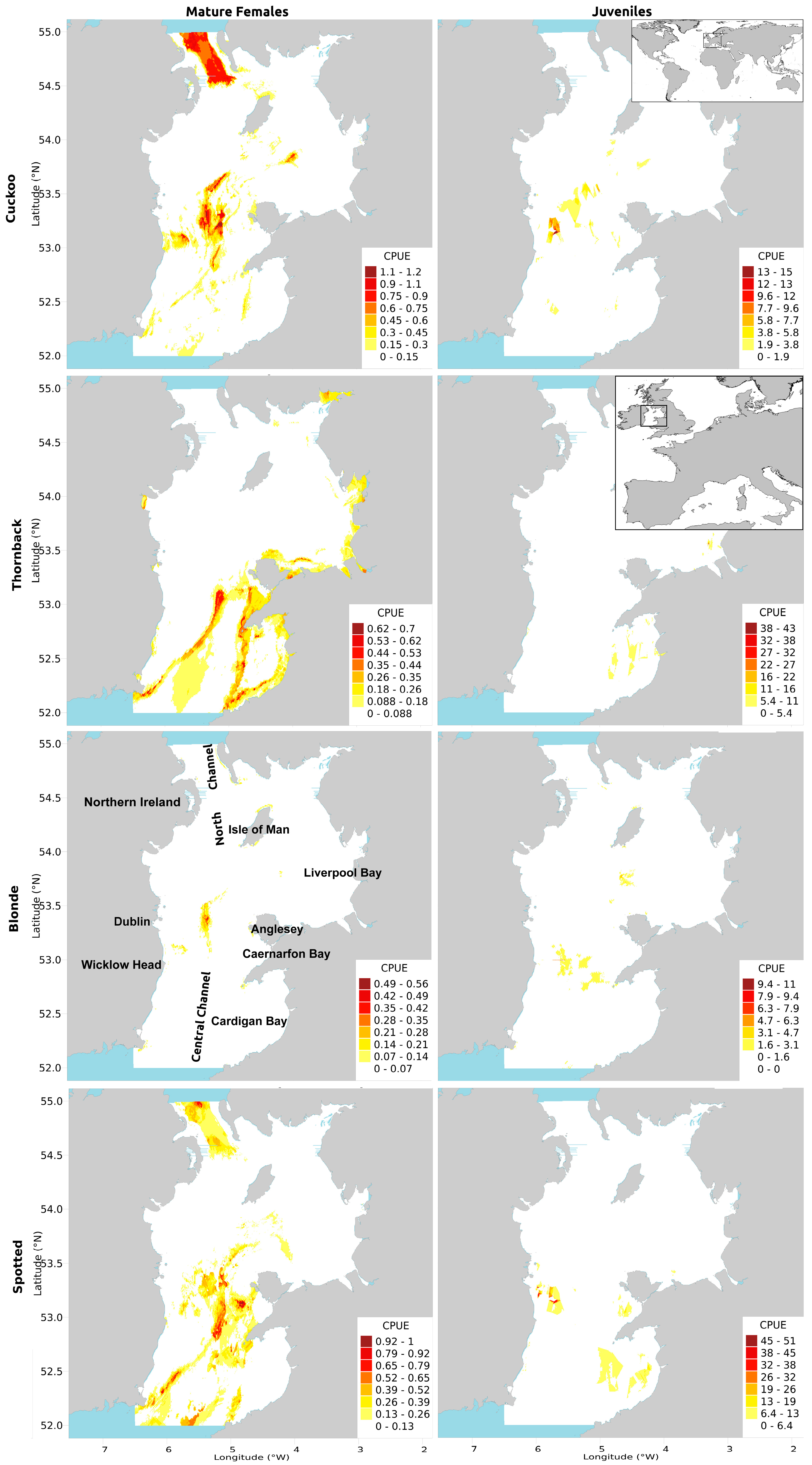
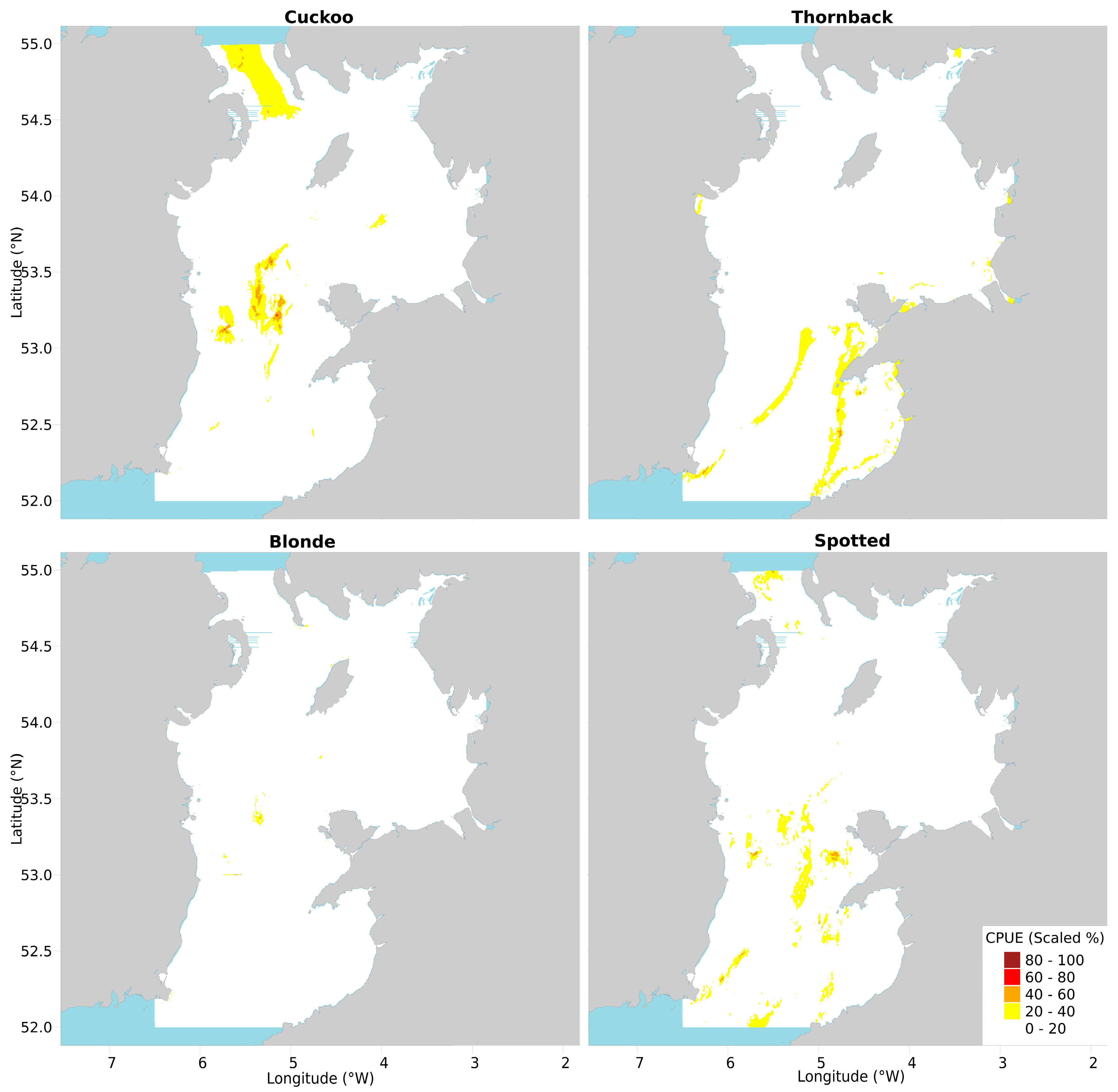
The presence/absence and CPUE of mature female cuckoo ray was best predicted by depth (>100 m), distance to shore (mostly increasing with distance offshore but greatest at 44 km), and current speed (especially >1 m s−1), similar to the results for all cuckoo rays found by [11] (see that paper’s Supplementary Materials). Highest CPUE was predicted in the middle of the deeper Central Channel, and in the North Channel.
The presence/absence of juveniles was best predicted by haddock CPUE (small ray presence peak at 12 haddock per hour, then a trough, then positive correlation, until reaching a plateau above 40 haddock per hour), current speed (presence rising sharply above 0.8 m s−1) and distance to shore (positive relationship, almost exponential in appearance, peak at 38 km then final peak and plateau above 48 km). Juvenile CPUE was best predicted by grain size (preference for sand/gravel), blonde rays (positive relationship), and haddock (positive relationship with peak ray CPUE at ~50 haddock per hour, then dropping ray CPUE with continually climbing haddock numbers; Figure S2e). While the model predicted high CPUEs in similar areas to adult females, CPUE was more strongly concentrated in smaller, more distinct central regions within the Central Channel and off the southwest coast of the Isle of Man.
2.2.2. Thornback Ray
Mature female thornback ray presence/absence and CPUE were best predicted by salinity (increasing with increasing salinity), depth (greatest at ~40 and 100–120 m) and temperature (strong preference for waters warmer than 16 °C). Highest CPUE of thornback rays was predicted in a band running from the southeastern tip of Ireland to Anglesey, and down across Cardigan Bay, as well as in the near-shore areas in both of the Eastern bays. While these findings concur with those of [11], bands of high CPUE were more pronounced.
Juvenile presence/absence and CPUE were best predicted by plaice CPUE (CPUE of thornback rays increasing with plaice CPUE, peaking at ~200 plaice per hour and then dropping to a plateau) (Table 1), temperature (preference rising sharply above 16 °C), and salinity (avoidance between 33.4–34.2 ppm, peak preference at 34.3–34.6 ppm; Figure S2g). Areas of peak predicted CPUE were in small distinct near-shore regions around Anglesey and Liverpool Bay.
2.2.3. Blonde Ray
Mature female blonde ray presence/absence and CPUE were best predicted by current speed (peak between 1 and 1.2 m s−1), depth (<30 m or >90 m) and temperature (preference for colder waters but also at 15 °C). High CPUE of blonde rays was predicted in two discrete patches within the Central Channel and just off the near-shore Irish banks.
Juvenile presence/absence and CPUE was best predicted by depth (aversion to the 40–65 m range), current speed (positive relationship), and temperature (positive relationship but with a sub-peak at the midrange 15.5 °C; Figure S2h). Predicted areas of high CPUE are very similar to those of mature females, though slightly higher in the southern Central Channel. The vertical line of high predicted abundance around 53° N coincides with the bottom of an ICES rectangle. This plotting artifact occurs because the whelk and scallop data are recorded at the resolution of an ICES rectangle.
2.2.4. Spotted Ray
Mature female spotted ray presence and CPUE was best predicted by current speed (>0.9, peaking at 1.2 m s−1), depth (peaks at 75 and >100 m) and salinity (>34 ppm). The highest CPUEs of spotted rays were patchily distributed around the Central Channel, especially at the northern and southern extremes, and off Caernarfon Bay.
Presence/absence and CPUE of juvenile spotted ray was best predicted by plaice CPUE (ray CPUE peaks at 300 and 1050 plaice per hour, with a trough between) and salinity (peak at 34.4 ppm then high afterwards; Figure S2i). This resulted in a few specific patches of high CPUE being predicted in the spatial distribution. The spatial distribution for juveniles features distinct patches of high CPUE in the South-Eastern bays and off the sandbanks by the Central Channel, compared to adult females, which have smoothly blending gradients of predicted high CPUE.
2.2.5. Fish Predators and Eggcase Removers
Aside from the most important explanatory variables listed above, fish predator and eggcase removal predictors showed varying levels of influence on the presence/absence and CPUE of juveniles of these four rays (Table 1).
Larger rays (blonde and thornback, adult total lengths 114 and 105 cm respectively) are only significantly influenced by one predator/eggcase remover each, whereas the smaller rays (cuckoo and spotted, adult total lengths 71 and 80 cm respectively) are influenced by four (Table 1). Predicted CPUE surfaces are presented in Figure 2, and Figure S2a–i for per-species binary and Gaussian bar charts of variable influence, and line plots of individual variable/response relationships for presence/absence and CPUE.
2.3. Conservation Value Maps
2.3.1. Cuckoo Ray
The combination map (see Materials and Methods for details of the construction of this figure) prominently featured high CPUE areas that were also evident in the original maps, such as in the North Channel and patches in the Central Channel. However, some areas of high-CPUE that were prominent in the original maps were less apparent in the combined map; for example, the high-CPUE areas in the Central Channel and North Channel were reduced in size. The various small peaks in juvenile CPUE were mostly downplayed unless they happened to overlap with mature female peaks (Figure 3, including for subsequent species in this section).
2.3.2. Thornback Ray
Mature female thornback rays’ CPUE peaks were mostly in offshore bands, whereas juveniles were small near-shore pockets around Cardigan Bay, Caernarfon Bay, and Anglesey: the combination map assimilates all of this information well.
2.3.3. Blonde Ray
Mature female blonde rays were solely concentrated in the middle of the Central Channel, off the various banks there; juveniles were found there but also in a low-CPUE patch offshore in the southern Central Channel. The mid-Central Channel CPUE peak dominated the combination map, with only one thin stripe of predicted high CPUE remaining in the Southern channel.
2.3.4. Spotted Ray
Mature female spotted rays were distributed in offshore bands fringing bays like thornback rays, and in a band in the North Channel and patches in the mid-Central Channel like cuckoo rays. The juveniles were distributed in discrete blocks in the Southern Irish Sea. The combination map therefore prioritized the areas where both original maps’ CPUE peaks overlapped, which led to bands and patches in the Southern Irish Sea.
Amalgamating all eight predicted CPUE maps (juvenile and adult female for four species) into one (Figure 4) revealed the extent to which their predictions overlapped. Only two core areas of universally high CPUE remained, notably the Central Channel North-South streak and the patches east of the Irish Banks, around 53.1° N. Patches of moderate CPUE were clear from the various original maps, such as the offshore and North Channel bands from thornback and cuckoo maps.
2.4. Model Performance Metrics
For mature females, the high training data Area Under the Receiver-Operator-Characteristic Curve (AUC) scores indicate excellent discrimination of probabilities between presence and absence samples, i.e., the predictive power of the presence/absence model is high. This is also true for the Cross-Validated (CV) AUC scores, with relatively minor decrease from training to CV AUC scores, indicating that overfitting was not a serious issue and predictions were more likely to be correct [30]. These scores indicate that we can have confidence in the model predictions. See Table 2 for model performance scores.
For juveniles, more so than adult females, these scores indicate that overfitting was not an issue and predictions were likely to be correct. The discrepancies between the mature female and juvenile (Figure 2) maps indicate that filtering full datasets into subcomponents does indeed allow those subcomponents to be discriminated spatially.
CV AUC standard error was better for the full dataset than mature females but the same as juveniles. While none of the models were affected by overfitting, overfitting was marginally lower for the juveniles than the full dataset, both of which were lower than the mature females.
3. Discussion
3.1. Overview
The present study has shown that there are many factors that can influence the distributions of these four ray species, with all descriptor variables except common skate CPUE having an influence on the CPUE of at least one species. Furthermore, these factors worked differently across the four species and between immature and mature females. BRT spatial modeling proved capable of resolving differences in the spatial distribution of population components/subsets (i.e., mature females and juveniles), revealing the most influential factors affecting their distribution (Figure 1, Table 1, and Figure S2a–i). Comparing results of the adult female against the juvenile analyses shows how species’ habitat preferences develop over their lives, and comparing both sets of results to the whole-stock results from [11] demonstrates how disambiguating these subsets reveals subtle differences which the whole-stock analysis may blur.
High CPUE areas were clearly delineated for each species (Figure 2)—these are candidate areas where management could protect the stocks’ reproductive potential. Scaling and combining predicted CPUE maps from different species’ subsets led to combined maps (Figure 3 and Figure 4) which are easy to understand and encompass the most important areas. We included all eight subsets in this analysis but the code allows users to omit subsets as desired.
3.2. Juvenile Rays and Teleost “Predators”
For juveniles, fish predator CPUE was a reasonably influential explanatory variable, and showed predominantly positive correlations with ray CPUE, however only a few individual predator species highly influenced ray CPUE. The positive correlation between ray and predator CPUEs—most apparent at the extremes of the variable response line plots (Figure S2a–i)—may reflect shared habitat preferences, as rays, adult cod, haddock and whiting all prefer sand, gravel, and hard substrates [33]. Ray CPUE rapidly increased at moderate levels of predator CPUE, suggesting that as unfavorable environmental conditions improve, both rays and demersal teleosts benefit. It is unlikely that predator CPUEs are rising in response to rising ray CPUEs, as rays would need to comprise a majority of their predators’ diets for this to be the case [34], which they do not [35]. For the teleost species recorded to predate upon young rays (cod, mackerel, tub gurnard [35]), such incidents are not common. While gut evacuation rates are likely to be accelerated for fragile, cartilaginous, often embryonic prey, conceivably lowering the likelihood of recording such predation events, it is also plausible that some of these species do not predate upon young rays or eggcases enough to drive behavioral change. If true, computed relationships between these larger teleosts and young rays would indeed be better explained by mutually beneficial habitat preferences or association with teleost spawning sites (for positive correlations), or resource partitioning (for negative correlations).
3.3. Influence of Fishing Pressure
While fishing mortality is often considered to be the key driver of population change in demersal stocks [36,37], ray fishery LPUE had little influence on surveyed ray CPUE (Figure 1), suggesting environmental and teleost variables are more important drivers of their current spatial distribution. However, the LPUE dataset only overlaps 28% of the ray trawl survey data, with juvenile rays only present in 9% of those overlap-area trawls, mature females in 7%. Subsequently, caution must be taken when extrapolating from the model’s fishery LPUE/ray CPUE relationship. These rays may have adapted to the fleet by sheltering in near-shore refugia, or the fleet influence on ray distributions may reflect the low overlap between fleet and survey data. Alternately, commercial fishing pressure may be shared across the range of the scientific sampling data, driven by the movements of these fish. Distinctions in species diversity and individual body size have proven the existence of refugia in the Irish and Celtic Seas [36], but the fisheries-independent survey may fail to capture this for the same reasons the commercial fishery fails to capture rays in those areas: the depth is too low and/or the substrate too rocky to reliably trawl there.
Further, associations between ray and fishery distribution—which both have the potential to be highly temporally dynamic—may be muted by the across-year pooling of data, required for the BRTs to run; see Section 3.6 for more details. We know these species are mobile enough within the Irish Sea to mix into and out of refugia rather than being extirpated in fine spatial scales [3,5,8,38]. Before implementing spatial management based on this method, one should ground-truth such areas with directed sampling trips [39,40], incorporate additional datasets where possible (e.g., from the catch and discard observer program), or use manual testing/training splits to test predictive power. When implementing management for data-poor fisheries, such approaches to dedicated data collection will help to maximize the information returned from deployment of scarce monitoring resources.
3.4. Modelling Subsets
The predicted CPUE maps for mature female and juvenile rays (Figure 2) shared similarities with CPUE maps generated using the full datasets [11], and simpler presence-only plots [29], but also revealed distinct localized CPUE peaks. Many areas of high predicted juvenile CPUE were small, distinct hotspots, some not seen in [11], like the Southern Central Channel hotspots for spotted ray. The predictive maps in [11] featured smooth areas of low-to-medium CPUE. This may be because the distributions of adult females, males and the juveniles differ significantly, but the full-dataset maps smooth these differences.
Modeling all of each ray species’ data together [11] may mask distinct nuances of the subsets’ individual distributions. The AUC scores reveal that predictions were marginally more reliable for the juvenile subset than the full dataset, and comparably reliable for the mature female subset, however the standard error was better for the full dataset, and overfitting was marginally reduced due to increased sample size. That CV AUC scores—the predictive power of the models—were similar or better for the subsetted datasets shows that modeling subsets improves our understanding of species distribution patterns, an important finding. Including relative measures of fishing effort, predation and egg case removal led to improved predictions of juvenile ray CPUE compared to a model of all rays based only on environmental predictors.
3.5. Amalgamated and Scaled Maps
Combining the predicted CPUE maps for the juvenile and mature female subsets into one “conservation map” per species facilitates access to the key results, and normalizing both maps to the same scale (Figure 3) allows the importance of specific subsets to be selectively emphasized for each species. These maps can direct spatial conservation conversations between managers and stakeholders (especially fishermen) by pinpointing preferential closure sites and thus facilitating discussion and compromise between the two parties. Similarly scaling and amalgamating all eight original maps (Figure 4) produced a single map that gave equal conservation importance to all species. This can again support species management by revealing the priority areas where spatial conservation (e.g., Marine Protected Areas (MPAs)) could be proposed in collaboration with stakeholders, possibly during the spawning season. This map (Figure 4) was similar to the maps of high juvenile and mature female CPUE used to create it (Figure 2), however hotspots were discrete and fragmented rather than appearing as large smooth bands and patches, and more evident than in [11], whose rudimentary “top 50% CPUE” cut-off masks nuances of spatial abundance.
Scaling conservation value maps allows knowledge of species-specific biology and threats to be incorporated into the final maps. While we normalized each maps’ values to the same scale (1), the weightings could be adjusted based on conservation priorities for the species in question [41]. In the Irish Sea, blonde and cuckoo rays are considered particularly vulnerable [42] and could be given a higher weighting. Relatedly, the generation of both the per-species (Figure 3) and all-amalgamated maps (Figure 4) affords marine managers the option to pursue spatial management options for the conservation-priority population components of single or multiple species, at their discretion, again depending on conservation priority status.
3.6. Representativeness and Uncertainty
While the survey data reasonably represented the range of environmental parameters in the Irish Sea, predicted CPUE maps should be interpreted according to how representative the underlying data could be (e.g., using Representativeness Surface Builder (RSB) maps: Figure S1). CPUE predictions in areas with poor RSB scores may be less reliable than for areas with good survey coverage. In this study, the annual autumn ray survey data from 1990 to 2014 were aggregated in order to ensure the models ran, and increase their statistical power and the spatial resolution of the output maps. The subsequent predictive CPUE maps therefore identify stock structures from data pooled across those years, relying on the assumption that the stock distributions are temporally stable, which may not be the case. Pooling other data (e.g., scallop, whelk, trawling) across years may also limit the model’s ability to discern any influence of temporally dynamic variables, especially if the time ranges are not aligned, or if a lag period is required, e.g., in order to account for impacts on subsequent years’ recruitment. Similarly, such pooling may obscure temporal lags between localized fishery LPUE and surveyed CPUE hotspots.
Again, ground-truthing of modeled CPUE hotspots, adding datasets, and/or further statistical evaluation of the results would be appropriate. Reassuringly, a quick analysis of annual CPUE for all rays showed there to be no clear trends, just fluctuation around the mean, suggesting there should be no stark “regime shifts” in abundance. Another approach would be to use years as an explanatory factor, which may reveal the importance of the inter-annual variation of other variables. With sufficient data one could also carry out sensitivity and/or trend based analyses to confirm or deny temporal stability. This is important as high CPUE and repeated use of nursery habitats are two of [43]’s criteria for defining nursery areas. Success in resolving temporality for these data (e.g., by bootstrapping) would also allow modeling of future scenarios such as climate change (e.g., [44]), feasibly predicting shifting abundance hotspots as environmental conditions change.
3.7. Spawning Grounds
We were able to identify areas where mature females of each species were abundant (Figure 2). Conservation measures to protect species often focus on spawning grounds in order to conserve reproductive potential. The study species spawn from March to July [45,46,47] whereas the beam trawl survey is conducted in September. Females are known to migrate to spawn (mostly inshore, cuckoo offshore [48,49,50]) therefore CPUEs estimated outside the peak spawning period may not be an ideal proxy for spawning grounds. This issue could be addressed either by conducting sampling during the known spawning season or exploring alternative datasets. The former could be expensive, and is therefore unlikely to be a realistic option for data-poor fisheries. Identification of aggregations of mature females outside of the spawning season may still provide valuable management options for protecting reproductive potential, as long as other management measures ensure that spawning success is maintained. This might include technical measures such as a maximum landing size obligation for females, designed to ensure the mature females are discarded unharmed.
3.8. Modelling, Biological and Socioeconomic Context
Delta log-normal BRTs demonstrate some clear benefits over more rudimentary and even highly advanced spatial analysis tools, and out-performed or matched 15 other such models when evaluated together [51,52]. The AUC scores and other metrics from this study showed that we can have confidence in these outputs. The utility of this method as a spatial analysis tool could be further enhanced by relating proposed spatial extent to biological parameters such as home range size, migration preference and spawning substrate preference [53,54,55] or by such proposals with fisheries stock science concepts such as MSY (e.g., [56]).
Any use of these or similar findings would need to consider other stakeholders—such as fishermen from different métiers—and any existing or proposed closed areas. The socioeconomic impact of implementing such conservation areas should also be considered, especially the impact on fisheries [57]. Effort displaced from the conservation areas may also have negative consequences for the stocks [58]. This could initially be addressed by treating fleet impact and possibly other variables (e.g., temperature) as pressures rather than states, as is currently the case: using existing explanatory variables and stakeholder input and output calibrators in an iterative annual modeling process would expand this approach to be temporally dynamic and sensitive to shifting spatial patterns by the fleet, rays, and environmental variables. Quantified stakeholder preference and biologically-underpinned closed area proposals are incorporated in [56], which leverages the results of this conservation priority mapping approach into a Decision Support Tool designed to enfranchise stakeholders and facilitate management adoption of the approach detailed in this study.
If employed in fisheries management frameworks, this method could be complemented by technical measures designed to protect sensitive groups. These could include a minimum landing size for juveniles, and again a maximum landing size for mature females. In addition, conservation areas could have a temporal component, for example areas of high juvenile CPUE could be completely closed during certain times of year, while maximum landing size rules for females could remain in place at all times. This could be managed using a real-time closure system (e.g., US Pacific groundfish whiting fishery example in [59]).
4. Materials and Methods
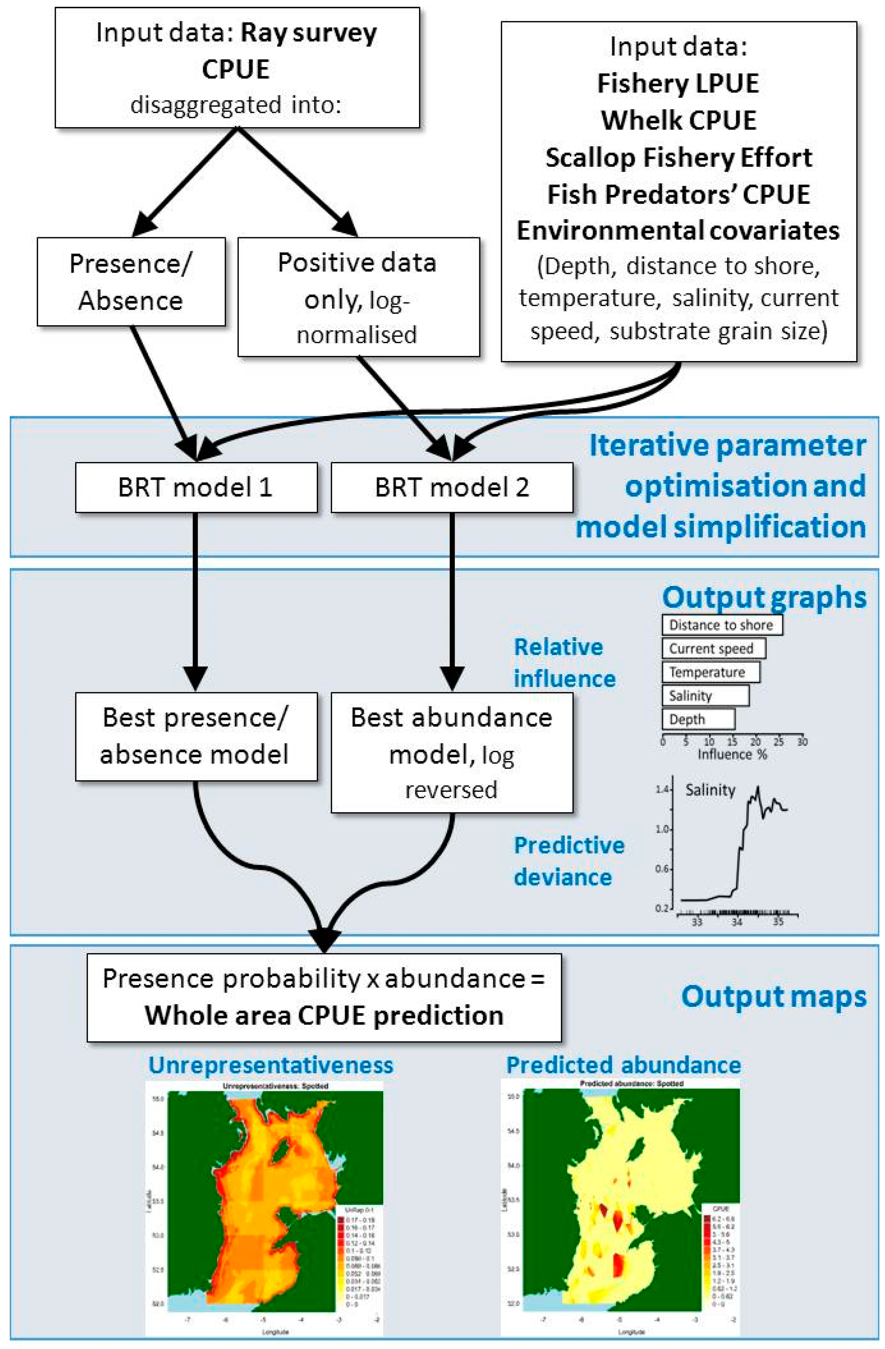
Delta log-normal boosted regression trees split zero-inflated, long-tailed distribution data (most trawls caught nothing, and very few caught many specimens) into zero/non-zero catches, converted to 0 or 1, and log-normalized non-zero catches (CPUE) (see Figure 5, [11] and [28] for a more detailed explanation).
The model used the author’s own function gbm.auto [60] with the following BRT parameter values:
- Tree complexity, controlling variable interactions, of 2 or 15 for all juveniles, 2 or 6 for all mature females (whelk, scallop, and fish predators are not included in the female model). This allows us to evaluate whether all variables interacting provides a better model result than only two.
- Learning rate, controlling the contribution each tree has to the model, of 0.01 and 0.005 for all rays bar mature female blonde rays where we used 0.01 and 0.001 as this subset has fewer data. Smaller rates processing slower but usually more accurately.
The model loops through all combinations of these parameters to find the best one, then tests whether that combination would perform better with any variables omitted (using the gbm.simplify function). The best combination is chosen based on performance metrics generated by the model, such as the training data correlation (the correlation between the whole dataset split into training and testing data; higher is better) and mean deviance (lower is better). Performance of the best binary models was quantified using the AUC statistic [61], calculated for the training and CV data used in the model. The discrepancy between the two indicates overfitting, which BRT modeling is designed to reduce with the k-fold (10) CV subroutine. Model validation is conducted by testing the predictive performance of the training-learnt BRT model object (the size of which is determined by the Bag Fraction) against the (remaining) testing data, before all data are used to construct the final model object which is used for prediction [28].
The model machine-learns the relationship between the explanatory variables and each of the two split sets of response variables. Probability of occurrence is predicted using a BRT model with a binomial distribution on the zero/non-zero catches, then abundance is predicted using a BRT model on the non-zero catches with a Gaussian distribution (under the assumption of normally distributed data once the zero-inflated and long tailed elements are accounted for). Predicted abundance values are then inverse log transformed and bias-corrected to avoid inaccuracies associated with using exponents [62]. The probability of occurrence is then multiplied by expected abundance to create predicted CPUE values for the whole study area, exported as csv files and maps. Bar plots of the most influential variables are created, as are partial dependence plots resulting from thousands of binary predictive splits whereby the model learns a more nuanced predictor/response relationship for each variable—for more see [11].
4.1. Database Selection and Processing
The substrate of the Irish Sea is mostly a sandy/gravel mix, generally finer close to shore, with rocks to the center/Eastern edges (off Anglesey) and a large mud bank along the Western edge (Dublin coast), with lower current speed there. Current speed at the bottom is low to moderate other than at a few headlands [63]. It is a well-mixed sea but a persistent front develops in the summer. The Irish Sea is a shallow-shelf sea with a 100 m-deep Central Channel and very shallow (≤5 m) sandbanks running along the Western edge (Irish coast), which create deeper channels 7–12 km from shore [24,63,64].
4.1.1. Environmental Covariates
Surveyed CPUE of rays in the Irish Sea show correlations with depth, substrate, temperature, salinity, current speed and distance to shore [11,38,68,69]. Neither standard linear correlations nor GAMs (conducted on these data in previous studies [11]) revealed stronger relationships between survey CPUE and any specific month of environmental variable data. Since the survey trawls were conducted in September, environmental data from September were used in this analysis. Correlated variables can be problematic for some modeling techniques, however unlike GLMs or simple regression trees, BRTs are robust to auto-correlated variables as they feature mechanisms (regularization and stochasticity processes [28]), which improves (minimizes) their overfitting [20,52,70]. [28] also find that overfitting does not compromise BRT predictions. Nonetheless, linear correlations between environmental variable pairs did not exceed an r² value of 0.37, and were generally 0.14 or below, limiting cause for concern.
4.1.2. Fishery LPUE
Including fishing pressure might improve predicted ray distributions, so ray LPUE data from demersal trawls operating in the Irish Sea were used as an explanatory variable for the juveniles and mature female CPUE analysis. These data were averaged across the available time period (2006–2012) [9].
4.1.3. Whelk CPUE and Scallop Fishery Effort
Similarly, including processes that remove egg cases might improve predicted distributions of juvenile ray CPUEs. These species deposit fertilized eggs on the seabed, which may be removed by humans or natural predators. Scallop dredging occurs in the Irish Sea on sand and gravel [71,72,73], where rays can lay eggs, which scallop dredges are known to remove [74,75], so higher dredging effort should remove more eggcases. Scallop effort data were then binned into ICES rectangles and averaged across all available years. Whelks (Buccinum undatum) are strongly implicated in the predation of elasmobranch eggcases [76,77,78]. High surveyed whelk LPUE likely indicates high abundance and thus higher eggcases predation. Whelk LPUE data were binned into ICES rectangles and averaged across all available years.
4.1.4. Fish Predators’ CPUE
To obtain the CPUE of potential predator species at the size range where they could potentially prey on newborn rays, we first needed to compute the size ranges of those species. The weight of an individual marine predator is generally about 100 times the weight of their prey items, plus or minus one order of magnitude [79]. Therefore, potential ray predators would be at least ten times the rays’ birth weight. To calculate this, lengths at birth from [80] were converted to weights using equation W = a x Lb, where a and b are constants again from [80]. The weights were multiplied by ten (100 minus one order of magnitude), then converted back to lengths using the inverse of the previous equation, using predator-specific a and b values from [81], i.e., . The resultant lengths are the hypothesised minimum sizes of the potential predatory species of age 0 rays. These sizes were used to filter the survey data for each combination of the four ray species and six potential fish predator species (five for blonde rays). Potential predators (“surveyed fish predator CPUE” in Table 3) were cod (Gadus morhua), haddock (Melanogrammus aeglefinus), plaice (Pleuronectes platessa), whiting (Merlangius merlangus), common skate (Dipturus flossada) and blonde ray (treated as a potential predator for all but blonde ray since these species spatially segregate by size to avoid cannibalism [82]). These species were chosen as a representative selection of the more common piscivores in the Irish Sea, since some of these and similar species have been recorded predating upon these young rays/eggcases in the Irish Sea and surrounding waters [35].
4.1.5. Ray Survey CPUE
Ray survey CPUE data were pooled across all available years as there were insufficient data in any one year for the model to run. Trawl midpoints were used as catch locations, many of which overlapped as the survey aims to resample sites in successive years (see Section 2.2). For the mature female analysis, data were limited to females at or above total length at first maturity—49 cm for cuckoo ray, 60 for thornback, 81 for blonde, and 52 for spotted ray [49,83]. For juvenile analysis, data were limited to rays ≤34/33/36/33 cm (respectively): the maximum lengths at age 1 calculated using the growth parameters of [80].
In order to create a single database of explanatory variables to be predicted to, explanatory variables were interpolated to the highest resolution dataset, which was depth points covering the whole Irish Sea. Distance to shore was calculated using raster proximity analysis in QGIS mapping software [84]. The substrate layer was converted from descriptive Folk classifications [85] into median grain size [86], allowing it to be treated as a continuous variable by the model. For the gridded data where the model predicts CPUE values, polygon layers (ray and whelk trawl catch rates, scallop effort) were appended to the depth points directly, while point layers were first converted to Voronoi polygons then appended. For the response variable dataset, explanatory variables were appended to the ray survey data points using the same approach.
4.2. Preliminary Analysis
Compared to the whole study area, the survey trawls under-sample extreme shallows, depths over 50 m, corresponding distances from shore (close and far, respectively), and areas of high current velocity [11]. This was not considered an issue as the model compares sampling frequency of variable ranges from the survey, to the whole study area, and produces “unrepresentativeness maps” using our RSB function (gbm.rsb) in R [87]. These describe the extent to which environmental conditions (depth, current speed etc.) across the study area are represented by the range of conditions encountered in the sampling survey and allows the user to assign a level of confidence to the outputs (Figure S1).
Auto-correlation of sample data locations (all trawls) was checked to ensure that neighboring points were statistically independent [88,89] by analyzing the residuals of a GAM of CPUE as explained by latitude and longitude, which showed the residuals to be normally distributed (mgcv in R). A Mantel test (vegan in R) showed the model sufficiently accounted for spatial autocorrelation in the raw data, and that the residuals were not auto-correlated (Mantel correlation 0.078, p = 0.001) [89,90].
4.3. Modelling Approach
For the juvenile subset, the model was run twice for each species. Once with all six (five for blonde ray) fish predator CPUEs as individual variables, and then with those CPUEs combined. Based on performance metrics, individual variables outperformed combined variables in seven of the eight comparisons (four species’ binary and Gaussian BRTs). This makes sense as BRTs can accommodate numerous explanatory variables without penalty [20,28]. We therefore kept variables separate.
To examine the relative importance of each variable in the model, the percentage influence values displayed on the bar plots of variable influence (top left panes in Figure S2a–i) were totaled for each individual variable and grouped into categories: environmental (temperature, salinity, distance to shore, current speed, depth, substrate grain size), fishery (fishery CPUE), potential fish predators (cod, haddock, plaice, whiting, common skate, blonde ray) and eggcase removers (whelk LPUE, scallop effort). This was done for the binary and Gaussian models, for each species (Figure 1).
Amalgamated predicted CPUE maps were initially created by adding the adult and juvenile maps’ values together. Maximum CPUE was highest for spotted ray (8.9 fish per hour total; 8.1 for juveniles and 1.1 for mature females) and lowest for blonde ray (1.1 fish per hour total; 0.87 juveniles, 0.56 mature females). To avoid the most abundant subset (juvenile spotted rays) dominating the combined CPUE, we normalized both of the original maps’ ranges to 1, then summed them to give a theoretical maximum of 2, presented as a percentage for ease of interpretation (Figure 3). A similar process was used for Figure 4: each species’ dataset for juveniles and adult females were scaled to 1 and summed to a total of 8, again presented as a percentage.
5. Conclusions
The study has shown that the distribution of mature female and juvenile rays in the Irish Sea can be predicted using an appropriate choice of covariates and available survey data. The analysis method chosen, Boosted Regression Trees, allowed us to model these distributions with many different covariates, but without over-fitting, a common problem with advanced regression methods. Differences in response and hence distribution between adult females and juveniles were also revealed by the use of population component subsets, opening up novel possibilities for nuanced spatial management to protect spawning and nursery areas; these analyses also improved the predictive power of the models. Normalizing and combining their maps into a single map makes the results of these analyses more accessible to users and managers, with the underlying code facilitating rapid processing of these outputs.
Supplementary Materials
The following are available online at https://www.mdpi.com/2410-3888/2/3/12/s1, Figure S1: RSB map of mature female and juvenile cuckoo, thornback, blonde and spotted rays. The product of comparing histograms of each explanatory variable’s values at the response variable sampling sites, with the histograms of those explanatory variables across the whole study area. The modulus of the differences for each histogram bar region, for each variable, for both binary and Gaussian maps, are added, resulting in maps where higher numbers indicate higher total deviance from a representative coverage of the explanatory variable values at that site. These maps give a spatial representation of how well those bins of the environmental variables at a specific site (e.g., 20 m depth, 3 km from shore) are represented in the samples data, i.e., how much confidence one can have for abundance predictions at that site; Figures S2a–i: Bar plots of the relative influence of each explanatory variable to the predicted abundance maps of each species, showing which are the most important, and “partial dependence” line plots detailing the relationship of those variables to predicted ray CPUE. Only produced for Gaussian bars and partial dependence lines, as both binary and Gaussian lines tend to be similar, and only produced for variables exerting >5% influence, in order to reduce figure numbers from 180 to 62.
Acknowledgments
The authors appreciate the data provided by Hans Gerritsen and his assistance with interpreting the Marine Institute and DATRAS data. We gratefully acknowledge the critical comments of the reviewers, which helped to improve the manuscript. Research funding was received from the European Community’s Seventh Framework Programme (FP7/2007–2013) under grant agreement MYFISH number 289257. David G. Reid also acknowledges funding from a Beaufort Marine Research Award, carried out under the Sea Change Strategy and the Strategy for Science Technology and Innovation (2006–2013), with the support of the Marine Institute, funded under the Marine Research Sub-Programme of the National Development Plan 2007–2013. The funders had no role in study design, data collection and analysis, decision to publish, or preparation of the manuscript.
Author Contributions
Conceived and designed analyses: S.D., D.B., R.O., D.G.R. and M.J.C. Performed analyses: S.D. Wrote paper: S.D., D.B., R.O., D.G.R. and M.J.C.
Conflicts of Interest
The authors declare no conflict of interest. The founding sponsors had no role in the design of the study; in the collection, analyses, or interpretation of data; in the writing of the manuscript, and in the decision to publish the results.
Appendix A
R functions and packages used
- dismo: Hijmans, R.L., Phillips, S., Leathwick, J. and Elith, J. 2103. dismo: Functions for species distribution modelling, that is, predicting entire geographic distributions from occurrences at a number of sites. R package version: 0.9-3. http://cran.r-project.org/package=dismo
- gam: Hastie, T. 2013. gam: Generalized Additive Models. R package version 1.09. http://CRAN.R-project.org/package=gam
- gbm: Ridgeway, G. 2013. gbm: Generalised Boosted Regression Models. R package version: 2.1. http://cran.r-project.org/package=gbm
- mapplots: Gerritsen, H. 2014. mapplots: Data Visualisation on Maps. R package version 1.5. http://CRAN.R-project.org/package=mapplots
- mgcv: Wood, S.N. 2011. Mgcv: Fast stable restricted maximum likelihood and marginal likelihood estimation of semiparametric generalized linear models. Journal of the Royal Statistical Society (B) 73(1):3-36. http://CRAN.R-project.org/package=mgcv
- vegan: Oksanen, J., Blanchet, F.G., Kindt, R., Legendre, P., Minchin, P.R., O’Hara, R.B., Simpson, G.L., Solymos, P., Stevens, M.H.H. and Wagner, H. 2013. vegan: Community Ecology Package. R package version 2.0-10. http://CRAN.R-project.org/package=vegan
- R package functions gbm.auto, including gbm.map, gbm.rsb, gbm.cons, gbm.valuemap and gbm.bfcheck, written by SD 2012-2016 and available at: https://github.com/SimonDedman/gbm.auto
References
- Rogers, S.; Ellis, J.R. Changes in the demersal fish assemblages of British coastal waters during the 20th century. ICES J. Mar. Sci. 2000, 57, 866–881. [Google Scholar] [CrossRef]
- Ellis, J.R.; Clarke, M.W.; Cortés, E.; Heessen, H.J.; Apostolaki, P.; Carlson, J.K.; Kulla, D.W. Management of elasmobranch fisheries in the North Atlantic. Adv. Fish. Sci. 2008, 50, 184–228. [Google Scholar]
- Walker, P.; Heessen, H. Long-term changes in ray populations in the North Sea. ICES J. Mar. Sci. 1996, 53, 1085–1093. [Google Scholar] [CrossRef]
- Baum, J.K.; Myers, R.A.; Kehler, D.G.; Worm, B.; Harley, S.J.; Doherty, P.A. Collapse and conservation of shark populations in the Northwest Atlantic. Science 2003, 299, 389–392. [Google Scholar] [CrossRef] [PubMed]
- Ellis, J.R.; Dulvy, N.K.; Jennings, S.; Parker-Humphreys, M.; Rogers, S.I. Assessing the status of demersal elasmobranchs in UK waters: A review. J. Mar. Biol. Assoc. UK 2005, 85, 1025–1048. [Google Scholar] [CrossRef]
- Worm, B.; Davis, B.; Kettemer, L.; Ward-Paige, C.A.; Chapman, D.; Heithaus, M.R.; Kessel, S.T.; Gruber, S.H. Global catches, exploitation rates, and rebuilding options for sharks. Mar. Policy 2013, 40, 194–204. [Google Scholar] [CrossRef]
- Brander, K. Disappearance of common skate Raia batis from Irish Sea. Nature 1981, 290, 48–49. [Google Scholar] [CrossRef]
- Walker, P.; Hislop, J. Sensitive skates or resilient rays? Spatial and temporal shifts in ray species composition in the central and north-western North Sea between 1930 and the present day. ICES J. Mar. Sci. 1998, 55, 392–402. [Google Scholar] [CrossRef]
- Marine Institute. The Stock Book 2014; Marine Institute: Galway, Ireland, 2014. [Google Scholar]
- International Council for the Exploration of the Sea. Manual for the international bottom trawl surveys in the western and southern areas. In Proceedings of the International Bottom Trawl Survey Working Group, Lisbon, Portugal, 22–26 March 2010. [Google Scholar]
- Dedman, S.; Officer, R.; Brophy, D.; Clarke, M.W.; Reid, D.G. Modelling abundance hotspots for data-poor Irish sea rays. Ecol. Model. 2015, 312, 77–90. [Google Scholar] [CrossRef]
- European Union. Council Regulation (EU) No 2016/72 of 22 January 2016 Fixing for 2016 the Fishing Opportunities for Certain Fish Stocks and Groups of Fish Stocks, Applicable in Union Waters and, to Union Vessels, in Certain Non-Union waters, and Amending Regulation (EU) 2015/104. Off. J. Eur. Union 2016, 22, 1–165. [Google Scholar]
- North Western Waters Advisory Council. Shark Ray Skate Focus Group Report; North Western Waters Advisory Council: Dublin, Ireland, 2012. [Google Scholar]
- European Commission. No. 1380/2013 of the European Parliament and of the Council of 11 December 2013 on the Common Fisheries Policy, amending Council Regulations (EC) No 1954/2003 and (EC) No 1224/2009 and repealing Council Regulations (EC) No 2371/2002 and (EC) No 639/2004 and Council Decision 2004/585/EC. Off. J. Eur. Union 2013, 354, 22–61. [Google Scholar]
- International Council for the Exploration of the Sea Working Group on Elasmobranch Fishes (ICES WGEF). Report of the Working Group on Elasmobranch Fishes (WGEF); International Council for the Exploration of the Sea Working Group on Elasmobranch Fishes: Lisbon, Portugal, 2012. [Google Scholar]
- International Council for the Exploration of the Sea Working Group on Elasmobranch Fishes (ICES WGEF). Report of the Working Group on Elasmobranch Fishes (WGEF); International Council for the Exploration of the Sea Working Group on Elasmobranch Fishes: Lisbon, Portugal, 2015. [Google Scholar]
- International Council for the Exploration of the Sea Working Group on Elasmobranch Fishes (ICES WGEF). ICES Advice: Rays and skates in Subarea VI and Divisions VIIa–c, e–j (Celtic Sea and west of Scotland); International Council for the Exploration of the Sea Working Group on Elasmobranch Fishes: Lisbon, Portugal, 2012. [Google Scholar]
- Edgar, G.J.; Stuart-Smith, R.D.; Willis, T.J.; Kininmonth, S.; Baker, S.C.; Banks, S.; Barrett, N.S.; Becerro, M.A.; Bernard, A.T.F.; Berkhout, J.; et al. Global conservation outcomes depend on marine protected areas with five key features. Nature 2014, 506, 216–228. [Google Scholar] [CrossRef] [PubMed] [Green Version]
- Ellis, J.R.; Silva, J.F.; McCully, S.R.; Evans, M.; Catchpole, T. UK Fisheries for Skates (Rajidae): History and Development of the Fishery, Recent Management Actions and Survivorship of Discards; International Council for the Exploration of the Sea: Lisbon, Portugal, 2010. [Google Scholar]
- Abeare, S.M. Comparisons of Boosted Regression Tree, GLM and GAM Performance in the Standardization of Yellowfin Tuna Catch-Rate Data from the Gulf of Mexico Longline Fishery. Ph.D. Thesis, University of Pretoria, Gauteng, South Africa, 2009. [Google Scholar]
- Lo, N.C.; Jacobson, L.D.; Squire, J.L. Indices of relative abundance from fish spotter data based on delta-lognormal models. Can. J. Fish. Aquat. Sci. 1992, 49, 2515–2526. [Google Scholar] [CrossRef]
- De Raedemaecker, F.; Brophy, D.; O’Connor, I.; Comerford, S. Habitat characteristics promoting high density and condition of juvenile flatfish at nursery grounds on the west coast of Ireland. J. Sea Res. 2012, 73, 7–17. [Google Scholar] [CrossRef]
- Ball, I.R.; Possingham, H.P. MARXAN—A Reserve System Selection Tool. 2013. Available online: http://www.ecology.uq.edu.au/marxan.htm (accessed on 13 June 2013).
- Vincent, M.A.; Atkins, S.M.; Lumb, C.M.; Golding, N.; Lieberknecht, L.M.; Webster, M. Marine Nature Conservation and Sustainable Development—The Irish Sea Pilot; Joint Nature Conservation Committee: Peterborough, UK, 2004. [Google Scholar]
- Loos, S.A. Exploration of MARXAN for Utility in Marine Protected Area Zoning. Master’s Thesis, University of Victoria, Victoria, BC, Canada, 2006. [Google Scholar]
- Elith, J.; Phillips, S.J.; Hastie, T.; Dudík, M.; Chee, Y.E.; Yates, C.J. A statistical explanation of MaxEnt for ecologists. Divers. Distrib. 2011, 17, 43–57. [Google Scholar] [CrossRef]
- Phillips, S.J.; Dudík, M.; Schapire, R.E. A maximum entropy approach to species distribution modeling. In Proceedings of the Twenty-First International Conference on Machine Learning, Banff, Canada, July 2004; pp. 655–662. [Google Scholar]
- Elith, J.; Leathwick, J.R.; Hastie, T. A working guide to boosted regression trees. J. Anim. Ecol. 2008, 77, 802–813. [Google Scholar] [CrossRef] [PubMed]
- Johnston, G.; Tetard, A.; Santos, A.R.; Kelly, E.; Clarke, M.W. Spawning and Nursery Areas of Selected Rays and Skate Species in the Celtic Seas; Marine Institute: Galway, Ireland, 2014. [Google Scholar]
- Hijmans, R.J.; Elith, J. Species Distribution Modeling with R, R package version 08-11; 2013. [Google Scholar]
- Froeschke, J.; Drymon, M. Atlantic Sharpnose Shark: Standardized Index of Relative Abundance Using Boosted Regression Trees and Generalized Linear Models; SEDAR34-WP-12; SEDAR: North Charleston, SC, USA, 2013; 31p. [Google Scholar]
- Lane, J.Q.; Raimondi, P.T.; Kudela, R.M. Development of a logistic regression model for the prediction of toxigenic Pseudo-nitzschia blooms in Monterey Bay, California. Mar. Ecol. Prog. Ser. 2009, 383, 37–51. [Google Scholar] [CrossRef]
- Bergmann, M.; Hinz, H.; Blyth, R.; Kaiser, M.; Rogers, S.; Amrstrong, M. Using knowledge from fishers and fisheries scientists to identify possible groundfish “Essential Fish Habitats”. Fish. Res. 2004, 66, 373–379. [Google Scholar] [CrossRef]
- Frank, K.T.; Petrie, B.; Shackell, N.L. The ups and downs of trophic control in continental shelf ecosystems. Trends Ecol. Evol. 2007, 22, 236–242. [Google Scholar] [CrossRef] [PubMed]
- Pinnegar, J.K. DAPSTOM—An Integrated Database & Portal for Fish Stomach Records; Centre for Environment, Fisheries & Aquaculture Science: Lowestoft, UK, 2014. [Google Scholar]
- Shephard, S.; Gerritsen, H.; Kaiser, M.J.; Reid, D.G. Spatial heterogeneity in fishing creates de facto refugia for endangered celtic sea elasmobranchs. PLoS ONE 2012, 7, e49307. [Google Scholar] [CrossRef] [PubMed]
- Rogers, S.I.; Maxwell, D.; Rijnsdorp, A.D.; Damm, U.; Vanhee, W. Fishing effects in northeast Atlantic shelf seas: Patterns in fishing effort, diversity and community structure. IV. Can comparisons of species diversity be used to assess human impacts on demersal fish faunas? Fish. Res. 1999, 40, 135–152. [Google Scholar] [CrossRef]
- Kaiser, M.; Bergmann, M.; Hinz, H.; Galanidi, M.; Shucksmith, R.; Rees, E.I.S.; Darbyshire, T.; Ramsay, K. Demersal fish and epifauna associated with sandbank habitats. Estuar. Coast. Shelf Sci. 2004, 60, 445–456. [Google Scholar] [CrossRef]
- Shelmerdine, R.L.; Stone, D.; Leslie, B.; Robinson, M. Implications of defining fisheries closed areas based on predicted habitats in Shetland: A proactive and precautionary approach. Mar. Policy 2013, 43, 184–199. [Google Scholar] [CrossRef]
- Murphy, H.M.; Jenkins, G.P. Observational methods used in marine spatial monitoring of fishes and associated habitats: A review. Mar. Freshwater Res. 2010, 61, 236–252. [Google Scholar] [CrossRef]
- Brown, K.; Adger, W.N.; Tompkins, E.; Bacon, P.; Shim, D.; Young, K. Trade-off analysis for marine protected area management. Ecol. Econ. 2001, 37, 417–434. [Google Scholar] [CrossRef]
- International Council for the Exploration of the Sea Working Group on Elasmobranch Fishes (ICES WGEF). Report of the Working Group on Elasmobranch Fishes (WGEF); International Council for the Exploration of the Sea Working Group on Elasmobranch Fishes: Lisbon, Portugal, 2014. [Google Scholar]
- Heupel, M.R.; Carlson, J.K.; Simpfendorfer, C.A. Shark nursery areas: Concepts, definition, characterization and assumptions. Mar. Ecol. Prog. Ser. 2007, 337, 287–297. [Google Scholar] [CrossRef]
- Queirós, A.M.; Huebert, K.B.; Keyl, F.; Fernandes, J.A.; Stolte, W.; Maar, M.; Kay, S.; Jones, M.C.; Hamon, K.G.; Hendriksen, G.; et al. Solutions for ecosystem-level protection of ocean systems under climate change. Glob. Chang. Biol. 2016, 22, 3927–3936. [Google Scholar] [CrossRef] [PubMed]
- Maia, C.; Erzini, K.; Serra-Pereira, B.; Figueiredo, I. Reproductive biology of cuckoo ray Leucoraja naevus. J. Fish Biol. 2012, 81, 1285–1296. [Google Scholar] [CrossRef] [PubMed]
- Clark, R.S. Rays and Skates (Raiæ) No. 1.—Egg-Capsules and Young. J. Mar. Biol. Assoc. 1922, 12, 578–643. [Google Scholar] [CrossRef]
- Holden, M. The fecundity of Raja clavata in British waters. ICES J. Mar. Sci. 1975, 36, 110–118. [Google Scholar] [CrossRef]
- Steven, G. Migrations and growth of the thornback ray. J. Mar. Biol. Assoc. 1936, 20, 605–614. [Google Scholar] [CrossRef]
- Ryland, J.; Ajayi, T. Growth and population dynamics of three Raja species (Batoidei) in Carmarthen Bay, British Isles. ICES J. Mar. Sci. 1984, 41, 111–120. [Google Scholar] [CrossRef]
- Walker, P.; Ellis, J.R. Ecology of rays of the north-eastern Atlantic. In Biology of Skates, Proceedings of the Biology of Skates Symposium (New Orleans, 1996); Princeton Press: New Orleans, LA, USA, 1998; pp. 7–29. [Google Scholar]
- Knudby, A.; LeDrew, E.; Brenning, A. Predictive mapping of reef fish species richness, diversity and biomass in Zanzibar using IKONOS imagery and machine-learning techniques. Remote Sens. Environ. 2010, 114, 1230–1241. [Google Scholar] [CrossRef]
- Elith, J.; Graham, C.H.; Anderson, R.P.; Dudík, M.; Ferrier, S.; Guisan, A.; Hijmans, R.J.; Huettmann, F.; Leathwick, J.R.; Lehmann, A.; et al. Novel methods improve prediction of species’ distributions from occurrence data. Ecography 2006, 29, 129–151. [Google Scholar] [CrossRef]
- Agardy, T.; Di Sciara, G.N.; Christie, P. Mind the gap: Addressing the shortcomings of marine protected areas through large scale marine spatial planning. Mar. Policy 2011, 35, 226–232. [Google Scholar] [CrossRef]
- Buxton, C.; Barrett, N.; Haddon, M.; Gardner, C.; Edgar, G. Evaluating the Effectiveness of Marine Protected Areas as a Fisheries Management Tool; Tasmanian Aquaculture and Fisheries Institute: Hobart, Tasmania, 2006. [Google Scholar]
- Rhodes, J.R.; Callaghan, J.G.; McAlpine, C.A.; de Jong, C.; Bowen, M.E.; Mitchell, D.; Lunney, D.; Possingham, H.P. Regional variation in habitat-occupancy thresholds: A warning for conservation planning. J. Appl. Ecol. 2008, 45, 549–557. [Google Scholar] [CrossRef]
- Dedman, S.; Officer, R.; Brophy, D.; Clarke, M.W.; Reid, D.G. Towards a flexible Decision Support Tool for MSY-based Marine Protected Area design for skates and rays. ICES J. Mar. Sci. 2017, 74, 576–587. [Google Scholar] [CrossRef]
- Klein, C.J.; Tulloch, V.J.; Halpern, B.S.; Selkoe, K.A.; Watts, M.E.; Steinback, C.; Scholz, A.; Possingham, H.P. Tradeoffs in marine reserve design: Habitat condition, representation, and socioeconomic costs. Conserv. Lett. 2013, 6, 324–332. [Google Scholar] [CrossRef]
- Penn, J.W.; Fletcher, W.J. The Efficacy of Sanctuary Areas for the Management of Fish Stocks and Biodiversity in WA Waters; Government of Western Australia Department of Fisheries: North Beach, Western Australia, Australia, 2010.
- Little, A.S.; Needle, C.L.; Hilborn, R.; Holland, D.S.; Marshall, C.T. Real-time spatial management approaches to reduce bycatch and discards: Experiences from Europe and the United States. Fish Fish. 2014. [Google Scholar] [CrossRef]
- Dedman, S.; Officer, R.; Brophy, D.; Clarke, M.W.; Reid, D.G. Gbm.auto: Automated delta log-normal boosted regression tree spatial modelling and MPA generation in R. PLoS ONE 2017. (In Press) [Google Scholar]
- Parisien, M.-A.; Moritz, M. Environmental controls on the distribution of wildfire at multiple spatial scales. Ecol. Monogr. 2009, 79, 127–154. [Google Scholar] [CrossRef]
- Duan, N. Smearing estimate: A nonparametric retransformation method. J. Am. Stat. Assoc. 1983, 78, 605–610. [Google Scholar] [CrossRef]
- Connor, D.W.; Gilliland, P.M.; Golding, N.; Robinson, P.; Tod, D.; Verling, E. UKSeaMap: The Mapping of Seabed and Water Column Features of UK Seas; JNCC, Ed.; Joint Nature Conservation Committee: Peterborough, UK, 2006. [Google Scholar]
- Boelens, R.; Maloney, D.; Parsons, A.; Walsh, A. Ireland’s Marine and Coastal Areas and Adjacent Seas: An Environmental Assessment; Boelens, R.G.V., Maloney, D.M., Parsons, A.P., Walsh, A.R., Eds.; Marine Institute: Dublin, Ireland, 1999. [Google Scholar]
- EMODnet. EMODnet Biological Data Products. 2014. Available online: http://bio.emodnet.eu (accessed on 14 November 2012).
- British Geological Survey. Digital Geological Map of Great Britain’s Sea Bed Sediments 1:250,000 Scale (DiGSBS250K) Data [CD-ROM], 3rd ed.; British Geological Survey: Nottingham, UK, 2011. [Google Scholar]
- ICES. ICES Database of Trawl Surveys 1990–2014. 2015. Available online: http://datras.ices.dk (accessed on 13 February 2015).
- Martin, C.; Vaz, S.; Ellis, J.R.; Lauria, V.; Coppin, F.; Carpentier, A. Modelled distributions of ten demersal elasmobranchs of the eastern English Channel in relation to the environment. J. Exp. Mar. Biol. Ecol. 2012, 418, 91–103. [Google Scholar] [CrossRef]
- Ellis, J.R.; Cruz-Martinez, A.; Rackham, B.; Rogers, S. The distribution of chondrichthyan fishes around the British Isles and implications for conservation. J. Northwest Atl. Fish. Sci. 2005, 35, 195–213. [Google Scholar] [CrossRef]
- Potts, J.M.; Elith, J. Comparing species abundance models. Ecol. Model. 2006, 199, 153–163. [Google Scholar] [CrossRef]
- Minchin, D. Biological observations on young scallops, Pecten maximus. J. Mar. Biol. Assoc. UK 1992, 72, 807–819. [Google Scholar] [CrossRef]
- Paul, J.D. Natural settlement and early growth of spat of the queen scallop Chlamys opercularis (L.), with reference to the formation of the first growth ring. J. Molluscan Stud. 1981, 47, 53–58. [Google Scholar] [CrossRef]
- Eggleston, D. Spat of the scallop (Pecten maximus (L.)) from off Port Erin, Isle of Man. Rep. Mar. Biol. Stn. Port Erin 1962, 74, 29–32. [Google Scholar]
- North Pacific Fishery Management Council (NPFMC) and NMFS. Final Environmental Assessment for Amendment 104 to the Fishery Management Plan for Groundfish of the Bering Sea and Aleutian Islands Management Area: Habitat Areas of Particular Concern (HAPC) Areas of Skate Egg Concentration; North Pacific Fishery Management Council and NMFS: Anchorage, AK, USA, 2014. [Google Scholar]
- Hitz, C.R. Observations on egg cases of the big skate (Raja binoculata Girard) found in Oregon coastal waters. J. Fish. Board Can. 1964, 21, 851–854. [Google Scholar] [CrossRef]
- Cox, D.L.; Koob, T.J. Predation on elasmobranch eggs. Environ. Biol. Fish. 1993, 38, 117–125. [Google Scholar] [CrossRef]
- Cox, D.L.; Walker, P.; Koob, T.J. Predation on eggs of the thorny skate. Trans. Am. Fish. Soc. 1999, 128, 380–384. [Google Scholar] [CrossRef]
- Kabat, A.R. Predatory ecology of naticid gastropods with a review of shell boring predation. Malacol. Int. J. Malacol. 1990, 32, 155–193. [Google Scholar]
- Nakazawa, T.; Ushio, M.; Kondoh, M. Scale dependence of predator-prey mass ratio: Determinants and applications. In Advances in Ecological Research; Belgrano, A., Reiss, J., Eds.; Academic Press: Amsterdam, The Netherlands, 2011; Volume 45, pp. 269–302. [Google Scholar]
- Gallagher, M.J. The Fisheries Biology of Commercial Ray Species from Two Geographically Distinct Regions. Ph.D. Thesis, University of Dublin, Dublin, Ireland, 2000. [Google Scholar]
- Coull, K.; Jermyn, A.; Newton, A.; Henderson, G.; Hall, W. Length/Weight Relationships for 88 Species of Fish Encountered in the North East Atlantic; Department of Agriculture and Fisheries for Scotland Marine Laboratory: Aberdeen, UK, 1989. [Google Scholar]
- Compagno, L.J.V. Alternative Life-History Styles of Cartilaginous Fishes in Time and Space. Alternative Life-History Styles of Fishes; Springer: Dordrecht, The Netherlands, 1990; Volume 28, pp. 33–75. [Google Scholar]
- McCully, S.R.; Scott, F.; Ellis, J.R. Lengths at maturity and conversion factors for skates (Rajidae) around the British Isles, with an analysis of data in the literature. ICES J. Mar. Sci. 2012, 69, 1812–1822. [Google Scholar] [CrossRef]
- Quantum GIS Development Team. Quantum GIS Geographic Information System, v2.14.5. 2014. Available online: http://qgis.osgeo.org (accessed on 1 August 2017).
- Folk, R.L. The distinction between grain size and mineral composition in sedimentary-rock nomenclature. J. Geol. 1954, 62, 344–359. [Google Scholar] [CrossRef]
- SearchMESH. Median Grain Size Chart. 2014. Available online: http://www.searchmesh.net/images/gmhm2-38_table-sediment_classifications.jpg (accessed on 13 June 2014).
- R Core Team. R: A Language and Environment for Statistical Computing. R Foundation for Statistical Computing, v3.4.1. 2013. Available online: www.R-project.org (accessed on 1 August 2017).
- Miller, J.A. Species distribution models: Spatial autocorrelation and non-stationarity. Prog. Phys. Geogr. 2012, 36, 681–692. [Google Scholar] [CrossRef]
- Redfern, J.V.; Ferguson, M.C.; Becker, E.A.; Hyrenbach, K.D.; Good, C.; Barlow, J.; Kaschner, K.; Baumgartner, M.F.; Forney, K.A.; Balance, L.T.; et al. Techniques for cetacean-habitat modeling. Mar. Ecol. Prog. Ser. 2006, 310, 271–295. [Google Scholar] [CrossRef]
- Dormann, F.C.; McPherson, M.J.; Araújo, B.M.; Bivand, R.; Bolliger, J.; Gudrun, C.; Richard, G.D.; Alexandre, H.; Walter, J.; Kissling, W.D.; et al. Methods to account for spatial autocorrelation in the analysis of species distributional data: A review. Ecography 2007, 30, 609–628. [Google Scholar] [CrossRef]
- Friedman, J.H. Greedy function approximation: A gradient boosting machine. Ann. Stat. 2001, 29, 1189–1232. [Google Scholar] [CrossRef]
Figure 1.
Average influence of grouped explanatory variable types, on mature female (top 5 rows; row 1 is mature female average) and juvenile (bottom 5 rows; sixth row is juvenile average) surveyed ray binary presence/absence plus Gaussian Catch Per Unit Effort (CPUE). Input data are the binary and Gaussian bar plot figures reproduced in Figure S2a–i.
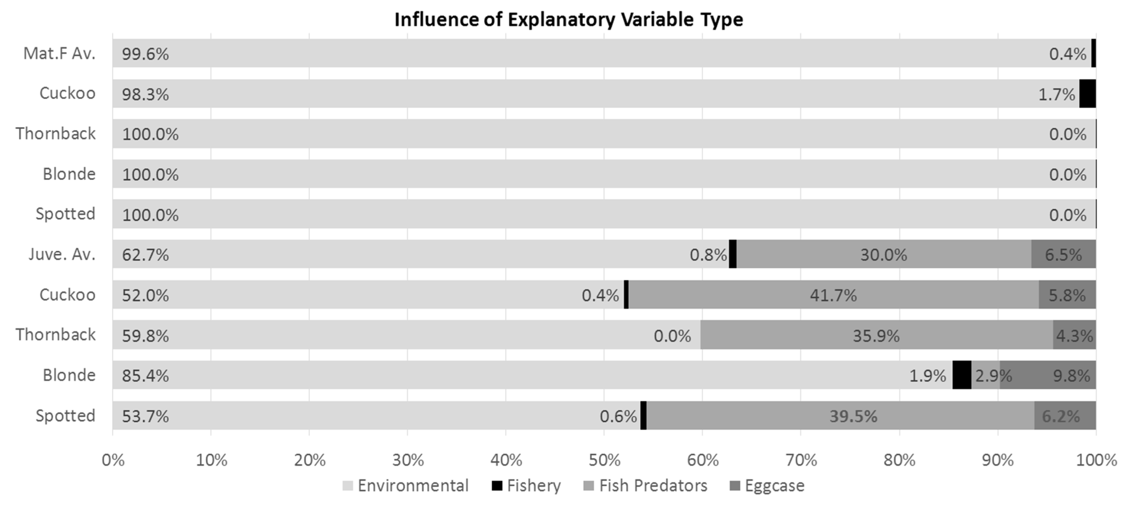
Figure 2.
Model predicted CPUE (numbers per hour) of mature female rays based on environmental variables and fishing pressure (left column) and juvenile rays based on environmental variables, fishing pressure, direct removal of eggcases by scallop dredges, whelk LPUE, and CPUE of suitably sized cod, haddock, plaice, whiting, common skate and blonde ray (right column).

Figure 3.
Combination map: model predicted combined CPUE of juvenile plus mature female rays, each scaled to maximum CPUE per subset then summed, used to infer conservation value. Values are therefore a percentage of each subset’s maximum.
Figure 3.
Combination map: model predicted combined CPUE of juvenile plus mature female rays, each scaled to maximum CPUE per subset then summed, used to infer conservation value. Values are therefore a percentage of each subset’s maximum.

Figure 4.
Model predicted combined CPUE of juvenile plus mature female rays for all species, each scaled to maximum CPUE per subset then summed, used to infer conservation value. Values are therefore a percentage of the maximum (100%) of all eight subsets, summed (800%, rescaled to 100%).
Figure 4.
Model predicted combined CPUE of juvenile plus mature female rays for all species, each scaled to maximum CPUE per subset then summed, used to infer conservation value. Values are therefore a percentage of the maximum (100%) of all eight subsets, summed (800%, rescaled to 100%).
Figure 5.
Conceptual diagram of delta log-normal boosted regression tree modeling approach.

Table 1.
Influence and relationship of eggcase removers and predators upon juvenile ray CPUE, represented by partial dependence plots produced by the model. The horizontal axes represent rising levels of the predictor variable, the vertical axes represent rising levels of the response variable, i.e., ray CPUE. Bar plots of variable influence, and full partial dependence plots for juvenile and mature female CPUE are available in Figure S2a–i.
| Juvenile Ray Species | |||||
|---|---|---|---|---|---|
| Cuckoo | Thornback | Blonde | Spotted | ||
| Predator/Eggcase remover | Cod |  | Negligible influence | Negligible influence | Negligible influence |
| Whiting |  |  | |||
| Plaice | Negligible influence |  |  | ||
| Scallop |  | Negligible influence |  | Negligible influence | |
| Haddock |  | Negligible influence | |||
| Whelk | Negligible influence |  | |||
| Blonde ray |  | ||||
| Common Skate | Negligible influence | ||||
Table 2.
Model performance scores. Training data Area Under Curve (AUC), Cross-Validated (CV) AUC (higher is better for both), CV AUC standard error, and training data AUC minus CV AUC (overfitting (O); lower is better for both). For the original full dataset, mature females, juveniles, and the averages of each. AUC values over 0.8 are very good, and over 0.9 excellent [31,32].
| Subset | Species | Training AUC | CV AUC | CV AUC se | TAUC − CVAUC = O |
|---|---|---|---|---|---|
| All | Cuckoo | 0.936 | 0.882 | 0.007 | 0.054 |
| Thornback | 0.880 | 0.832 | 0.010 | 0.048 | |
| Blonde | 0.944 | 0.877 | 0.010 | 0.067 | |
| Spotted | 0.923 | 0.861 | 0.008 | 0.062 | |
| Mature Female | Cuckoo | 0.943 | 0.828 | 0.024 | 0.115 |
| Thornback | 0.918 | 0.765 | 0.027 | 0.153 | |
| Blonde | 0.998 | 0.915 | 0.041 | 0.083 | |
| Spotted | 0.960 | 0.876 | 0.015 | 0.084 | |
| Juvenile | Cuckoo | 0.991 | 0.949 | 0.008 | 0.042 |
| Thornback | 0.981 | 0.936 | 0.006 | 0.045 | |
| Blonde | 0.965 | 0.882 | 0.011 | 0.083 | |
| Spotted | 0.989 | 0.952 | 0.006 | 0.037 | |
| All | Average | 0.921 | 0.863 | 0.009 | 0.058 |
| Mature Female | 0.955 | 0.846 | 0.027 | 0.109 | |
| Juvenile | 0.981 | 0.930 | 0.008 | 0.052 |
Table 3.
Datasets used during modeling, and their sources. CPUE/LPUE: catch/landings per unit effort.
Table 3.
Datasets used during modeling, and their sources. CPUE/LPUE: catch/landings per unit effort.
| Environmental Dataset | Spatial Resolution | Source |
|---|---|---|
| Depth | 275 × 455 m grids | EMODnet (European Marine Observation and Data Network) [65] |
| Average Monthly sea bottom temperatures 2010–2012 (°C), | 1185 × 1680 m grids | Marine Institute, 2014 (http://www.marine.ie/Home/site-area/data-services/data-services) |
| Average Monthly sea bottom salinities 2010–2012 (ppm), | ||
| Maximum monthly 2 dimensional velocity (m s−1) | ||
| Substrate (grain size in mm) | ≥250 m2 grids | British Geological Survey, 2011 [66] |
| Distance to shore (m) | 275 × 455 m grids | via European coastline layer (freely available) |
| Fishing & Predation Dataset | Spatial Resolution | Source |
| Surveyed ray CPUE (numbers per hour), 1990–2014 | Point data (n = 1447) | ICES DATRAS [67] |
| Surveyed fish predator CPUE (numbers per hour), 1990–2014 | Point data | ICES DATRAS [67] |
| Standardized average annual ray LPUE from demersal trawls (Kg−Hr), 2006–2012 (all rays combined) | 0.02° lat x 0.03° lon grids | Marine Institute, 2014 |
| Average annual whelk LPUE (Kg−KwH), 2009–2013 | 0.5° lat x 1° lon ICES rectangles | Marine Management Organisation, 2015 |
| Average annual scallop dredging effort (KwH), 2006–2013/2014 | 0.5° lat x 1° lon ICES rectangles | Marine Management Organisation, and Marine Institute, 2015 |
© 2017 by the authors. Licensee MDPI, Basel, Switzerland. This article is an open access article distributed under the terms and conditions of the Creative Commons Attribution (CC BY) license (http://creativecommons.org/licenses/by/4.0/).
Share and Cite
MDPI and ACS Style
Dedman, S.; Officer, R.; Brophy, D.; Clarke, M.; Reid, D.G. Advanced Spatial Modeling to Inform Management of Data-Poor Juvenile and Adult Female Rays. Fishes 2017, 2, 12. https://doi.org/10.3390/fishes2030012
AMA Style
Dedman S, Officer R, Brophy D, Clarke M, Reid DG. Advanced Spatial Modeling to Inform Management of Data-Poor Juvenile and Adult Female Rays. Fishes. 2017; 2(3):12. https://doi.org/10.3390/fishes2030012
Chicago/Turabian StyleDedman, Simon, Rick Officer, Deirdre Brophy, Maurice Clarke, and David G. Reid. 2017. "Advanced Spatial Modeling to Inform Management of Data-Poor Juvenile and Adult Female Rays" Fishes 2, no. 3: 12. https://doi.org/10.3390/fishes2030012