
Utilization of Scatterplot Smoothers to Understand the Environmental Preference of Bigeye Tuna in the Southern Waters off Java-Bali: Satellite Remote Sensing Approach


Abstract
:1. Introduction
2. Method
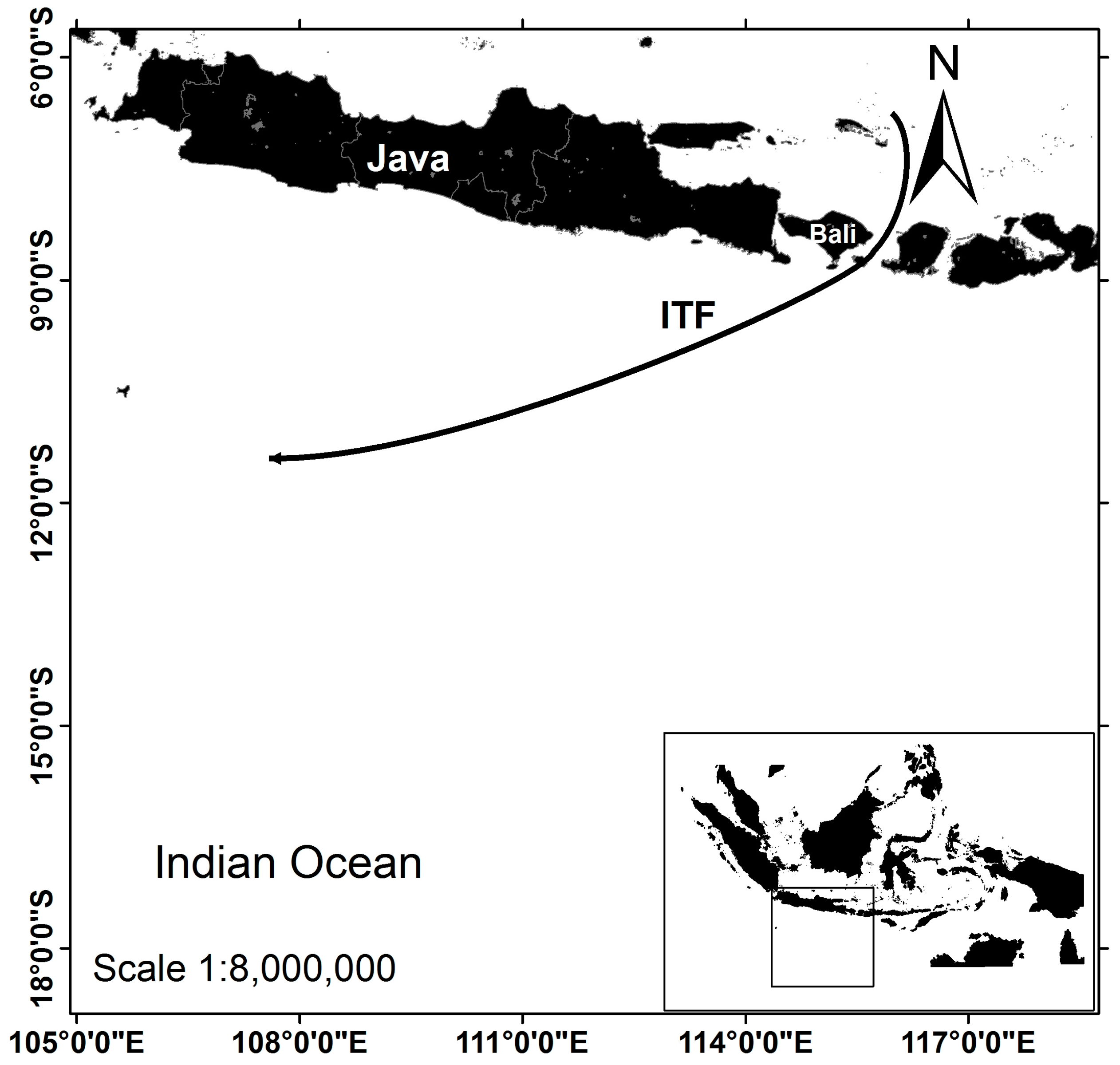
2.1. Study Area
2.2. Fisheries Data and Remotely Sensed Environmental Data
2.3. Scatterplot Smoothers
2.4. Fisheries Data Classification
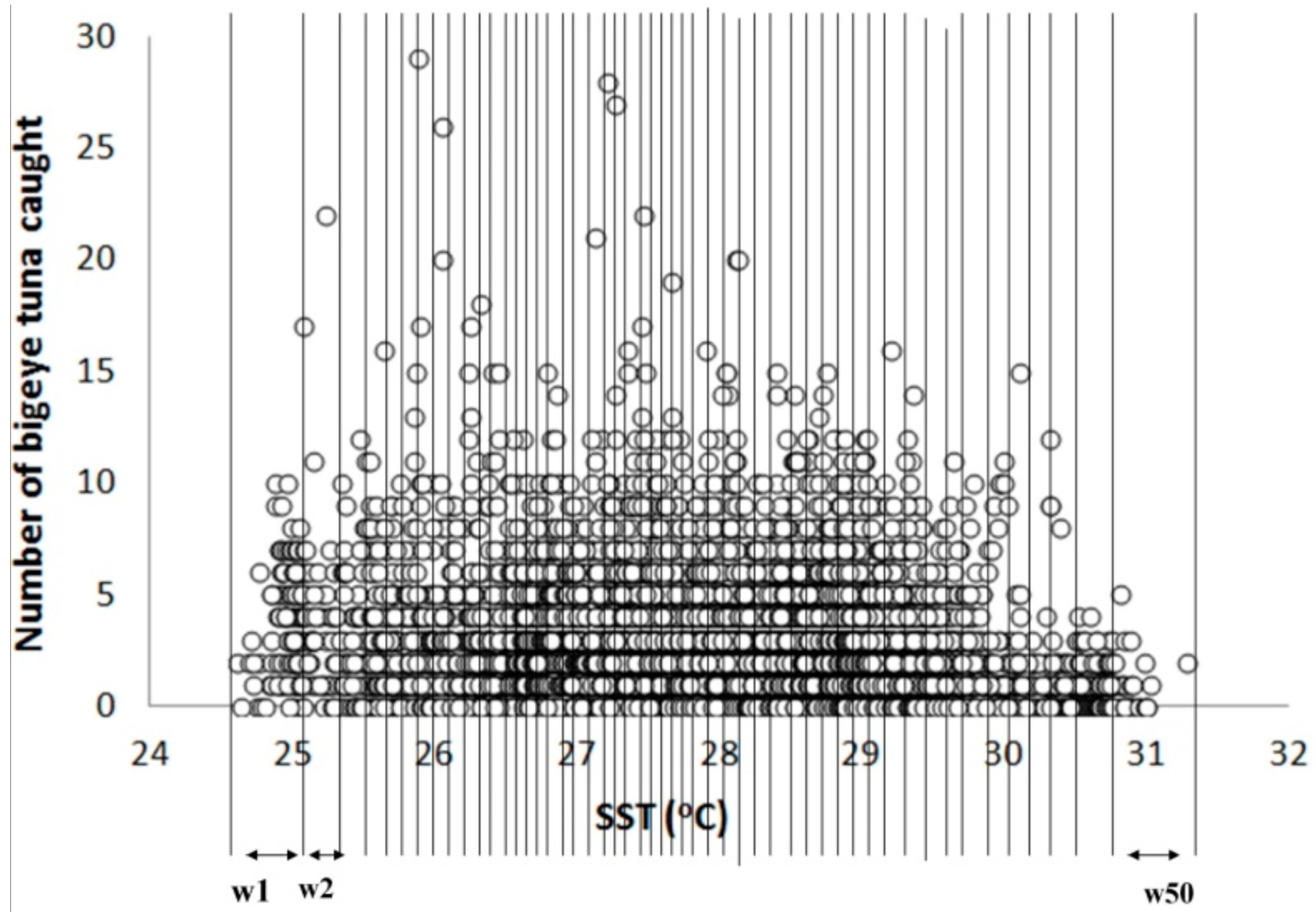
2.5. Generating the Optimum Range of Environmental Variables
2.6. Generating a Simple Predicted Distribution Map
3. Results and Discussion
3.1. Scatter Smoothers
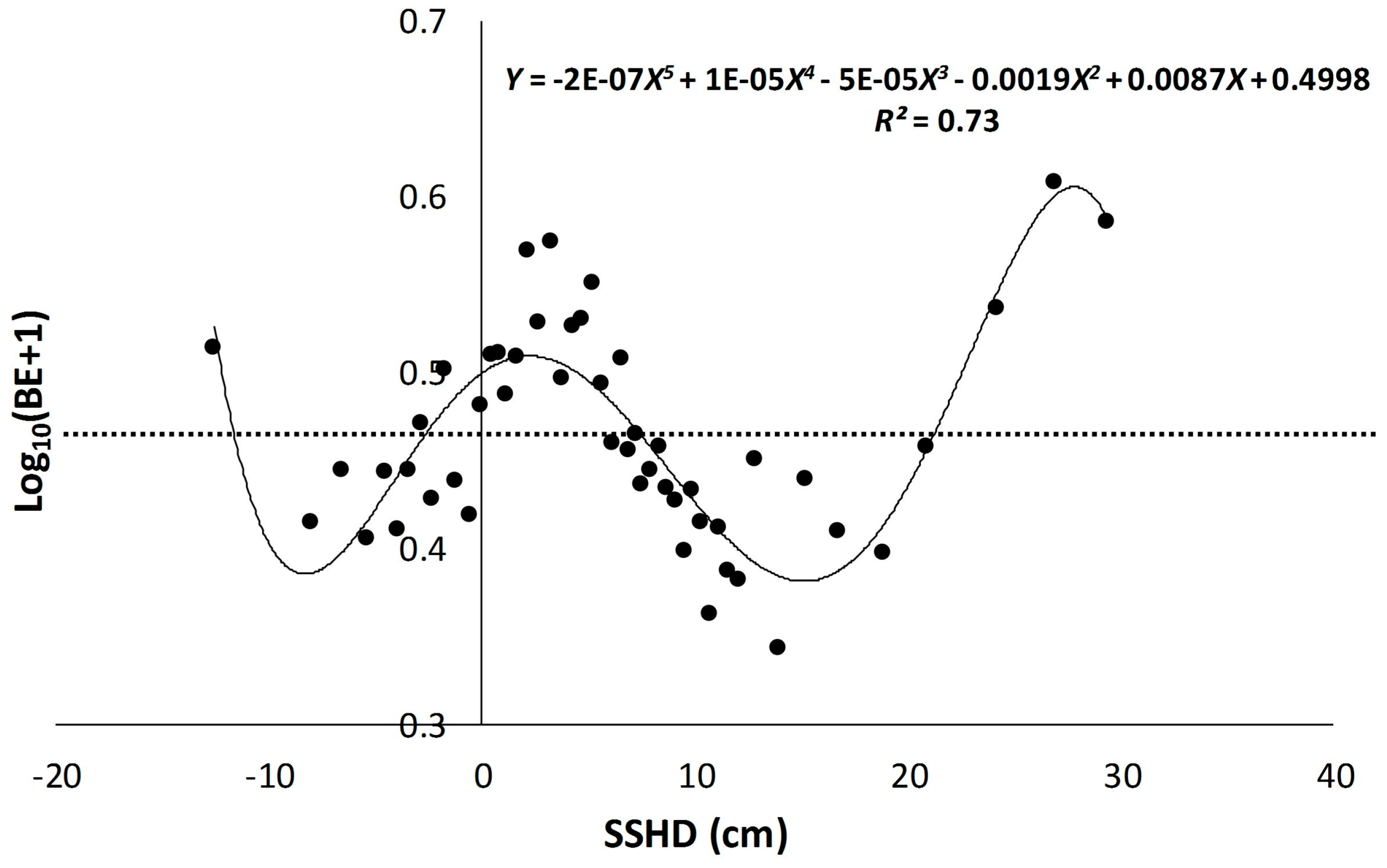
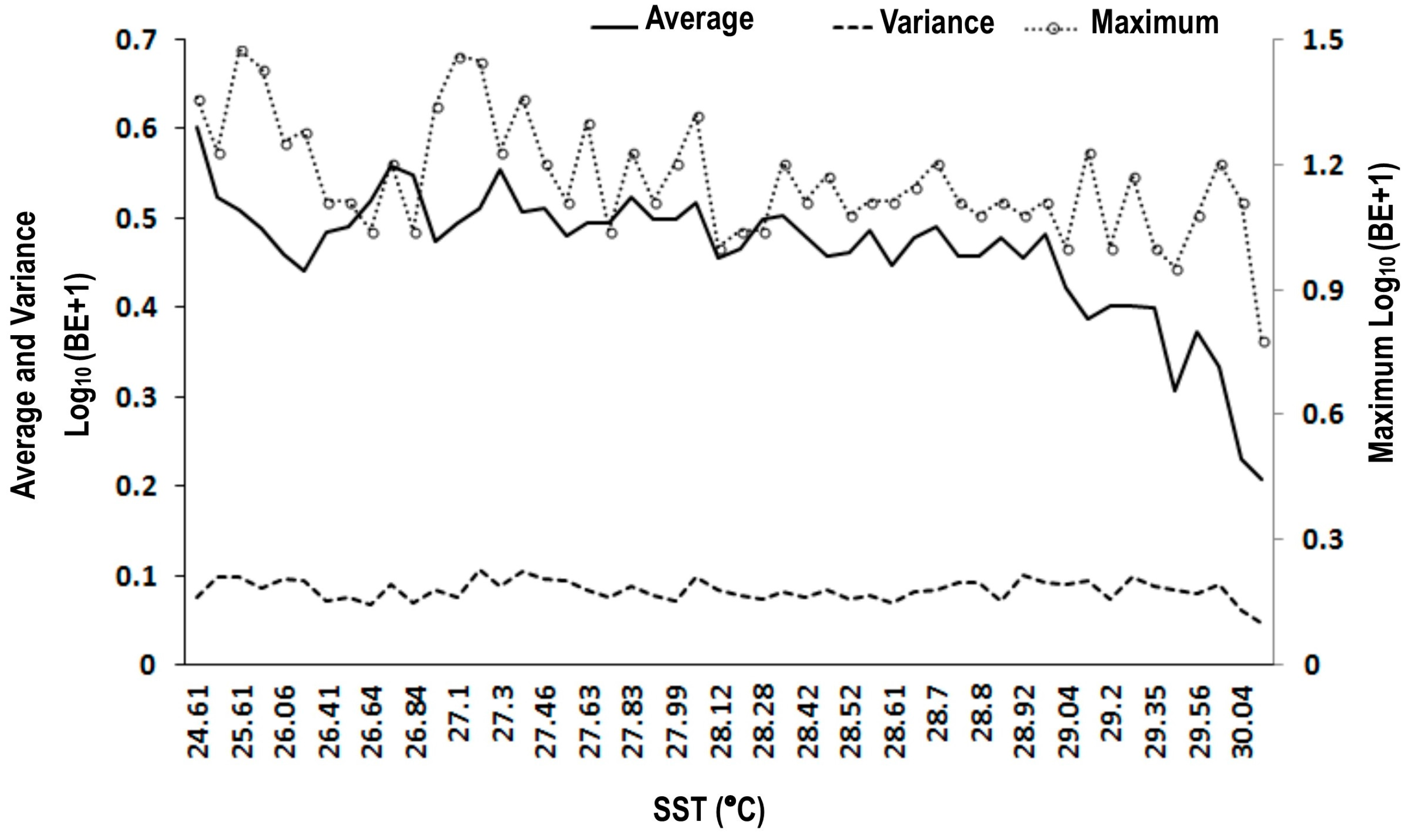
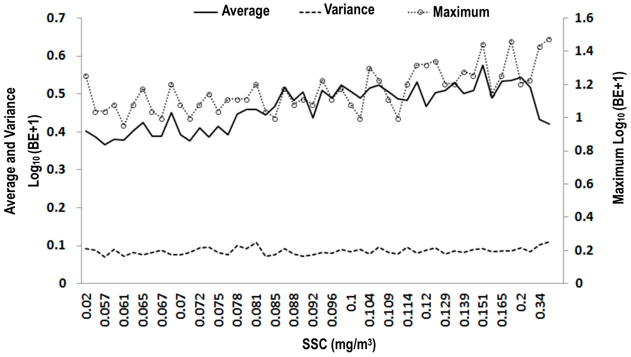
3.2. Relationship between Environmental Factors and Bigeye Tuna Caught
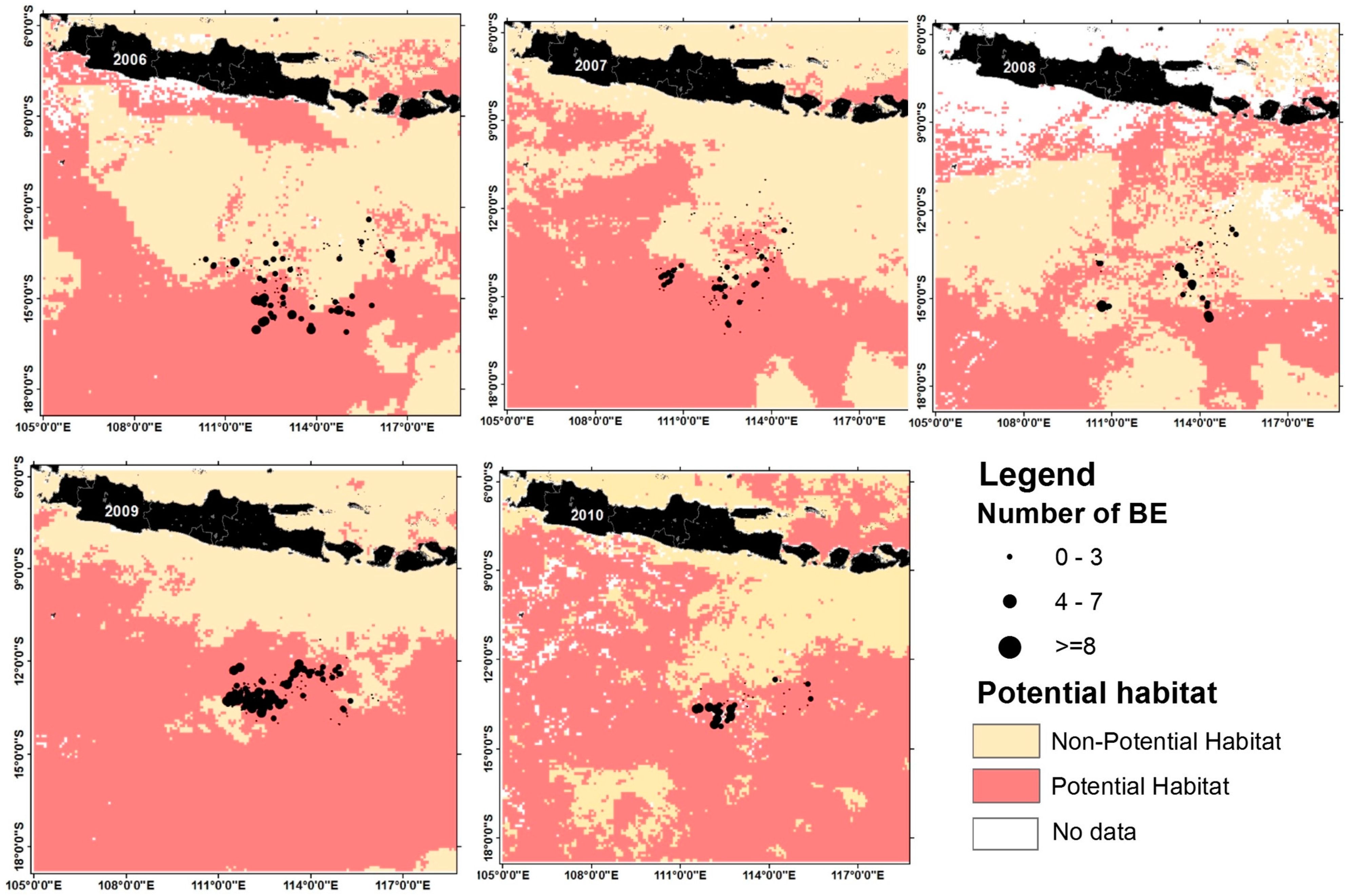
3.3. Model Validation and Potential Habitat Prediction
3.4. Relationship between Ocean Dynamics and Preferred Habitat for Bigeye Tuna
4. Conclusions
Acknowledgments
Author Contributions
Conflicts of Interest
References
- Pillai, N.G.K.; Satheeshkumar, P. Biology, fishery, conservation and management of Indian Ocean tuna fisheries. Ocean Sci. J. 2012, 47, 411–433. [Google Scholar] [CrossRef]
- ISSF. ISSF Stock Status Ratings-2012—Status of the World Fisheries for Tuna. Available online: https://troubledwatersfilm.files.wordpress.com/2015/01/issf-2012-status-of-the-world-fisheries-for-tuna.pdf (accessed on 5 December 2015).
- Wujdi, A.; Rochman, F.; Jatmiko, I. Length Distribution and Sex Ratio to Investigate Spawn Eligibility of Bigeye Tuna (Thunnus obesus Lowe, 1839) in the Indian Ocean (in Indonesian). Widyariset 2016, 2, 67–76. [Google Scholar] [CrossRef]
- Howell, E.A.; Hawn, D.R.; Polovina, J.J. Spatiotemporal variability in Bigeye tuna (Thunnus obesus) dive behaviour in the Central North Pacific Ocean. Prog. Oceanogr. 2010, 86, 81–93. [Google Scholar] [CrossRef]
- Sund, P.N.; Blackburn, M.; William, F. Tunas and their environment in the Pacific Ocean: A review. Oceanogr. Mar. Biol. Ann. Rev. 1981, 19, 443–512. [Google Scholar]
- Brill, R.W.; Bigelow, K.A.; Musyl, M.K.; Fritsches, K.A.; Warrant, E.J. Bigeye tuna (Thunnus obesus) behavior and physiology and their relevance to stock assessments and fishery biology. Col. Vol. Sci. Pap. ICCAT 2005, 57, 142–161. [Google Scholar]
- Mohri, M.; Nishida, T. Distribution of bigeye tuna (Thunnus obesus) and its relationship to the environmental conditions in Indian Ocean based on the Japanese longline fisheries information. IOTC Proc. 1999, 2, 221–230. [Google Scholar]
- Pranowo, W.S.; Tisiana, A.; Nugraha, B.; Novianto, D.; Muawanah, U. Ocean-Climate Interaction of Eastern Indian Ocean for Tuna. Available online: http://wwa.iotc.org/sites/default/files/documents/2014/11/IOTC-2014-WPTT16-23_-_Ocean_climate_interaction.pdf (accessed on 5 December 2015).
- Pranowo, W. Fenomena di Laut Selatan Jawa Tersebut Kami Beri Nama “RATU”. Indones. Marit. Mag. 2014, 44, 44–45. [Google Scholar]
- Susanto, R.D.; MooreII, T.S.; Marra, J. Ocean color variability in the Indonesian Seas during the SeaWiFS era. Geochem. J. 2006, 7. [Google Scholar] [CrossRef]
- Sachoemar, S.; Yanagi, T. Temporal and Spatial Variability of Sea Surface Temperature within Indonesian Regions Revealed by Satellite Data. Rep. Res. Inst. Appl. Mech. Kyushu Univ. 2013, 145, 37–41. [Google Scholar]
- Zainuddin, M.; Kiyofuji, H.; Saitoh, K.; Saitoh, S.-I. Using multi-sensor satellite remote sensing and catch data to detect ocean hot spots for albacore (Thunnus alalunga) in the northwestern North Pacific. Deep Sea Res. Part II Top. Stud. Oceanogr. 2006, 53, 419–431. [Google Scholar] [CrossRef]
- Sprintall, J.; Wijffels, S.E.; Molcard, R.; Jaya, I. Direct Estimates of the Indonesian Throughflow Entering the Indian Ocean: 2004–2006. J. Geophys. Res. 2009, 114. [Google Scholar] [CrossRef]
- Gordon, A.L. Oceanography of the Indonesian Seas and Their Throughflow. Oceanography 2005, 18, 14–27. [Google Scholar] [CrossRef]
- Nishikawa, Y.; Honma, M.; Ueyanagi, S.; Kikawa, S. Average Distribution of Larvae of Oceanic Species of Scombroid Fishes, 1956–1981; Far Seas Fisheries Research Laboratory: Simizu, Japan, 1985; p. 99. [Google Scholar]
- Nishida, T.; Mohri, M.; Itoh, K.; Nakagome, J. Study of Bathymetry Effects on the Nominal Hooking Rates of Yellowfin Tuna (Thunnus albacares) and Bigeye Tuna (Thunnus obesus) Exploited by the Japanese Tuna Longline Fisheries in the Indian Ocean. Available online: http://citeseerx.ist.psu.edu/viewdoc/similar?doi=10.1.1.467.4954&type=ab (accessed on 6 November 2016).
- Chassot, E.; Bonhommeau, S.; Reygondeau, G.; Nieto, K.; Polovina, J.J.; Huret, M.; Dulvy, N.K.; Demarcq, H. Satellite remote sensing for an ecosystem approach to fisheries management. ICES J. Mar. Sci. 2011, 68, 651–666. [Google Scholar] [CrossRef]
- Klemas, V. Fisheries applications of remote sensing: An overview. Fish. Res. 2013, 148, 124–136. [Google Scholar] [CrossRef]
- Polovina, J.J.; Howell, E.A. Ecosystem indicators derived from satellite remotely sensed oceanographic data for the North Pacific. ICES J. Mar. Sci. 2011, 62, 319–327. [Google Scholar] [CrossRef]
- Du, Y.; Qu, T.; Meyers, G.; Masumoto, Y.; Sasaki, H. Seasonal heat budget in the mixed layer of the southeastern tropical Indian Ocean in a high-resolution ocean general circulation model. J. Geophys. Res. 2005, 110. [Google Scholar] [CrossRef]
- Syamsuddin, M.L.; Saitoh, S.I.; Hirawake, T.; Bachri, S.; Harto, A.B. Effects of El Niño–Southern Oscillation events on catches of Bigeye Tuna (Thunnus obesus) in the eastern Indian Ocean of Java. Fish. Bull. 2013, 111, 175–188. [Google Scholar] [CrossRef]
- Kasma, E.; Osawa, T.; Adnyana, I.W.S. Estimation of primary productivity for tuna in Indian Ocean. Ecotrophic J. Environ. Sci. 2010, 4, 86–91. [Google Scholar]
- Maritorena, S.; D’Andon, O.H.F.; Mangin, A.; Siegel, D.A. Merged satellite ocean color data products using a bio-optical model: Characteristics, benefits and issues. Remote Sens. Environ. 2010, 114, 1791–1804. [Google Scholar] [CrossRef]
- Abbot, M.R.; Letelier, R.M. Chlorophyll Fluorescence (MODIS Product Number 20). Available online: http://citeseerx.ist.psu.edu/viewdoc/summary?doi=10.1.1.551.9575 (accessed on 3 June 2016).
- Setiawati, M.D.; Sambah, A.B.; Miura, F.; Tanaka, T.; Ass-syakur, A.R. Characterization of bigeye tuna habitat in the Southern Waters off Java-Bali using remote sensing data. Adv. Space Res. 2015, 55, 732–746. [Google Scholar] [CrossRef]
- Neill, W.H.; Chang, R.K.C.; Dizon, A.E. Magnitude and ecological implications of thermal inertia in skipjack tuna Katsuwonus pelamis (Linneaus). Environ. Biol. Fish. 1976, 1, 61–80. [Google Scholar] [CrossRef]
- Mugo, R.; Saitoh, S.I.; Nihara, A.; Kuroyama, T. Habitat characteristics of skipjack tuna (Katsuwonus pelamis) in the Western North Pasific. Fish. Oceanogr. 2010, 19, 382–396. [Google Scholar] [CrossRef]
- Bailey, C.; Dwiponggo, A.; Marahudin, F. Indonesia Marine Capture Fisheries (1987). Available online: http://pubs.iclarm.net/libinfo/Pdf/Pub%20SR76%2010.pdf (accessed on 3 June 2016).
- Osawa, T.; Julimantoro, S. Study of Fishery Ground around Indonesia Archipelago Using Remote Sensing Data. In Adaptation and Mitigation Strategies for Climate Change; Springer: Tokyo, Japan, 2010; pp. 57–69. [Google Scholar]
- Laurs, R.M.; Fiedler, P.C.; Montgomery, D.R. Albacore tuna catch distributions relative to environmental features observed from satellites. Deep Sea Res. Part A Oceanogr. Res. Pap. 1984, 31, 1085–1099. [Google Scholar] [CrossRef]
- Zainuddin, M.; Saitoh, K.; Saitoh, S.I. Albacore (Thunnus alalunga) fishing ground in relation to oceanographic condition in the Western North Pacific Ocean using remotely sensed satellite data. Fish. Oceanogr. 2008, 17, 61–73. [Google Scholar] [CrossRef] [Green Version]
- Hastie, T.J.; Tibshirani, R.J. Generalized Additive Models; CRC Press: New York, NY, USA, 1990. [Google Scholar]
- Muhling, B.A.; Reglero, P.; Ciannelli, L.; Alvarez-Berastegui, D.; Alemany, F.; Lamkin, J.T.; Roffer, M.A. Comparison between environmental characteristics of larval bluefin tuna Thunnus thynnus habitat in the Gulf of Mexico and Western Mediterranean Sea. Mar. Ecol. Prog. Ser. 2013, 486, 257–276. [Google Scholar] [CrossRef]
- Reygondeau, G.; Maury, O.; Beugrand, G.; Fromentin, J.M.; Fonteneau, A.; Curry, P. Biogeography of tuna and billfish communities. J. Biogeogr. 2012, 39, 114–129. [Google Scholar] [CrossRef]
- Feng, M.; McPhaden, M.J.; Xie, S.P.; Hafner, J. La Niña forces unprecedented Leeuwin Current warming in 2011. Sci. Rep. 2013, 3. [Google Scholar] [CrossRef] [PubMed]
- Soman, M.K.; Slingo, J. Sensitivity of the Asian summer monsoon to aspects of sea surface temperature anomalies in the tropical Pacific Ocean. Q. J. R. Meteorol. Soc. 1997, 123, 309–336. [Google Scholar] [CrossRef]
- Wyrtki, K. Physical Oceanography of the Southeast Asia Waters. Available online: http://escholarship.org/uc/item/49n9x3t4#page-3 (accessed on 2 July 2016).
- Zagaglia, C.R.; Lorenzzetti, J.A.; Stech, J.L. Remote sensing data and longline catches of yellowfin tuna (Thunnus alalunga) in the Equatorial Atlantic. Remote Sens. Res. 2004, 93, 267–281. [Google Scholar] [CrossRef]
- Ocean Color. Available online: https://oceancolor.gsfc.nasa.gov/cgi/l3 (accessed on 5 June 2016).
- Environmental Data Connector. Available online: http://www.pfeg.noaa.gov/products/EDC/ (Accessed on 17 June 2013).
- Andrade, H.A.; Garcia, C.A.E. Skipjack tuna fishery in relation to sea surface temperature off the southern Brazilian coast. Fish. Oceanogr. 1999, 8, 245–254. [Google Scholar] [CrossRef]
- Wolf, T.; McGregor, G. The development of a heat wave vulnerability index for London, United Kingdom. Weather Clim. Extrem. 2013, 1, 59–68. [Google Scholar] [CrossRef] [Green Version]
- Pranowo, W.; Philips, H.; Wijffels, S. Upwelling Event 2003 Along South Java Sea and Lesser Sunda Islands. J. Segara 2005, 1, 63–67. [Google Scholar]
- Druon, J.N. Habitat mapping of the Atlantic bluefin tuna derived from satellite data: Its potential as a tool for the sustainable management of pelagic fisheries. Mar. Policy 2010, 34, 293–297. [Google Scholar] [CrossRef]
- Syamsuddin, M.; Saitoh, S.-I.; Hirawake, T.; Syamsuddin, F.; Zainuddin, M. Interannual variation of bigeye tuna (Thunnus obesus) hotspots in the eastern Indian Ocean off Java. Int. J. Remote Sens. 2016, 37, 2087–2100. [Google Scholar] [CrossRef]


| Year | Month | Date | Latitude | Longitude | BE | SST | SSC | SSHD |
|---|---|---|---|---|---|---|---|---|
| 2006 | 2 | 8 | −14.4167 | 111.6667 | 2 | 28.12 | 0.06 | −7.84 |
| 2006 | 2 | 8 | −13.1667 | 113.0333 | 2 | 28.44 | 0.08 | −2.35 |
| 2006 | 2 | 8 | −14.15 | 112.75 | 3 | 28.52 | 0.08 | −6.52 |
| 2006 | 2 | 8 | −13.3333 | 114.6667 | 5 | 28.61 | 0.09 | −6.72 |
| 2010 | Mi | Di | Lati | Loni | BEi | SSTi | SSCi | SSHDi |
| Environmental Variables | x | λ | Weight |
|---|---|---|---|
| SST | 0.45 | 1.87 | 0.62 |
| SSC | 0.48 | 1.87 | 0.65 |
| SSHD | 0.33 | 1.87 | 0.45 |
| Model | p-Value | R2 |
|---|---|---|
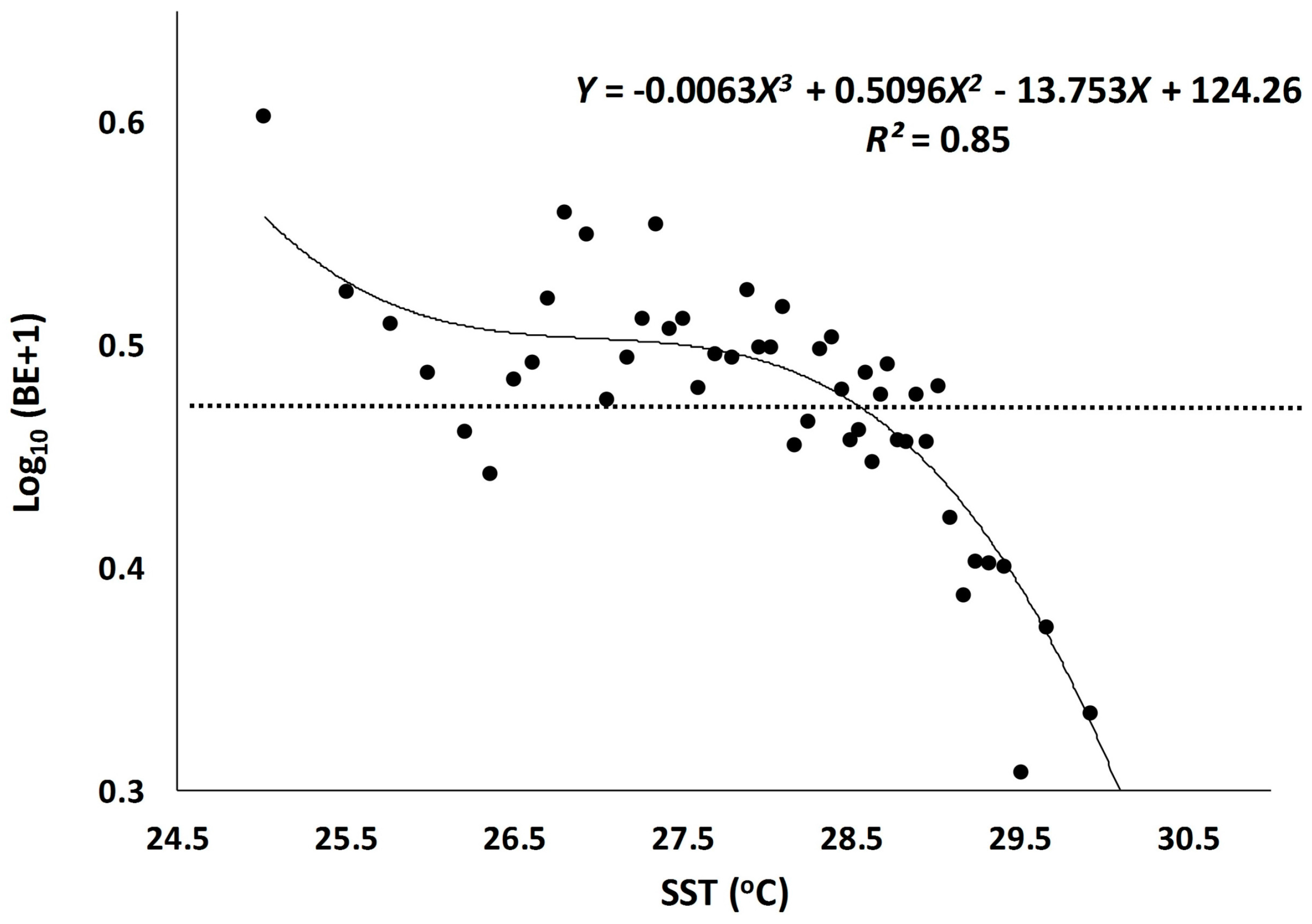
| SST | 3.7 × 10⁻¹⁹ | 0.85 |
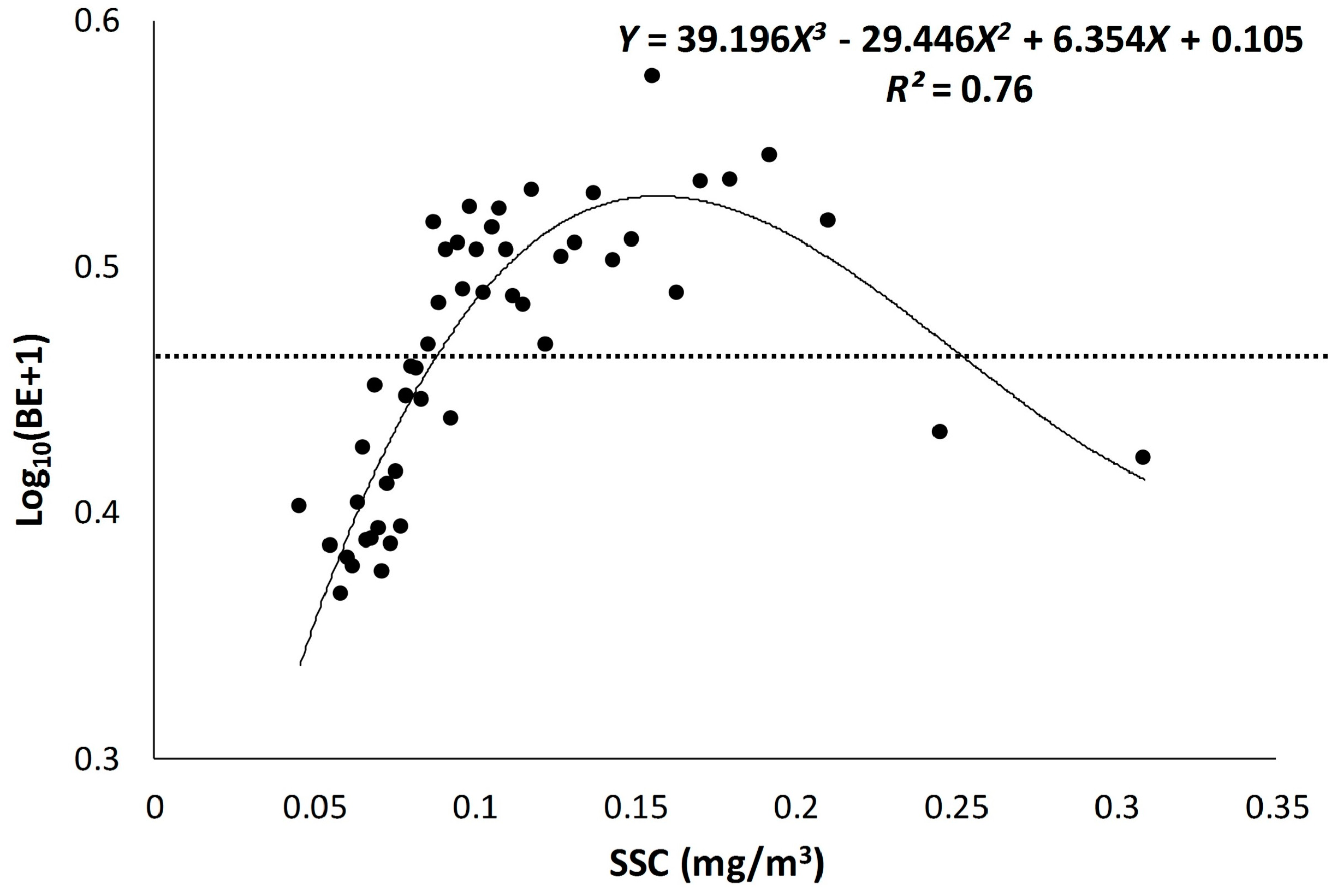
| SSC | 3.12 × 10⁻¹⁴ | 0.78 |
| SSHD | 1.53 × 10⁻¹¹ | 0.73 |
| Fisheries In-Situ Data | Potential Habitat | ||
|---|---|---|---|
| Yes | No | ||
| Tuna catches | Yes | 210 (A) | 51 (C) |
| No | 262 (B) | 128 (D) | |
© 2017 by the authors; licensee MDPI, Basel, Switzerland. This article is an open access article distributed under the terms and conditions of the Creative Commons Attribution (CC BY) license (http://creativecommons.org/licenses/by/4.0/).
Share and Cite
Setiawati, M.D.; Tanaka, T. Utilization of Scatterplot Smoothers to Understand the Environmental Preference of Bigeye Tuna in the Southern Waters off Java-Bali: Satellite Remote Sensing Approach. Fishes 2017, 2, 2. https://doi.org/10.3390/fishes2010002
Setiawati MD, Tanaka T. Utilization of Scatterplot Smoothers to Understand the Environmental Preference of Bigeye Tuna in the Southern Waters off Java-Bali: Satellite Remote Sensing Approach. Fishes. 2017; 2(1):2. https://doi.org/10.3390/fishes2010002
Chicago/Turabian StyleSetiawati, Martiwi Diah, and Tasuku Tanaka. 2017. "Utilization of Scatterplot Smoothers to Understand the Environmental Preference of Bigeye Tuna in the Southern Waters off Java-Bali: Satellite Remote Sensing Approach" Fishes 2, no. 1: 2. https://doi.org/10.3390/fishes2010002