GPU Accelerated Image Processing in CCD-Based Neutron Imaging


1
Chair of Biomedical Physics, Department of Physics and Munich School of BioEngineering, Technical University of Munich, 85748 Garching, Germany
2
Heinz Maier-Leibnitz Zentrum, Technical University of Munich, 85748 Garching, Germany
3
Department of Diagnostic and Interventional Radiology, Klinikum rechts der Isar, Technical University of Munich, 81675 München, Germany
*
Author to whom correspondence should be addressed.
J. Imaging 2018, 4(9), 104; https://doi.org/10.3390/jimaging4090104
Submission received: 17 July 2018
/
Revised: 9 August 2018
/
Accepted: 9 August 2018
/
Published: 21 August 2018
Abstract
:Image processing is an important step in every imaging path in the scientific community. Especially in neutron imaging, image processing is very important to correct for image artefacts that arise from low light and high noise statistics. Due to the low global availability of neutron sources suitable for imaging, the development of these algorithms is not in the main scope of research work and once established, algorithms are not revisited for a long time and therefore not optimized for high throughput. This work shows the possible speed gain that arises from the usage of heterogeneous computing platforms in image processing along the example of an established adaptive noise reduction algorithm.
1. Introduction
Non-destructive testing is a term comprising several important techniques to probe specimen for certain characteristics without the need to physically alter them and has a vast field of applications. One area inside these non-destructive testing methods is radiographic as well as tomographic imaging of samples with e.g., X-rays or neutrons. In those imaging techniques, a sample is placed inside an incident beam. The characteristics of the beam are changed by the introduction of the sample and this change can be recorded by suitable detectors such as scintillation counters or cameras to gain information about the sample. In neutron imaging, the intensity of the incident beam is decreased inside the sample by several different interactions such as absorption, coherent and incoherent nuclear scattering and magnetic dipole interaction. As the interaction cross-sections depend on the composition of the atomic nucleus, they vary wildly over the periodic table and can even have significant differences for different isotopes of the same element as can be seen in Table 1.
Therefore, the attenuation of a sample is dependent on its material composition and is pictured in a 2D image in projections or in a 3D array of voxels in a tomographic acquisition. Neutrons are mostly produced in research reactors by nuclear fission or in spallation sources and are characterised by their temperature which is linked to their energy via
Mostly thermal and cold neutrons with temperatures around 25 K to 300 K are used for imaging [2]. Compared to X-ray imaging, a typical neutron imaging setup has a lower total flux and the global availability of neutron beam-time is magnitudes lower [3,4]. As the cross-sections of neutron interactions are strongly energy dependent, in general the spectrum of the incident beam has to be well known in order to being able to quantify the results. Therefore, not all neutron sources are equally well suited for imaging applications. This is why it is essential to maximise usable beam-time and to get the most of the acquired images with suitable image processing. Furthermore, a fast image-processing work-flow allows scientist to perform dynamic measuring rows and to directly assure the quality of the acquired images on-site. Especially in medical imaging in the X-ray domain, GPU based image processing is well established and has shown potential for speed increase in several orders of magnitudes [5]. Noise reduction is an important first step of all image pipelines and therefore chosen as an example in this work. GPU-based video denoising has also been demonstrated with speed gains [6]. However, the application to neutron imaging has not been shown. Furthermore, the chosen implementation shows some optimisations that are transferable to a wide range of image-processing tasks not only in neutron imaging but in general to all pixel based imaging techniques.
2. Materials and Methods
2.1. Setup
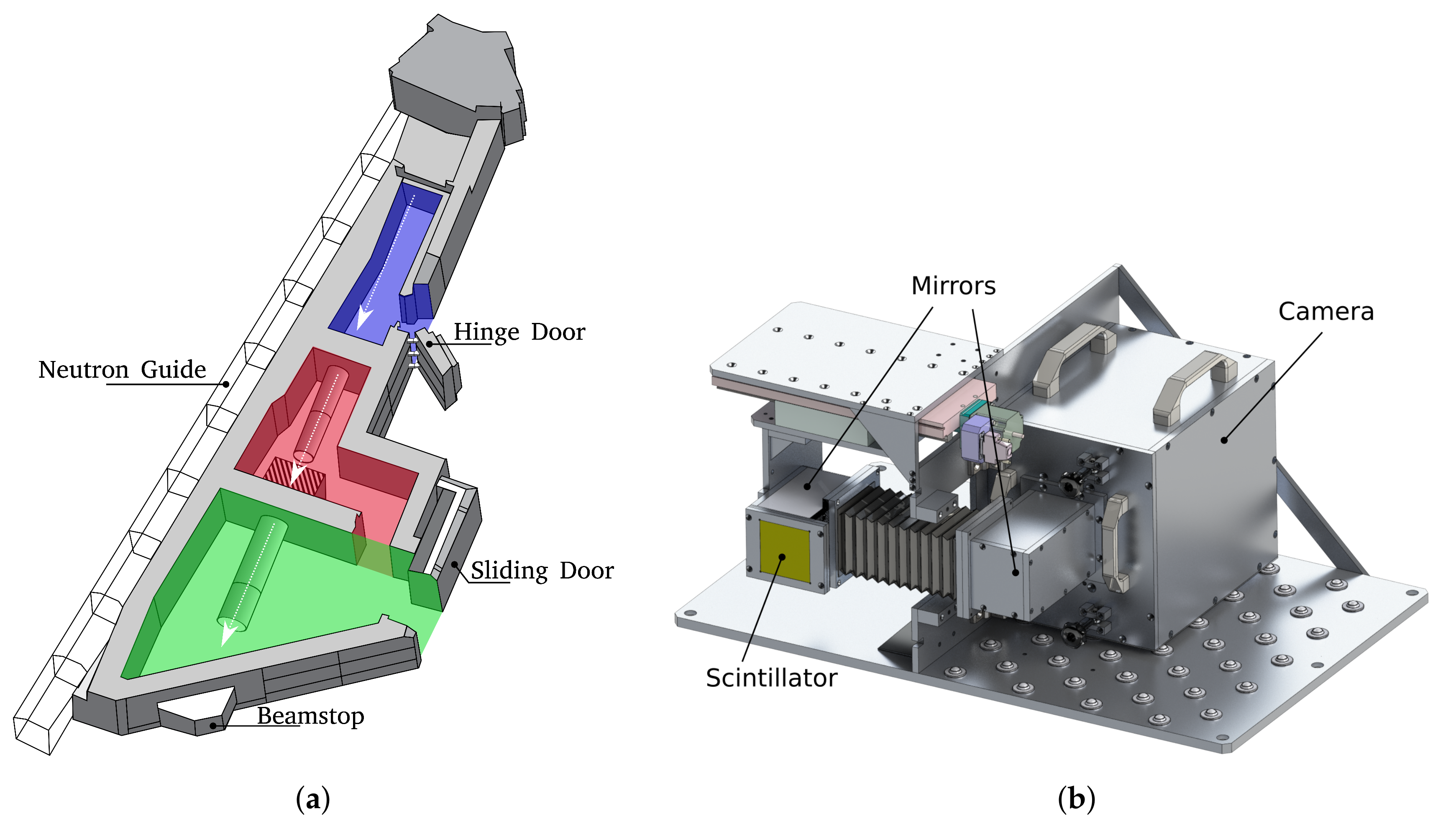
The measurements for this work were carried out at the Advanced Neutron Tomography and Radiography Experimental System (ANTARES) inside the research reactor neutron source facility Forschungs–Neutronenquelle Heinz–Maier–Leibnitz (FRM II). The cold neutron source used in the experiment has a temperature of about 25 K [7]. The shielding hutch of the ANTARES has three separated compartments, of which the first is used for beam- and spectrum shaping devices, amongst them being a mechanical velocity selector, a double crystal monochromator or interference gratings that can be used for grating based phase contrast imaging [8]. The detection system consists of a shielded detector box holding an Andor Ikon L CCD camera by Oxford Instruments, Abingdon, UK, with 2048 pixels in each dimension. A two-mirror beam-path allows the camera to be placed outside the direct neutron beam-path. A schematic drawing of the setup and the detector is shown in Figure 1. Measurements were done with an 18 mm pinhole, resulting in an L/D ratio of 500 at the sample position and an effective pixel size of about 27 μm.
2.2. Noise Removal
The images taken with the setup above suffer from noise stemming from various sources. Besides electronic and thermal noise as well as readout noise from the camera, the main noise source in neutron imaging experiments that deteriorate image quality are high energy -particles that are produced in nuclear reactions of neutrons inside material in and around the experimental setup. Those high energy particles lead to bright spots when they hit the detector, which are referred to in this work as gamma spots. An example of the resulting artefact of such gamma spots is shown in Figure 2.
Two bright spots with a bright surrounding can be seen in this image. These spots results from an excess charge production on the CCD sensor, that can no longer be contained in the potential well of one single pixel. Furthermore a streak in the readout direction of the camera can be seen emerging from the primary interaction position. This is due to the fact, that charge transfers from pixel to pixel in the readout direction are facilitated due to the inner workings of a CCD camera. This streak therefore is more prominent at higher readout frequencies and lower potential well depths of the pixels. The problem with these gamma spots is, that a global correction such as Gaussian blurring or taking the median of the affected area decreases the resolution of the image due to the averaging nature of these filters. Adaptive filters, such as described by [9] circumvent this problem by adapting the size of the filter kernel to the strength of noise in the image. Their algorithm will be shortly summarized in the following. A Laplacian of Gaussian (LoG) filter is a well-known edge finding algorithm and is a convolution with the LoG kernel, that can be written in the discrete form
with the abbreviation
where and are denoting the position of the kernel element in each dimension and is the standard deviation. The resulting edge-image shows high intensities at pixels, where there is a fast change in image intensity in the raw image. As higher noise levels lead to sharper edges, the edge-image can be thresholded in several levels, to adjust the size of a subsequent median kernel. In that way, the median filter only affects areas, in which noise above a certain threshold is present and can be tuned to account for a larger neighbourhood when the gamma spots affect a larger area. To account for very bright and big spots, the threshold image for the median with a kernel size of 7 can additionally be binary-dilated.
2.3. Sample
To allow for reproducible results, three dimensional test arrays with a discrete uniform random gray value distribution in the open interval were created with a size of 1024 pixels in each dimension to simulate an image stack. These images where used to profile both the running time of the benchmark implementation as well as our optimised parallel implementation. The demonstration of the noise-removal abilities of the presented implementation is shown on images of polymer electrolyte membrane fuel cells (PEMFCs) acquired at the ANTARES and explained in more detail in [10].
2.4. Implementation
A reference implementation of the described algorithm was done in Python 2.7 to allow for detailed profiling and identification of the most timely image processing steps needed which have been identified to be the convolution with the precomputed LoG kernel and the median filtering. In general, a convolution in the image domain can be expressed as a multiplication in the Fourier domain and the needed algorithms to do a Fast Fourier Transform (FFT) are well known and constantly improved [11,12,13]. However, for small kernels convolution is faster and has less memory overhead than FFT [14]. Furthermore, there is no convolution kernel that defines the median, as the median is based on order statistics. Therefore a pixel-wise implementation is chosen both for the reference and the optimized version. The optimised implementation is done in OpenCL with the Python API PyOpenCL [15]. OpenCL was chosen because of it being an open royalty-free standard that is portable across a lot of different computing architectures such as CPUs and GPUs as well as other programmable hardware such as FPGAs and DSPs [16]. OpenCL implements an image object, which has a dedicated underlying memory model that allows the use of samplers for reading. As these samplers allow for automatic bounds-checking, the algorithm gets a lot simpler as manual bounds-checking has to be done no longer. Further more, the image model allows caching of pixel values, so that subsequent access to pixels in the neighbourhood of a lately read-out pixel are accelerated. Memory transfer from host to device is done with PyOpenCL and each transfer as well as each kernel enqueueing is enriched with an OpenCL event that allows to extract exact timing information for memory transfers as well as kernel executions on the device. The source code of the OpenCL kernels is shown in Appendix A.
3. Results and Discussion
3.1. Profiling
The profiling of the implementation in python shows that the running time of the convolution and the median scales linearly with the pixel count of the input array as can be seen in Figure 3. Furthermore, the median additionally scales with the footprint or region size.
From this measurements, the time needed for an pixel image can be extrapolated. To get an estimate, for the running time in a real application, the running time of the median kernels has to be multiplied with the noise density in each threshold bin, as the median only has to be executed on these values, which reduces running time. This is not the case for the convolution. Li et al. mention noise densities of 13.35%, 1.68% and 0.33% for the corresponding median sizes of 3, 5 and 7 [9]. With these noise densities, the running time of the complete algorithm is dominated by the time taken in the convolution step and is around 1 s for one image compared to 5 s mentioned in the same source.
3.2. Optimisation
In the OpenCL implementation, the input data, namely the array holding the LoG coefficients and the raw input images, has to be transferred from host to device. Subsequently the convolution, thresholding, dilation and the adaptive median is run on the device. The timing of these steps on the same random images used before is done on one Tesla K10 G2 by Nvidia, Santa Clara, CA, USA, and shown in Figure 4.
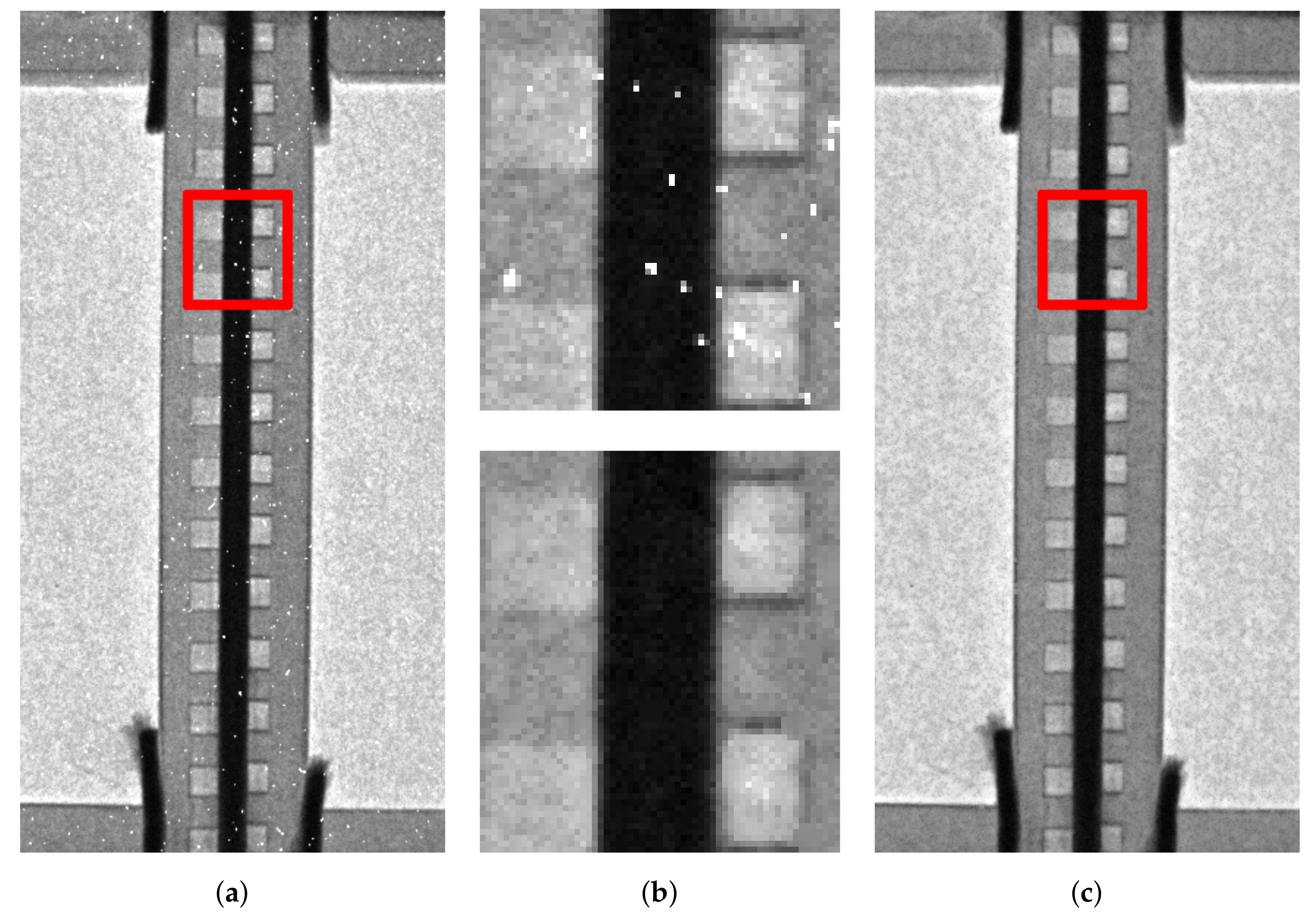
This timing suggests a possible speed increase of 160 times compared to the original implementation. Transfer time back to the host is not included in the calculation as it strongly depends on the speed of the desired output storage but in general should be in the order of the time needed for the input. The time needed in this implementation is not dependent on the noise density or the threshold levels as the kernel is run on every input pixel in parallel as long as the input can be mapped to the available number of work items on the GPU device. If the size of input data is increased, the running time increases discretely with each new memory block. As an example, an image stack with a z-size between 65 and 128 would take double the time as the shown timing. The running time can further be decreased by interleaving the memory operations with the calculation. On modern graphics hardware, the input copy of a subsequent stack can happen while the calculations are done for the previous input. Conversely, the output of the previous result can be done during the calculation of the subsequent array. If implemented that way, the running time for a stack of 640 images is calculated to be around 4 s. As this implementation is highly parallelised, if higher speed is needed the algorithm can be run on several OpenCL devices at parallel. The application of the filter to an in-situ radiography of a fuel-cell is shown in Figure 5.
This work shows, that efficient parallel programming on GPUs is a suitable technique in image processing for CCD-based neutron imaging as a large range of image processing algorithms can be implemented in that way. If the processing-chain gets longer, the overhead of memory operations from host-device transfers can be more and more neglected against the speed gained from parallel execution. We showed, that even pixel-based algorithms and algorithms which have no formulation as a convolution kernel can be efficiently implemented on GPU to allow beam-line users a real-time feedback regarding image quality. Further work in this direction could be done in the GPU implementation of the complete imaging toolchain from background subtraction and flat-field correction up to implementation of dynamic image statistics such as pixel-wise standard deviations to allow e.g., for real-time corrections of intensity fluctuations of neutron sources.
Author Contributions
Software, Data Curation, Visualization and Writing — Original Draft Preparation J.S.; Resources M.S.; Project Administration, Funding Acquisition, review and editing M.S. and F.P.; Supervision F.P.
Funding
We acknowledge financial support through the DFG (Gottfried Wilhelm Leibniz program) and the BMBF (project 05K16WO8, NeuRoFast).
Acknowledgments
The authors would like to thank Simon Thiele, Riko Moroni and Matthias Breitwieser from IMTEK, Freiburg for the collaboration with the fuel-cell measurements.
Conflicts of Interest
The authors declare no conflict of interest. The founding sponsors had no role in the design of the study; in the collection, analyses, or interpretation of data; in the writing of the manuscript, and in the decision to publish the results.
Abbreviations
The following abbreviations are used in this manuscript:
| API | Application Programming Interface |
| CPU | Central Processing Unit |
| DSP | Digital Signal Processor |
| FFT | Fast Fourier Transform |
| FPGA | Field Programmable Gate Array |
| GPU | Graphics Processing Unit |
| LoG | Laplacian of Gaussian |
Appendix A. Source Code
This section lists the OpenCL kernels developed in this work and used for benchmarking.
Appendix A.1. LoG Convolution
		   1 __kernel void LoG(__read_only image3d_t d_image,
		   2 __read_only image3d_t d_coefficients,
		   3 __write_only image3d_t d_out_image,
		   4 int size, // The dimension of the convolution kernel
		   5 int offset_x, // optional if origin is not at (0,0)
		   6 int offset_y)
		   7 {
		   8 // Get the work element:
		   9 int x_i = get_global_id(0)+offset_x;
		   10 int y_i = get_global_id(1)+offset_y;
		   11 int z   = get_global_id(2);
		   12 //Initialise values:
		   13 float gauss_laplacian = 0.0;
		   14 float weight = 0.0;
		   15 int get_x = 0;
		   16 int get_y = 0;
		   17 int offset = (size-1)/2;
		   18 // Convolution:
		   19 for ( int y = y_i-offset; y <= y_i+offset; y++)
		   20 {
		   21 get_x = 0;
		   22 for ( int x = x_i-offset; x <= x_i+offset; x++)
		   23 {
		   24 weight = read_imagef(
		   25 d_coefficients,
		   26 sampler,
		   27 (int4)(get_x, get_y, 0, 0)). s0;
		   28 gauss_laplacian += (read_imagef(
		   29 d_image,
		   30 sampler,
		   31 (int4)(x, y, z, 0)). s0 * weight);
		   32 get_x++;
		   33 }
		   34 get_y++;
		   35 }
		   36
		   37 // Write the output value to the result array:
		   38 write_imagef(
		   39 d_out_image,
		   40 (int4)(x_i, y_i, z, 0),
		   41 (float4)(gauss_laplacian));
		   42 }
Listing 1.
OpenCL kernel used for convolution of an input image with a coefficient image.
Appendix A.2. Adaptive Median
                        1 __kernel void a_median(__read_only image3d_t d_image,
			2 __read_only image3d_t d_mask,
			3 __write_only image3d_t d_out_image,
			4 int t_low,
			5 int t_middle,
			6 int t_high, // Threshold levels
			7 int offset_x,
			8 int offset_y)
			9 {
			10 __private int x = get_global_id(0)+offset_x;
			11 __private int y = get_global_id(1)+offset_y;
			12 __private int z = get_global_id(2);
			13 __private int get_x, get_y, i, j;
			14 __private int pos = 0;
			15 __private float mask_value = read_imagef(
			16 d_mask,
			17 sampler,
			18 (int4)(x, y, z, 0)). s0;
			19 __private int size;
			20 // Set the median size:
			21 if (mask_value < t_low)
			22 {
			23 size = 1;
			24 }
			25 else if (t_low<=mask_value && mask_value<t_middle)
			26 {
			27 size = 3;
			28 }
			29 else if (t_middle<=mask_value && mask_value<t_high)
			30 {
			31 size = 5;
			32 }
			33 else if (mask_value>=t_high)
			34 {
			35 size = 7;
			36 }
			37 __private int offset = (size − 1)/2;
			38 __private int window_size = size*size;
			39 __private float window[81] = {0};
			40 __private float temp, median;
			41 __private float win_value;
			42 // Getting all values from the window
			43 for (get_x=-1*offset; get_x<=offset; get_x++)
			44 {
			45 for (get_y=-1*offset; get_y<=offset; get_y++)
			46 {
			47 win_value = read_imagef(
			48 d_image,
			49 sampler,
			50 (int4)(x+get_x, y+get_y, z, 0)). s0;
			51 window[pos] = win_value;
			52 pos++;
			53 }
			54 }
			55
			56 // Sorting the array in ascending order
			57 for (i = 0; i < window_size-1; i++) {
			58 for (j = 0; j < window_size-i-1; j++) {
			59 if (window[j] > window[j + 1]) {
			60 // swap elements
			61 temp = window[j];
			62 window[j] = window[j + 1];
			63 window[j + 1] = temp;
			64 }
			65 }
			66 }
			67 // Calculate and output median
			68 median = window[((size*size) − 1)/2];
			69 write_imagef(
			70 d_out_image,
			71 (int4)(x, y, z, 0),
			72 (float4)(median));
			73
			74 }
Listing 2.
OpenCL kernel used for an adaptive median with 3 different levels and three corresponding thresholds. The thresholded image is given as input in the mask.
References
- Sears, V. Neutron scattering lengths and cross sections. Neutron News 1992, 3, 26–37. [Google Scholar] [CrossRef]
- Schreyer, A. Physical Properties of Photons and Neutrons. In Neutrons and Synchrotron Radiation in Engineering Materials Science; Wiley-VCH Verlag GmbH & Co. KGaA: Hoboken, NJ, USA, 2008; pp. 79–89. [Google Scholar]
- Lehmann, E.H.; Ridikas, D. Status of Neutron Imaging—Activities in a Worldwide Context. Phys. Procedia 2015, 69, 10–17. [Google Scholar] [CrossRef]
- Anderson, I.S.; Andreani, C.; Carpenter, J.M.; Festa, G.; Gorini, G.; Loong, C.K.; Senesi, R. Research opportunities with compact accelerator-driven neutron sources. Phys. Rep. 2016, 654, 1–58. [Google Scholar] [CrossRef] [Green Version]
- Gulo, C.A.S.J.; Sementille, A.C.; Tavares, J.M.R.S. Techniques of medical image processing and analysis accelerated by high-performance computing: A systematic literature review. J. Real-Time Image Process. 2017, 1–18. [Google Scholar] [CrossRef]
- Pfleger, S.G.; Plentz, P.D.M.; Rocha, R.C.O.; Pereira, A.D.; Castro, M. Real-time video denoising on multicores and GPUs with Kalman-based and Bilateral filters fusion. J. Real-Time Image Process. 2017, 1–14. [Google Scholar] [CrossRef]
- Calzada, E.; Gruenauer, F.; Mühlbauer, M.; Schillinger, B.; Schulz, M. New design for the ANTARES-II facility for neutron imaging at FRM II. Nuclear Instrum. Methods Phys. Res. Sec. A Accel. Spectrom. Detect. Assoc. Equip. 2009, 605, 50–53. [Google Scholar] [CrossRef]
- Schulz, M.; Schillinger, B. ANTARES: Cold neutron radiography and tomography facility. J. Large-Scale Res. Facil. 2015, 1, A17. [Google Scholar] [CrossRef]
- Li, H.; Schillinger, B.; Calzada, E.; Yinong, L.; Muehlbauer, M. An adaptive algorithm for gamma spots removal in CCD-based neutron radiography and tomography. Nuclear Instrum. Methods Phys. Res. 2006, 564, 405–413. [Google Scholar] [CrossRef]
- Breitwieser, M.; Moroni, R.; Schock, J.; Schulz, M.; Schillinger, B.; Pfeiffer, F.; Zengerle, R.; Thiele, S. Water management in novel direct membrane deposition fuel cells under low humidification. Int. J. Hydrog. Energy 2016, 41. [Google Scholar] [CrossRef]
- Cooley, J.W.; Tukey, J.W. An algorithm for the machine calculation of complex Fourier series. Math. Comput. 1965, 19, 297–301. [Google Scholar] [CrossRef]
- Hegland, M. A self-sorting in-place fast Fourier transform algorithm suitable for vector and parallel processing. Numer. Math. 1994, 547, 507–547. [Google Scholar] [CrossRef]
- Moreland, K.; Angel, E. The FFT on a GPU. In Proceedings of the ACM SIGGRAPH/EUROGRAPHICS Conference On Graphics Hardware, San Diego, CA, USA, 26–27 July 2003; pp. 112–120. [Google Scholar]
- Fialka, O.; Čadík, M. FFT and convolution performance in image filtering on GPU. In Proceedings of the International Conference on Information Visualisation, London, UK, 5–7 July 2006; pp. 609–614. [Google Scholar] [CrossRef]
- Klöckner, A.; Pinto, N.; Lee, Y.; Catanzaro, B.; Ivanov, P.; Fasih, A. PyCUDA and PyOpenCL: A scripting-based approach to GPU run-time code generation. Parallel Comput. 2012, 38, 157–174. [Google Scholar] [CrossRef] [Green Version]
- Khronos Group. OpenCL Specification; Technical Report; Khronos Group: Beaverton, OR, USA, 2015. [Google Scholar]
- Jones, E.; Oliphant, T.; Peterson, P. SciPy: Open Source Scientific Tools for Python, 2001. Available online: http://www.scipy.org/ (accessed on 14 August 2018).
Figure 1.
A schematic sketch of the experimental hutch of the ANTARES setup is shown in (a) with the source-detector distance being approximately 9 m. In (b), the approximately 50 cm wide camera setup with a two-mirror beam-path and the scintillator is shown.
Figure 1.
A schematic sketch of the experimental hutch of the ANTARES setup is shown in (a) with the source-detector distance being approximately 9 m. In (b), the approximately 50 cm wide camera setup with a two-mirror beam-path and the scintillator is shown.

Figure 2.
Direct hits of two high energy particles on the detector of an Andor Ultra EMCCD camera by Oxford Instruments, Abingdon, UK, with a pixelsize of 16 μm. The camera is rotated 90° counter-clockwise; the readout direction of the camera is on the right side of the image.
Figure 2.
Direct hits of two high energy particles on the detector of an Andor Ultra EMCCD camera by Oxford Instruments, Abingdon, UK, with a pixelsize of 16 μm. The camera is rotated 90° counter-clockwise; the readout direction of the camera is on the right side of the image.
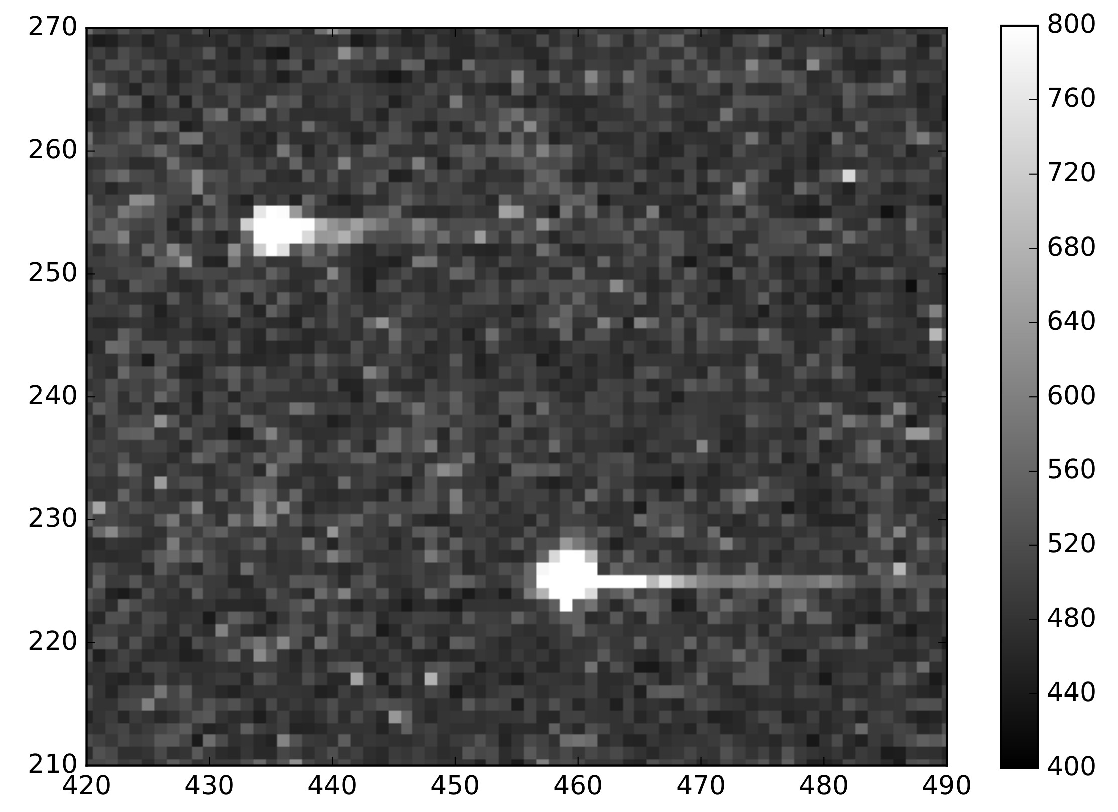
Figure 3.
Running time of the convolution and the median compared with the z-size of the three-dimensional array on which they are acting. All implementations are single-threaded and scale approximately linear. The median runs are two-dimensional median filters with the size being the x and y dimensions of the lookup-window. The convolution is done with the LoG Kernel with a size of and . Profiling implementations are done with scipy.ndimage [17].
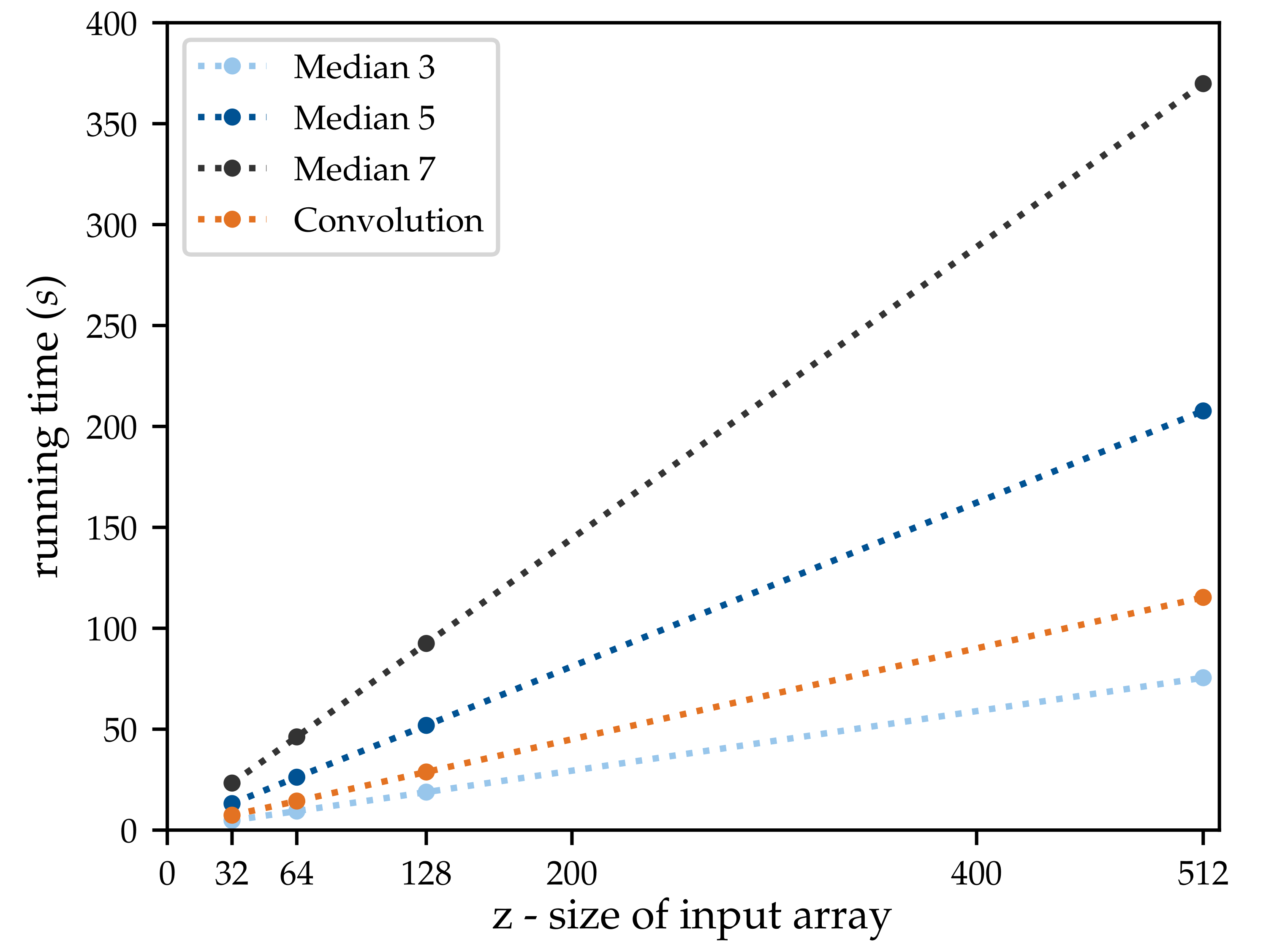
Figure 4.
Running time of an optimised version of the LoG adaptive median filter. Queue 1 lists all input timings, Queue 2 shows all numeric calculations. Each coloured block is one separate OpenCL kernel. Shown is the timing for one complete run of the algorithm on a 3D array with a size of random values between 0 and 1000 and thresholds at 50, 100 and 400 for median sizes of 3, 5 and 7.

Figure 5.
One projection of an in-situ neutron radiography of a fuel-cell. Subfigure (a) shows the uncorrected radiography, (c) shows the same radiography after correction. Red boxes indicate the regions shown in the magnification in (b) with the corrected version being below the uncorrected version. The fuel-cell is approximately 2.5 mm wide and the effective pixel size of the measurement was about 27 μm.


Table 1.
Interaction cross-sections of neutrons for some selected elements. All cross-sections are given in barn with 10 × 10−24 cm2. The scattering cross section and the absorption cross section are tabulated for 2200 m/s ( 25.30 meV) and taken from [1] and given without the error.
Table 1.
Interaction cross-sections of neutrons for some selected elements. All cross-sections are given in barn with 10 × 10−24 cm2. The scattering cross section and the absorption cross section are tabulated for 2200 m/s ( 25.30 meV) and taken from [1] and given without the error.
| Isotope | ||
|---|---|---|
| 1H | 82.02 | 0.3326 |
| H | 7.64 | 0.000519 |
| 5B | 5.24 | 767 |
| 13Al | 1.503 | 0.231 |
| 64Gd | 180 | 49,700 |
| Gd | 1044 | 259,000 |
© 2018 by the authors. Licensee MDPI, Basel, Switzerland. This article is an open access article distributed under the terms and conditions of the Creative Commons Attribution (CC BY) license (http://creativecommons.org/licenses/by/4.0/).
Share and Cite
MDPI and ACS Style
Schock, J.; Michael, S.; Pfeiffer, F. GPU Accelerated Image Processing in CCD-Based Neutron Imaging. J. Imaging 2018, 4, 104. https://doi.org/10.3390/jimaging4090104
AMA Style
Schock J, Michael S, Pfeiffer F. GPU Accelerated Image Processing in CCD-Based Neutron Imaging. Journal of Imaging. 2018; 4(9):104. https://doi.org/10.3390/jimaging4090104
Chicago/Turabian StyleSchock, Jonathan, Schulz Michael, and Franz Pfeiffer. 2018. "GPU Accelerated Image Processing in CCD-Based Neutron Imaging" Journal of Imaging 4, no. 9: 104. https://doi.org/10.3390/jimaging4090104
Note that from the first issue of 2016, this journal uses article numbers instead of page numbers. See further details here.