Python Non-Uniform Fast Fourier Transform (PyNUFFT): An Accelerated Non-Cartesian MRI Package on a Heterogeneous Platform (CPU/GPU)


1
Department of Radiology, University of Cambridge, Cambridge CB2 0QQ, UK
2
Graduate Institute of Biomedical Electronics and Bioinformatics, National Taiwan University, Taipei 106, Taiwan
J. Imaging 2018, 4(3), 51; https://doi.org/10.3390/jimaging4030051
Submission received: 5 January 2018
/
Revised: 13 February 2018
/
Accepted: 26 February 2018
/
Published: 8 March 2018
Abstract
:A Python non-uniform fast Fourier transform (PyNUFFT) package has been developed to accelerate multidimensional non-Cartesian image reconstruction on heterogeneous platforms. Since scientific computing with Python encompasses a mature and integrated environment, the time efficiency of the NUFFT algorithm has been a major obstacle to real-time non-Cartesian image reconstruction with Python. The current PyNUFFT software enables multi-dimensional NUFFT accelerated on a heterogeneous platform, which yields an efficient solution to many non-Cartesian imaging problems. The PyNUFFT also provides several solvers, including the conjugate gradient method, ℓ1 total variation regularized ordinary least square (L1TV-OLS), and ℓ1 total variation regularized least absolute deviation (L1TV-LAD). Metaprogramming libraries have been employed to accelerate PyNUFFT. The PyNUFFT package has been tested on multi-core central processing units (CPUs) and graphic processing units (GPUs), with acceleration factors of 6.3–9.5× on a 32-thread CPU platform and 5.4–13× on a GPU.
1. Introduction
Fast Fourier transform (FFT) is an exact fast algorithm to compute the discrete Fourier transform (DFT) when data are acquired on an equispaced grid. In certain image processing fields however, the frequency locations are irregularly distributed, which obstructs the use of FFT. The alternative non-uniform fast Fourier transform (NUFFT) algorithm offers fast mapping for computing non-equispaced frequency components.
Python is a fully-fledged and well-supported programming language in data science. The importance of Python language can be seen in the recent surge of interest in machine learning. Developers have increasingly relied on Python to build software, taking advantage of its abundant libraries and active community. Yet the standard Python numerical environments lack a native implementation of NUFFT packages, and the development of an efficient Python NUFFT (PyNUFFT) may fill a gap in the image processing field. However, Python is notorious for its slow execution, which hinders the implementation of an efficient Python NUFFT.
During the past decade, the speed of Python has been greatly improved by numerical libraries with rapid array manipulations and vendor-provided performance libraries. However, parallel computing using a multi-threading model cannot easily be implemented in Python. This problem is mostly due to the global interpreter lock (GIL) of the Python interpreter, which allows only one core to be used at a time, while the multi-threading capabilities of modern symmetric multiprocessing (SMP) processors cannot be exploited.
Recently, general-purpose graphic processing unit (GPGPU) computing has allowed an enormous acceleration by offloading array computations onto graphic processing units, which are equipped with several thousands of parallel processing units. This emerging programming model may enable an efficient Python NUFFT package by circumventing the limitations of the GIL. Two GPGPU architectures are commonly used, i.e. the proprietary Compute Unified Device Architecture (CUDA, NVIDIA, Santa Clara, CA, USA) and Open Computing Language (OpenCL, Khronos Group, Beaverton, OR, USA). These two similar schemes can be ported to each other, or can be dynamically generated from Python codes [1].
The current PyNUFFT package was implemented and has been optimized for heterogeneous systems, including multi-core central processing units (CPUs) and graphic processing units (GPUs). The design of PyNUFFT aims to reduce the runtime while maintaining the readability of the Python program. Python NUFFT contains the following features: (1) algorithms written and tested for heterogeneous platforms (including multi-core CPUs and GPUs); (2) pre-indexing to handle multi-dimensional NUFFT and image gradients; (3) the provision of several nonlinear solvers.
2. Materials and Methods
The PyNUFFT software was developed on a 64-bit Linux system and tested on a Windows system. PyNUFFT has been re-engineered to improve its performance using the PyOpenCL, PyCUDA [1] and Reikna [2] libraries. Figure 1 illustrates the code generation and the memory hierarchy on multi-core CPUs and GPUs. The single precision floating point (FP32) version has been released under dual MIT License and GNU Lesser General Public License v3.0 (LGPL-3.0) [3], which may be used in a variety of projects.
2.1. PyNUFFT: An NUFFT Implementation in Python
The execution of PyNUFFT proceeds through three major stages: (1) scaling; (2) oversampled FFT; and (3) interpolation. The three stages can be formulated as a combination of linear operations:
where is the NUFFT, is the scaling, is the FFT, and is the interpolation. A large interpolator size can achive great accuracy for different kernels, at the cost of high memory usage and lower execution speed. To improve the performance, a smaller kernel is preferred. It was previously shown that the min–max interpolator [4] achieves accurate results in a kernel size of 6–7. In a min–max interpolator, the scaling factor and the kernel are designed to minimize the maximum error in k-space.
The design of the three-stage NUFFT algorithm is illustrated in Figure 2A. To save on data transfer times, variables are created on the device global memory.
Currently, multi-coil computations are realized in loop mode or batch mode. The loop mode is robust but the computation times are proportional to the number of parallel coils. In batch mode, the variables of multiple coils are created on the device memory. Thus, the use of batch mode can be restricted by the available memory of the device.
2.1.1. Scaling
Scaling was performed by in-place multiplication (cMultiplyVecInplace). The complex multi-dimensional array was offloaded to the device.
2.1.2. Oversampled FFT
This stage is composed of two steps: (1) zero padding, which copies the small array to a larger array; and (2) FFT. The first step recomputes the array indexes on-the-flight with logical operations. However, GPUs are specialized in floating-point arithmetic and it is noted that matrix reshaping is not efficiently supported on GPUs. Thus, it is better to replace matrix reshaping with other GPU-friendly mechanisms.
Here, a pre-indexing procedure is implemented to avoid matrix reshaping on the flight, and the cSelect subroutine copies array1 to array2 according to the pre-indexes order1 and order2 (See Figure 3). This pre-indexing avoids multidimensional matrix reshaping on the flight, thus greatly simplifying the algorithm for GPU platforms. In addition, pre-indexing can be generalized to multidimensional arrays (with size , ).
Once the indexes (inlist, outlist) are obtained, the input array can be rapidly copied to a larger array. No matrix reshaping is needed during iterations.
The inverse FFT (IFFT) is also based on the same subroutines of the oversampled FFT, but it reverses the order of computations. Thus, an IFFT is followed by array copying.
2.1.3. Interpolation
While the current PyNUFFT includes the min–max interpolator [4], other kernels can also be used. The scaling factor of the min–max interpolator is designed to minimize the error of off-grid samples [4]. The interpolation kernel is stored as the Compressed Sparse Row matrix (CSR) format for the C-order (row-major) array. Thus, the indexing is accommodated for C-order, and the cSparseMatVec subroutine can quickly compute the interpolation without matrix reshaping. The cSparseMatVec routine is optimized to exploit the data coalescence and parallel threads on the heterogeneous platforms [5], which also adopt the 6-floating-point operations per second (FLOPS) two-sum algorithm [6]. The warp in CUDA (the wavefront in OpenCL) controls the size of the workgroups in the cSparseMatVec kernel. Note that the indexing of the C-ordered array is different from the F-order Fortran array (column-major) implemented in MATLAB.
Gridding is the conjugate transpose of the interpolation, which also uses the same cSparseMatVec subroutine.
2.1.4. Adjoint PyNUFFT
Adjoint NUFFT reverses the order of the forward NUFFT. Each stage is the conjugate transpose (Hermitian transpose) of the forward NUFFT:
which is also illustrated in Figure 4.
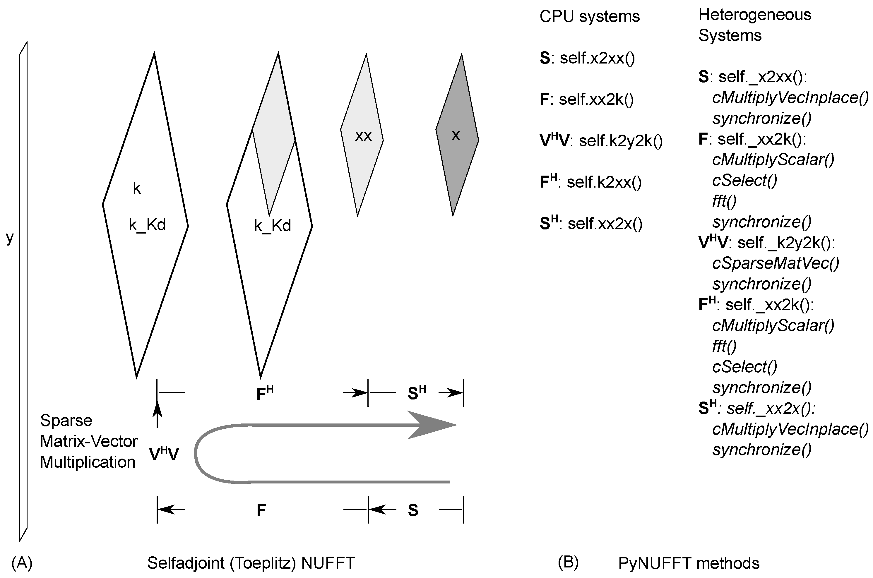
2.1.5. Self-Adjoint NUFFT (Toeplitz)
In iterative algorithms, the cost function is used to represent data fidelity:
The minimization of the cost function finds the solution at , which leads to the normal equation composed of interpolation () and gridding ():
2.2. Solver
The NUFFT provides solvers to restore multidimensional images (or one-dimensional signals in the time domain) from the non-equispaced frequency samples. A great number of reconstruction methods exist for non-Cartesian image reconstruction. These methods are usually categorized into three families: (1) density compensation and adjoint NUFFT; (2) least square regression in k-space; and (3) iterative NUFFT.
2.2.1. Density Compensation and Adjoint NUFFT
The sampling density compensation method introduces a tapering function (sampling density compensation function), which can be calculated from the following stable iterations [8]:
where the element-wise division (⊘) compensates for the over-estimation or under-estimation of the current , and . It is noted that the element-wise division tends to make the denominator closer to one. Once is prepared, the sampling density compensation method can be calculated by:
Here, the element-wise multiplication operator ⊙ multiplies the data () by the sampling density compensation function ().
2.2.2. Least Square Regression
Least square regression is a solution to the inverse problem of image reconstruction. Consider the following problem:
The solution is estimated from the above minimization problem. Due to the enormous memory requirements of the large NUFFT matrix , iterative algorithms are more frequently used.
- Conjugate gradient method (cg): For Equation (7) there is the two-step solution:Once has been solved, the inverse of can be computed by the inverse FFT and then divided by the scaling factor:The most expensive step is to find in Equation (8). The conjugate gradient method is an iterative solution when the sparse matrix is a symmetric Hermitian matrix:Then each iteration generates the residue, which is used to compute the next value. The conjugate gradient method is also provided for heterogeneous systems.
- Other iterative methods for least-squares problems: Scipy [9] provides a variety of least square solvers, including Sparse Equations and Least Squares (lsmr and lsqr), biconjugate gradient method (bicg), biconjugate gradient stabilized method (bicgstab), generalized minimal residual method (gmres), and linear solver restarted generalized minimal residual method (lgmres). These solvers are integrated into the CPU version of PyNUFFT.
2.2.3. Iterative NUFFT Using Variable Splitting
Iterative NUFFT reconstruction solves the inverse problem with various forms of image regularization. Due to the large size of the interpolation and FFT, iterative NUFFT is computationally expensive.
Here, PyNUFFT is also optimized for iterative NUFFT reconstructions in heterogeneous systems.
- Pre-indexing for fast image gradients: Total variation in basic image regularization has been extensively used in image denoising and image reconstruction. The image gradient is computed using the difference between adjacent pixels, which is represented as follows:where is the index of the i-th axis. Computing the image gradient requires image rolling, followed by a subtraction of the original image and the rolled image. However, multidimensional image rolling in heterogeneous systems is expensive and PyNUFFT adopts pre-indexing to save runtime. This pre-indexing procedure generates the indexes for the rolled image, and the indexes are offloaded to heterogeneous platforms before initiating the iterative algorithms. Thus, image rolling is not needed during the iterations. The acceleration of this pre-indexing method is demonstrated in Figure 3, in which pre-indexing makes the image gradient run faster on the CPU and GPU.
- ℓ1 total variation-regularized ordinary least square (L1TV-OLS): The ℓ1 total variation regularized reconstruction includes piece-wise smoothing into the reconstruction model.where is the total variation of the image:Here, the and are directional gradient operators applied to the image domain along the and axes. Equation (12) is solved by the variable-splitting method, which has already been developed [10,11,12].The iterations of L1TV-OLS are explicitly shown in Algorithm 1.
Algorithm 1: The pseudocode for the ℓ1 total variation-regularized ordinary least square (L1TV-OLS) algorithm ![Jimaging 04 00051 i001]()
- ℓ1 total variation-regularized least absolute deviation (L1TV-LAD): Least absolute deviation (LAD) is a statistical regression model which is robust to non-stationary noise distribution [13]. It is possible to solve the ℓ1 total variation-regularized problem with the LAD cost function [14]:where is the total variation of the image. Note that LAD is the ℓ1 norm of the data fidelity. The iterations of L1TV-LAD are as follows:Note that the shrinkage function (shrink) in Algorithm 2 can be quickly solved on the CPU as well as on heterogeneous systems.
Algorithm 2: The pseudocode for the ℓ1 total variation-regularized least absolute deviation (L1TV-LAD) ![Jimaging 04 00051 i002]()
- Multi-coil image reconstruction: In multi-coil regularized image reconstruction, the self-adjoint NUFFT in Equation (4) is extended to multi-coil data:where the coil-sensitivities () of multiple channels multiply each channel before the NUFFT () and after the adjoint NUFFT (). Sensitivity profiles can be estimated either using the magnitude of smoothed images divided by the root-mean-squared image, or using the dedicated eigenvalue decomposition method [15]. See Figure 6 for a visual example of estimation of coil sensitivity profiles.


2.2.4. Iterative NUFFT Using the Primal-Dual Type Method
In Cartesian magnetic resonance imaging (MRI), the matrix of the ℓ2 subproblem can be quickly (and exactly) solved by the diagonal matrix in the Fourier domain, i.e. the is strictly diagonal. The diagonal matrix is very convenient for compressed sensing MRI on the Cartesian grid [16]. In some non-Cartesian k-spaces, however, the matrix is not strictly diagonal, which makes variable-splitting methods prone to numerical errors. These errors may accumulate during the image reconstructions, causing instabilities.
Alternatively, the primal-dual hybrid gradient type of algorithm [17,18] exists as a simpler solution to the ℓ1-ℓ2 regularized problems. The alternative primal-dual hybrid gradient algorithms eliminate the ℓ2 subproblem, which conquers one of the major shortcomings of the ℓ1-ℓ2 problems.
- Generalized basis pursuit denoising algorithm (GBPDNA)Here, the generalized basis pursuit denoising algorithm (GBPDNA) [19] is implemented, which reads as the following Algorithm 3.In Algorithm 3, the is the NUFFT in Equation (1). are intermediate variables initiated as zeros. is the step size: . The notation is the generic regularization term, which can be the image itself (as in the fast iterative shrinkage-thresholding algorithm (FISTA) [20]), or linearly transformed images. In the next section, the total variation-like regularization terms are explicitly formulated. satisfy and .
Algorithm 3: The pseudocode for the generic generalized basis pursuit denoising algorithm (GBPDNA) algorithm ![Jimaging 04 00051 i003]() is the simple convex projection function applying to each component:is the constrained function, defined as follows:
is the simple convex projection function applying to each component:is the constrained function, defined as follows: - Matrix form of total variation-like regularizationsThe piece-wise constant total variation regularization has been used in image denoising and image reconstruction. Total generalized variation [21] introduces the piece-wise smooth model and the additional variables and to mitigate the stair-casing artifacts. Such modification allows total generalized variation to include the divergence and the curl of the image.The total variation can be written as a compact block sparse matrix. The compact form of anisotropic total variation is as follows:which yields the explicit anisotropic TV using GBPDNA:
Algorithm 4: The pseudocode for the GBPDNA algorithm for anisotropic total variation ![Jimaging 04 00051 i004]() Similarly, the explicit isotropic TV using GBPDNA is:
Similarly, the explicit isotropic TV using GBPDNA is:Algorithm 5: The pseudocode for the GBPDNA algorithm for isotropic total variation ![Jimaging 04 00051 i005]() Similar to total variation, the total generalized variation regularization can be expressed in a matrix form:where the above variables are modified to match the size of the regularization term.
Similar to total variation, the total generalized variation regularization can be expressed in a matrix form:where the above variables are modified to match the size of the regularization term.


2.3. Applications to Brain MRI
A Periodically Rotated Overlapping ParallEL Lines with Enhanced Reconstruction (PROPELLER) k-space [22] is used in the simulation study. Non-Cartesian data are retrospectively generated from a fully sampled 3T brain MRI template [23]. In conventional methods, data are regridded to a 512 × 512 k-space by linear and cubic spline interpolation methods. The gridded data are processed by IFFT. Three PyNUFFT algorithms were compared with the conventional IFFT-based method. The matrix size = 512 × 512, oversampled ratio = 2, and kernel size = 6. Parameters of L1TV-OLS and L1TV-LAD are: = 1, = 1, maximum iteration number = 500.
2.4. 3D Computational Phantom
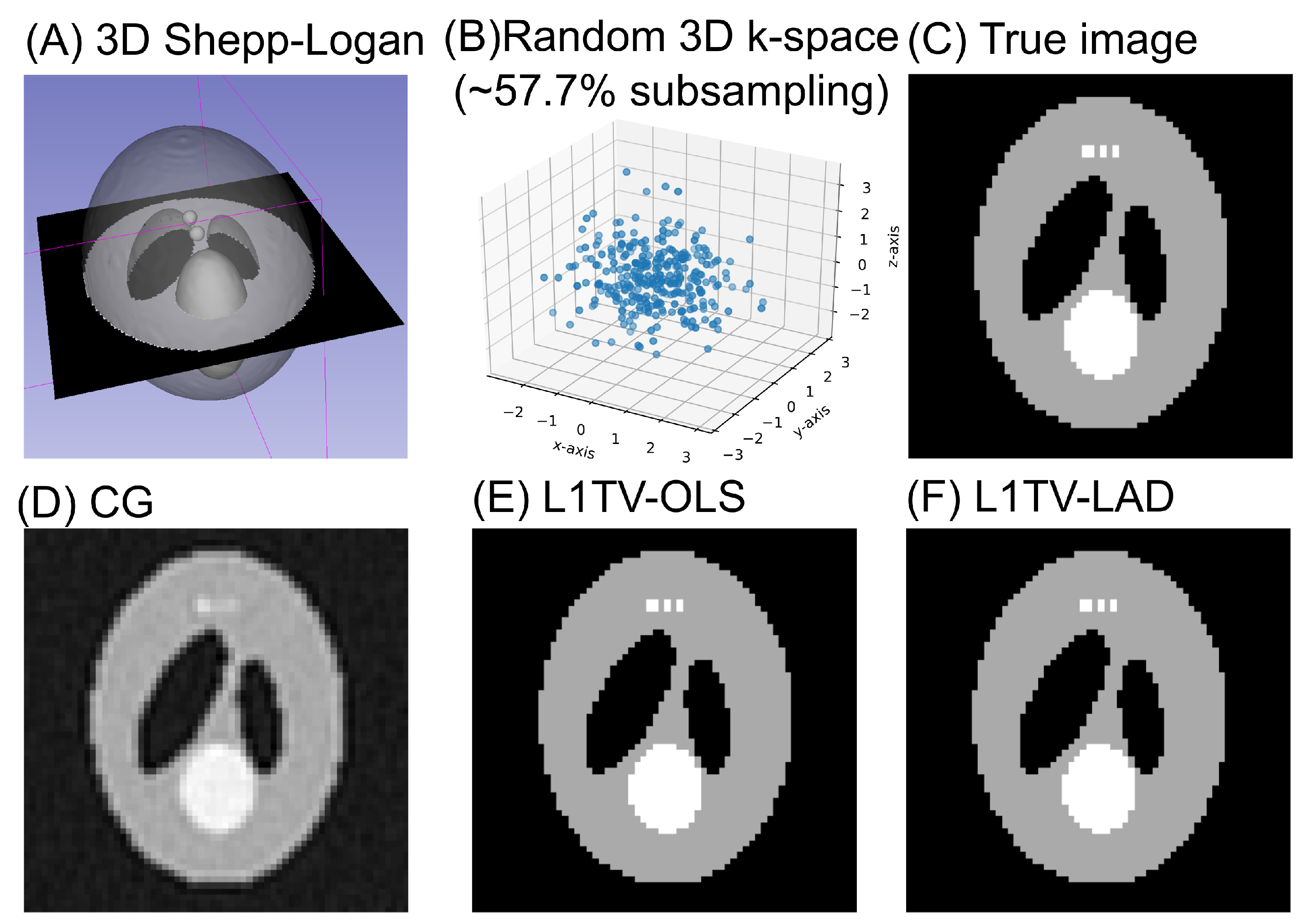
The pre-indexing mechanism of PyNUFFT allows multi-dimensional NUFFT and reconstruction to be carried out. In this simulation study, a three-dimensional (3D) computational phantom [24] (Figure 7A) was used to generate data which are randomly scattered in the 3D k-space (Figure 7B). The image parameters were: matrix size = 64 × 64 × 64, subsampling ratio = 57.7%, oversampled grid = 1×, and kernel size = 1. The parameters of L1TV-OLS and L1TV-LAD were = 1, = 0.1; the number of outer iterations was 500.
2.5. Benchmark
PyNUFFT was tested on a Linux system. All the computations were completed with a complex single precision floating point (FP32). The configurations of CPU and GPU systems were as follows.
- Multi-core CPU: The CPU instance (m4.16xlarge, Amazon Web Services) was equipped with 64 vCPUs (Intel E5 2686 v4) and 61 GB of memory. The number of vCPUs could be dynamically controlled by the CPU hotplug functionality of the Linux system, and computations were offloaded onto the Intel OpenCL CPU device with 1 to 64 threads. The single thread CPU computations were carried out with Numpy compiled with the FFTW library [25]. PyNUFFT was executed on the multi-core CPU instance with 1–64 threads. The PyNUFFT transforms were offloaded to the OpenCL CPU device and were executed 20 times. The runtimes required for the transforms were compared with the runtimes on the single-thread CPU.Iterative reconstructions were also tested on the multi-core CPU. The matrix size was 256 × 256, and kernel size was 6. The execution times of the conjugate gradient method, ℓ1 total variation regularized reconstruction and the ℓ1 total variation-regularized LAD were measured on the multi-core system.
- GPU: The GPU instance (p2.xlarge, Amazon Web Services) was equipped with 4 vCPUs (Intel E5 2686 v4) and one Tesla K80 (NVIDIA, Santa Clara, CA, USA) with two GK210 GPUs. Each GPU was composed of 2496 parallel processing cores and 12 GB of memory. Computations were preprocessed and offloaded onto one GPU by CUDA or OpenCL APIs. Computations were repeated 20 times to measure the average runtimes. The matrix size was 256 × 256, and kernel size was 6.Iterative reconstructions were also tested on the K80 GPU, and the execution times of the conjugate gradient method, ℓ1 total variation regularized reconstruction and ℓ1 total variation regularized LAD on the multi-core system were compared with the iterative solvers on the CPU with one thread.
- Comparison between PyNUFFT and Python nfft: It was previously shown that the min–max interpolator yields a better estimation of DFT than the Gaussian kernel does for a kernel size of less than 8 [4]. Thus, a similar testing was carried out and the amplitudes of 1000 randomly scattered non-uniform locations of PyNUFFT and nfft were compared to the amplitudes of the DFT. The input 1D array length was 256, and the kernel size was 2–7.The computation times of PyNUFFT and Python nfft were also measured on a single CPU core. This testing used a Linux system equipped with an Intel Core i7-6700HQ running at 2.6–3.1 GHz (Intel, Santa Clara, CA, USA) with a system memory of 16 GB.
- Comparison between PyNUFFT and gpuNUFFT : This testing used a Linux system equipped with an Intel Core i7-6700HQ running at 2.6–3.1 GHz (Intel, Santa Clara, CA, USA), 16 GB of system memory, and an NVIDIA GeForce GTX 965M (945 MHz) (NVIDIA, Santa Clara, CA, USA) with 2 GB of video memory (driver version 387.22), using the CUDA toolkit version 9.0.176. The gpuNUFFT was compiled with FP16. The parameters of the testing were: image size = 256 × 256, oversampling ratio = 2, kernel size = 6. The GPU version of PyNUFFT was executed using the identical parameters to gpuNUFFT. A radial k-space with 64 spokes [26] was used for gpuNUFFT and PyNUFFT.
- Scalability of PyNUFFT: A study of the scalability of PyNUFFT was carried out to compare the runtimes of different matrix sizes and the number of non-uniform locations. The system was equipped with a CPU (Intel Core i7 6700HQ at 3500 MHz, 16 GB system memory) and a GPU (NVIDIA GeForce GTX 965m at 945 MHz, 2 GB device memory).
3. Results
3.1. Applications to Brain MRI
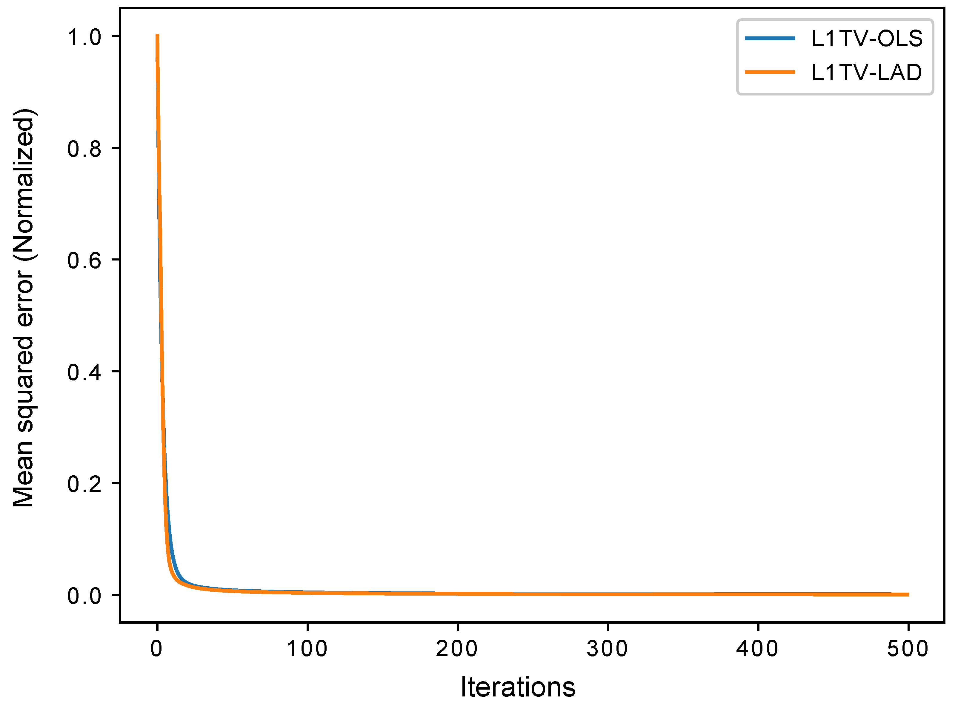
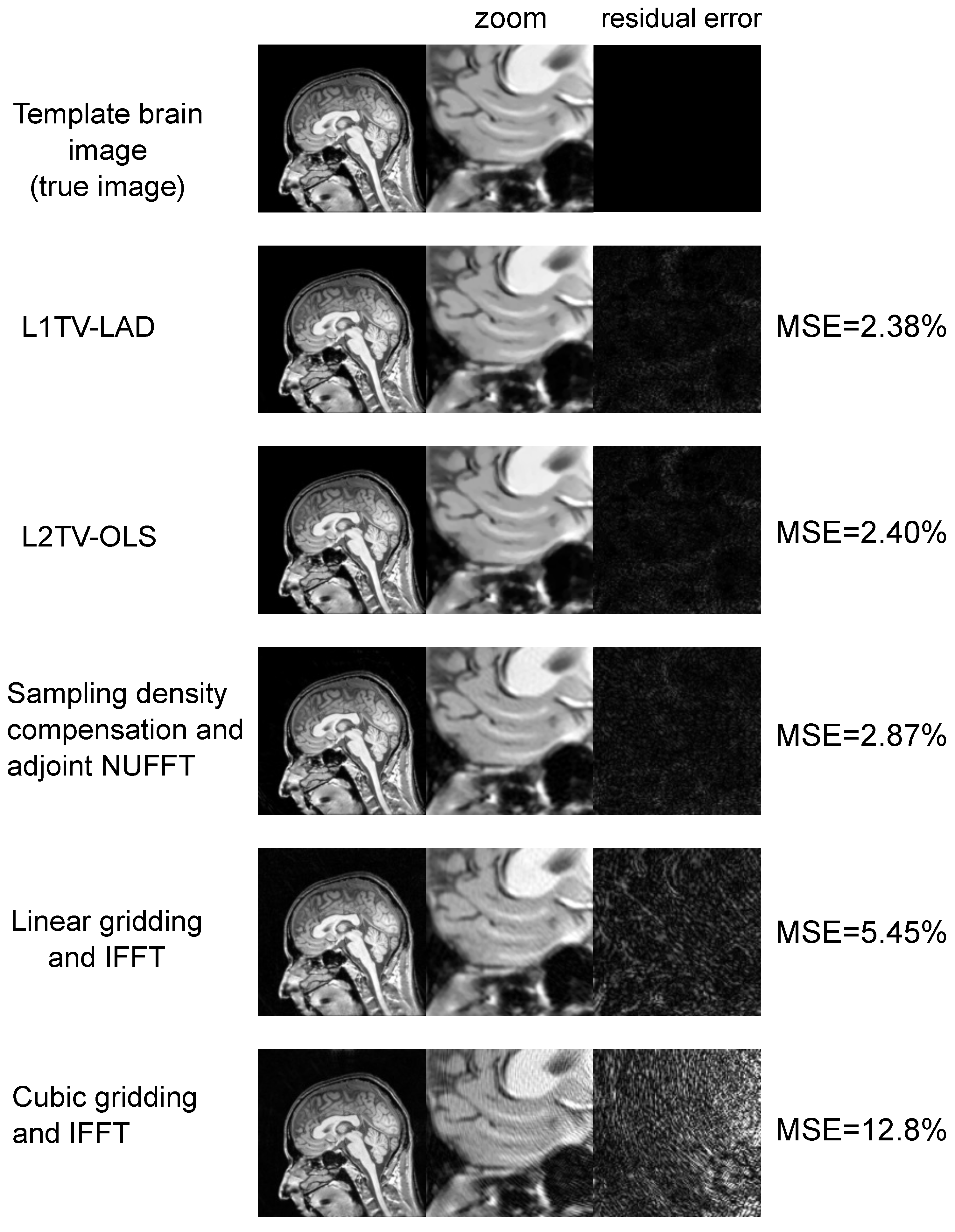
The data fidelity of L1TV-OLS and L1TV-LAD converged between 100 and 500 iterations (Figure 8). Some visual results of MRI reconstructions can be seen in Figure 9. The error of cubic spline was greater than the error (mean-squared error (MSE) = 12.8%) of linear interpolation (MSE = 5.45%). In comparison, NUFFT-based algorithms obtained lower errors than the conventional IFFT and gridding methods. Iterative NUFFT using L1TV-OLS (MSE = 2.40%) and L1TV-LAD (MSE = 2.38%) yielded fewer ripples in the brain structure than in the sampling density compensation method (MSE = 2.87%).
3.2. 3D Computational Phantom
The result of the 3D phantom study can be seen in Figure 7. While conjugate gradient (CG) generated the image volume with artifacts and blurring, ℓ1TV-OLS and ℓ1TV-LAD restored the image details and preserved the edge of the phantom.
3.3. Benchmarks
- Multi-core CPU: Table 1 lists the profile for each stage of forward NUFFT, adjoint NUFFT, and self-adjoint NUFFT (Toeplitz). The overall execution speed of PyNUFFT was faster on the multi-core CPU platform than the single-thread CPU, yet the acceleration factors of each stage varied from 0.95 (no acceleration) to 15.6. Compared with computations on a single thread, 32 threads accelerated interpolation and gridding by a factor of 12, and the FFT and IFFT were accelerated by a factor of 6.2–15.6.The benefits of 32 threads are limited for certain computations, including scaling, rescaling, and interpolation gridding (). In these computations, the acceleration factors of 32 threads range from 0.95 to 1.85. This limited performance gain is due to the high efficiency of single-thread CPUs, which leaves limited room for improvement. In particular, the integrated interpolation gridding () is already 10 times faster than the separate interpolation and regridding sequence. On a single-thread CPU, requires only 4.79 ms, whereas the separate interpolation () and gridding () require 49 ms. In this case, 32 threads only deliver an extra 83% of performance to .Figure 10 illustrates the acceleration on the multi-core CPU against the single thread CPU. The performance of PyNUFFT improved by a factor of 5–10 when the number of threads increased from 1 to 20, and the software achieved peak performance with 30–32 threads (equivalent to 15–16 physical CPU cores). More than 32 threads seem to bring no substantial improvement to the performance.Forward NUFFT, adjoint NUFFT and self-adjoint NUFFT (Toeplitz) were accelerated on 32 threads with an acceleration factor of 7.8–9.5. The acceleration factors of iterative solvers (conjugate gradient method, L1TV-OLS and L1TV-LAD) were from 4.2–5.
- GPU: Table 1 shows that GPU delivers a generally faster PyNUFFT transform, with the acceleration factors ranging from 2 to 31.Scaling and rescaling have led to a moderate degree of acceleration. The most significant acceleration took place in the interpolation-gridding () in which GPU was 26–31 times faster than single-thread CPU. This significant acceleration was faster than the acceleration factors for separate interpolation (, with 6× acceleration) and gridding ( with 4–4.6× acceleration).Forward NUFFT, adjoint NUFFT and self-adjoint NUFFT (Toeplitz) were accelerated on K80 GPU by 5.4–13. Iterative solvers on GPU were 6.3–8.9 faster than single-thread, and about twice as fast as with 32 threads.
- Comparison between PyNUFFT and Python nfft: A comparison between PyNUFFT and nfft (Figure 11) evaluated (1) the accuracy of the min–max interpolator and the Gaussian kernel; and (2) the runtimes of a single-core CPU. The min–max interpolator in PyNUFFT attains a lower error than Gaussian kernel. PyNUFFT also requires less CPU times than nfft, due to the fact that nfft recalculates the interpolation matrix with each nfft or nfft_adjoint call.
- Comparison between PyNUFFT and gpuNUFFT: Figure 12 compares the runtimes of different GPU implementations. In forward NUFFT, the fastest is the PyNUFFT (batch), followed by PyNUFFT (loop) and gpuNUFFT.In single-coil adjoint NUFFT, the performance of PyNUFFT (loop), PyNUFFT (batch) and gpuNUFFT is similar. Multi-coil NUFFT increases the runtimes, and the PyNUFFT (loop) is the slowest in the adjoint transform in the case of three coils.
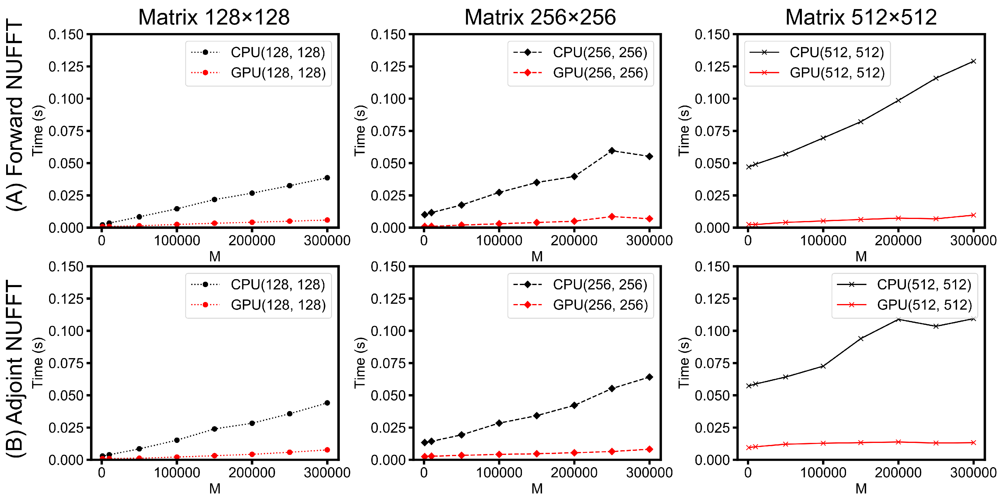
- Scalability of PyNUFFT: Figure 13 evaluates the performance of forward NUFFT and adjoint NUFFT vs. the number of non-uniform locations (M) for different matrix sizes. The condition of M = 300,000 is close to a fully sampled 512 × 512 k-space (with 262,144 samples). The values at M = 0 (y-intercept ) indicate the runtimes for scaling () and FFT (), which change with the matrix size. The slope can be attributed to the runtimes versus M, which is due to interpolation () or gridding ().For a large problem size (matrix size = 512 × 512, M = 300,000), GPU PyNUFFT requires less than 10 ms in the forward transform, and less than 15 ms in the adjoint transform. For a small problem size (matrix size = 128 × 128, M = 1000), GPU PyNUFFT requires 830 ns in the forward transform, and 850 ns in the adjoint transform.
4. Discussion
4.1. Related Work
Different kernel functions (interpolators) are available in previous NUFFT implementations, including: (1) the min–max interpoaltor [4]; (2) the fast radial basis functions [27,28]; (3) the least square interpolator [29]; (4) the least mean squared error interpolator [30]; (5) the fast Gaussian summation [31]; (6) the Kaiser–Bessel function [26]; and (7) the linear system transfer function or inverse reconstruction [32,33].
The NUFFTs have been implemented in different programming languages: (1) MATLAB (Mathworks Inc., MA, USA) [4,26,30,34]; (2) C++ [35]; (3) CUDA [26,35]; (4) Fortran [31]; and (5) OpenACC using a PGI compiler (PGI Compilers & Tools, NVIDIA Corporation, Beaverton, OR, USA) [36]. Several Python implementations of NUFFT came to our attention during the preparation of this manuscript. There are one-dimensional non-equispaced fast Fourier transform (nfft package in pure Python) and the multidimensional Python nfft (Python wrapper of the nfft C-library). A python based MRI reconstruction toolbox (mripy) based on nfft was accelerated using the Numba compiler. NUFFT has been accelerated on single and multiple GPUs. Fast iterative NUFFT using the Kaiser–Bessel function was accelerated on a GPU with total variation regularization [35] and total generalized variation regularization [26]. A real-time inverse reconstruction was developed in Sebastinan et al. [37] and Murphy et al. [38], as a pre-gridding procedure saves interpolation and gridding during iterations. The patent of Nadar et al. [39] describes a custom multi-GPU buffer to improve the memory access for image reconstruction with a non-uniform k-space.
4.2. Discussions of PyNUFFT
The current PyNUFFT has the advantage of high portability between different hardware and software systems. The NUFFT transforms (forward, adjoint, and Toeplitz) have been accelerated on multi-core CPUs and GPUs. In particular, the benefits of fast iterative solvers (including least square and iterative NUFFT) have been shown in the results of benchmarks. The image reconstruction times (with 100 iterations) for one 256 × 256 image are less than 4 s on a 32-thread CPU platform and less than 2 s on a GPU platform.
The current PyNUFFT has been tested with computations using single precision floating numbers (FP32). However, the number of double precision floating point (FP64) units on the GPU is only a fraction of the number of FP32 units, which reduces the performance with FP64 and slows down the performance of PyNUFFT.
In the future, a GPU NUFFT library written in pure C would allow researchers to use the power hardware accelerators in different high-level languages. However, the innate complexity of heterogeneous platforms tends to lower the portability of software, which results in considerable efforts for development and testing. Recently, computer scientists have proposed several emerging GPGPU initiatives to simplify the task, such as the Low Level Virtual Machine (LLVM), OpenACC, and OpenMP 4.0, and these standards are likely to mature in the next few years.
5. Conclusions
An open-source PyNUFFT package was implemented to accelerate the non-Cartesian image reconstruction on multi-core CPU and GPU platforms. The acceleration factors were 6.3–9.5× on a 32-thread CPU platform and 5.4–13× on a Tesla K80 GPU. The iterative solvers with 100 iterations could be completed within 4 s on the 32-thread CPU platform and within 2 s on the GPU.
Supplementary Materials
Part of the source code is available online at https://github.com/jyhmiinlin/pynufft.
Acknowledgments
The author acknowledges the open-source MATLAB NUFFT software [4], which is essential for the development of PyNUFFT. The author thanks Ciuciu and the research group at Neurospin, CEA, Paris, France for their inspirational suggestions about the Chambolle–Pock and Condat–Vu algorithms, which will be included in the future release of PyNUFFT. This work was supported by the Ministry of Science and Technology, Taiwan (in 2016–2017), partially by the Cambridge Commonwealth, European and International Trust, Cambridge, UK, and the Ministry of Education, Taiwan (2012–2016). The benchmarks were carried out on Amazon Web Services provided by Educate credit.
Author Contributions
The author developed the PyNUFFT in 2012–2018. Since 2016, PyNUFFT has been re-engineered to improve its runtime efficiency.
Conflicts of Interest
The author received an NVIDIA GPU grant. The founding sponsors had no role in the design of the study; in the collection, analyses, or interpretation of data; in the writing of the manuscript, and in the decision to publish the results.
Abbreviations
The following abbreviations are used in this manuscript:
| CG | conjugate gradient |
| CPU | central processing unit |
| CPU | central processing unit |
| DFT | discrete Fourier transform |
| GBPDNA | generalized basis pursuit denoising algorithm |
| GPU | graphic processing unit |
| IFFT | inverse fast Fourier transform |
| MRI | magnetic resonance imaging |
| MSE | mean squared error |
| NUFFT | non-uniform fast Fourier transform |
| TV | total variation |
References
- Klöckner, A.; Pinto, N.; Lee, Y.; Catanzaro, B.; Ivanov, P.; Fasih, A. PyCUDA and PyOpenCL: A scripting-based approach to GPU run-time code generation. Parallel Comput. 2012, 38, 157–174. [Google Scholar] [CrossRef]
- Opanchuk, B. Reikna, A Pure Python GPGPU Library. Available online: http://reikna.publicfields.net/ (accessed on 9 October 2017).
- Free Software Foundation. GNU General Public License. 29 June 2007. Available online: http://www.gnu.org/licenses/gpl.html (accessed on 7 March 2018).
- Fessler, J.; Sutton, B.P. Nonuniform fast Fourier transforms using min-max interpolation. IEEE Trans. Signal Proc. 2003, 51, 560–574. [Google Scholar] [CrossRef]
- Danalis, A.; Marin, G.; McCurdy, C.; Meredith, J.; Roth, P.; Spafford, K.; Tipparaju, V.; Vetter, J. The Scalable HeterOgeneous Computing (SHOC) Benchmark Suite. In Proceedings of the 3rd Workshop on General-Purpose Computation on Graphics Processors (GPGPU 2010), Pittsburgh, PA, USA, 14 March 2010. [Google Scholar]
- Knuth, D.E. The Art of Computer Programming, Volume 1 (3rd ed.): Fundamental Algorithms; Addison Wesley Longman Publishing Co., Inc.: Redwood City, CA, USA, 1997. [Google Scholar]
- Fessler, J.; Lee, S.; Olafsson, V.T.; Shi, H.R.; Noll, D.C. Toeplitz-based iterative image reconstruction for MRI with correction for magnetic field inhomogeneity. IEEE Trans. Signal Proc. 2005, 53, 3393–3402. [Google Scholar] [CrossRef]
- Pipe, J.G.; Menon, P. Sampling density compensation in MRI: Rationale and an iterative numerical solution. Magn. Reson. Med. 1999, 41, 179–186. [Google Scholar] [CrossRef]
- Jones, E.; Oliphant, T.; Peterson, P. SciPy: Open source scientific tools for Python. 2001. Available online: http://www.scipy.org (accessed on 9 October 2017).
- Lin, J.M.; Patterson, A.J.; Chang, H.C.; Chuang, T.C.; Chung, H.W.; Graves, M.J. Whitening of Colored Noise in PROPELLER Using Iterative Regularized PICO Reconstruction. In Proceedings of the 23rd Annual Meeting of International Society for Magnetic Resonance in Medicine, Toronto, ON, Canada, 30 May–5 June 2015; p. 3738. [Google Scholar]
- Lin, J.M.; Patterson, A.J.; Lee, C.W.; Chen, Y.F.; Das, T.; Scoffings, D.; Chung, H.W.; Gillard, J.; Graves, M. Improved Identification and Clinical Utility of Pseudo-Inverse with Constraints (PICO) Reconstruction for PROPELLER MRI. In Proceedings of the 24th Annual Meeting of International Society for Magnetic Resonance in Medicine, Singapore, 7–13 May 2016; p. 1773. [Google Scholar]
- Lin, J.M.; Tsai, S.Y.; Chang, H.C.; Chung, H.W.; Chen, H.C.; Lin, Y.H.; Lee, C.W.; Chen, Y.F.; Scoffings, D.; Das, T.; et al. Pseudo-Inverse Constrained (PICO) Reconstruction Reduces Colored Noise of PROPELLER and Improves the Gray-White Matter Differentiation. In Proceedings of the 25th Annual Meeting of International Society for Magnetic Resonance in Medicine, Honolulu, HI, USA, 22–28 April 2017; p. 1524. [Google Scholar]
- Wang, L. The penalized LAD estimator for high dimensional linear regression. J. Multivar. Anal. 2013, 120, 135–151. [Google Scholar] [CrossRef]
- Lin, J.M.; Chang, H.C.; Chao, T.C.; Tsai, S.Y.; Patterson, A.; Chung, H.W.; Gillard, J.; Graves, M. L1-LAD: Iterative MRI reconstruction using L1 constrained least absolute deviation. In Proceedings of the 34th Annual Scientific Meeting of ESMRMB, Barcelona, Spain, 19–21 October 2017. [Google Scholar]
- Uecker, M.; Lai, P.; Murphy, M.J.; Virtue, P.; Elad, M.; Pauly, J.M.; Vasanawala, S.S.; Lustig, M. ESPIRiT-an eigenvalue approach to autocalibrating parallel MRI: Where SENSE meets GRAPPA. Magn. Reson. Med. 2014, 71, 990–1001. [Google Scholar] [CrossRef] [PubMed]
- Goldstein, T.; Osher, S. The split Bregman method for ℓ1-regularized problems. SIAM J. Imaging Sci. 2009, 2, 323–343. [Google Scholar] [CrossRef]
- Chambolle, A.; Pock, T. A first-order primal-dual algorithm for convex problems with applications to imaging. J. Math. Imaging Vis. 2011, 40, 120–145. [Google Scholar] [CrossRef]
- Boyer, C.; Ciuciu, P.; Weiss, P.; Mériaux, S. HYR2PICS: Hybrid Regularized Reconstruction for Combined Parallel Imaging and Compressive Sensing in MRI. In Proceedings of the 9th IEEE International Symposium on Biomedical Imaging (ISBI), Barcelona, Spain, 2–5 May 2012; pp. 66–69. [Google Scholar]
- Loris, I.; Verhoeven, C. Iterative algorithms for total variation-like reconstructions in seismic tomography. GEM Int. J. Geomath. 2012, 3, 179–208. [Google Scholar] [CrossRef]
- Beck, A.; Teboulle, M. A fast iterative shrinkage-thresholding algorithm for linear inverse problems. SIAM J. Imaging Sci. 2009, 2, 183–202. [Google Scholar] [CrossRef]
- Knoll, F.; Bredies, K.; Pock, T.; Stollberger, R. Second order total generalized variation (TGV) for MRI. Magn. Reson. Med. 2011, 65, 480–491. [Google Scholar] [CrossRef] [PubMed]
- Lin, J.M.; Patterson, A.J.; Chang, H.C.; Gillard, J.H.; Graves, M.J. An iterative reduced field-of-view reconstruction for periodically rotated overlapping parallel lines with enhanced reconstruction PROPELLER MRI. Med. Phys. 2015, 42, 5757–5767. [Google Scholar] [CrossRef] [PubMed]
- Lalys, F.; Haegelen, C.; Ferre, J.C.; El-Ganaoui, O.; Jannin, P. Construction and assessment of a 3-T MRI brain template. Neuroimage 2010, 49, 345–354. [Google Scholar] [CrossRef] [PubMed] [Green Version]
- Schabel, M. MathWorks File Exchange: 3D Shepp-Logan Phantom. Available online: https://uk.mathworks.com/matlabcentral/fileexchange/9416-3d-shepp-logan-phantom (accessed on 9 October 2017).
- Frigo, M.; Johnson, S. The Design and Implementation of FFTW3. Proc. IEEE 2005, 93, 216–231. [Google Scholar] [CrossRef]
- Knoll, F.; Schwarzl, A.; Diwoky, C.S.D. gpuNUFFT—An open-source GPU library for 3D gridding with direct Matlab Interface. In Proceedings of the 22nd Annual Meeting of ISMRM, Milan, Italy, 20–21 April 2013; p. 4297. [Google Scholar]
- Potts, D.; Steidl, G. Fast summation at nonequispaced knots by NFFTs. SIAM J. Sci. Comput. 2004, 24, 2013–2037. [Google Scholar] [CrossRef]
- Keiner, J.; Kunis, S.; Potts, D. Using NFFT 3—A software library for various nonequispaced fast Fourier transforms. ACM Trans. Math. Softw. 2009, 36, 19. [Google Scholar] [CrossRef]
- Song, J.; Liu, Y.; Gewalt, S.L.; Cofer, G.; Johnson, G.A.; Liu, Q.H. Least-square NUFFT methods applied to 2-D and 3-D radially encoded MR image reconstruction. IEEE Trans. Biom. Eng. 2009, 56, 1134–1142. [Google Scholar] [CrossRef] [PubMed]
- Yang, Z.; Jacob, M. Mean square optimal NUFFT approximation for efficient non-Cartesian MRI reconstruction. J. Magn. Reson. 2014, 242, 126–135. [Google Scholar] [CrossRef] [PubMed]
- Greengard, L.; Lee, J.Y. Accelerating the nonuniform fast Fourier transform. SIAM Rev. 2004, 46, 443–454. [Google Scholar] [CrossRef]
- Liu, C.; Moseley, M.; Bammer, R. Fast SENSE Reconstruction Using Linear System Transfer Function. In Proceedings of the International Society of Magnetic Resonance in Medicine, Miami Beach, FL, USA, 7–13 May 2005; p. 689. [Google Scholar]
- Uecker, M.; Zhang, S.; Frahm, J. Nonlinear inverse reconstruction for real-time MRI of the human heart using undersampled radial FLASH. Magn. Reson. Med. 2010, 63, 1456–1462. [Google Scholar] [CrossRef] [PubMed]
- Ferrara, M. Implements 1D-3D NUFFTs Via Fast Gaussian Gridding. 2009. Matlab Central. Available online: http://www.mathworks.com/matlabcentral/fileexchange/25135-nufft-nfft-usfft (accessed on 2 March 2018).
- Bredies, K.; Knoll, F.; Freiberger, M.; Scharfetter, H.; Stollberger, R. The Agile Library for Biomedical Image Reconstruction Using GPU Acceleration. Comput. Sci. Eng. 2013, 15, 34–44. [Google Scholar]
- Cerjanic, A.; Holtrop, J.L.; Ngo, G.C.; Leback, B.; Arnold, G.; Moer, M.V.; LaBelle, G.; Fessler, J.A.; Sutton, B.P. PowerGrid: A open source library for accelerated iterative magnetic resonance image reconstruction. Proc. Intl. Soc. Mag. Reson. Med. 2016, 24, 525. [Google Scholar]
- Schaetz, S.; Voit, D.; Frahm, J.; Uecker, M. Accelerated computing in magnetic resonance imaging: Real-time imaging Using non-linear inverse reconstruction. Comput. Math. Methods Med. 2017. [Google Scholar] [CrossRef] [PubMed]
- Murphy, M.; Alley, M.; Demmel, J.; Keutzer, K.; Vasanawala, S.; Lustig, M. Fast-SPIRiT compressed sensing parallel imaging MRI: Scalable parallel implementation and clinically feasible runtime. IEEE Trans. Med. Imaging 2012, 31, 1250–1262. [Google Scholar] [CrossRef] [PubMed]
- Nadar, M.S.; Martin, S.; Lefebvre, A.; Liu, J. Multi-GPU FISTA Implementation for MR Reconstruction with Non-Uniform k-space Sampling. U.S. Patent 14/031,374, 27 March 2014. [Google Scholar]
- Stone, S.S.; Haldar, J.P.; Tsao, S.C.; Hwu, W.M.W.; Liang, Z.P.; Sutton, B.P. Accelerating Advanced MRI Reconstructions on GPUs. J. Parallel Distrib. Comput. 2008, 68, 1307–1318. [Google Scholar] [CrossRef] [PubMed]
- Gai, J.; Obeid, N.; Holtrop, J.L.; Wu, X.L.; Lam, F.; Fu, M.; Haldar, J.P.; Wen-Mei, W.H.; Liang, Z.P.; Sutton, B.P. More IMPATIENT: A gridding-accelerated Toeplitz-based strategy for non-Cartesian high-resolution 3D MRI on GPUs. J. Parallel Distrib. Comput. 2013, 73, 686–697. [Google Scholar] [CrossRef] [PubMed]
Figure 1.
(A) The Python non-uniform fast Fourier transform (PyNUFFT) source code is preprocessed and offloaded to the multi-core central processing unit (CPU) or graphic processing unit (GPU). (B) Memory hierarchy of the device. Variables are allocated on global memory, which reduces the memory transfer times between the host memory and the device. See [1] for PyCUDA and PyOpenCL.
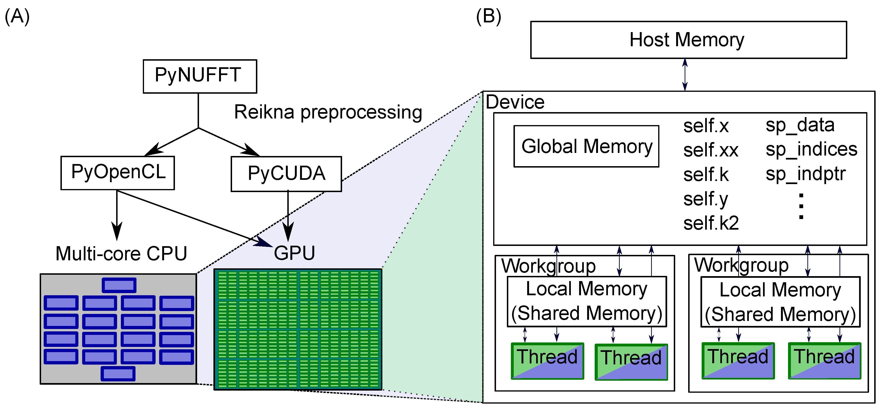
Figure 2.
(A) A two-dimensional example of the forward PyNUFFT; (B) The methods provided in PyNUFFT. Forward NUFFT can be decomposed into three stages: scaling, fast Fourier transform (FFT), and interpolation.
Figure 2.
(A) A two-dimensional example of the forward PyNUFFT; (B) The methods provided in PyNUFFT. Forward NUFFT can be decomposed into three stages: scaling, fast Fourier transform (FFT), and interpolation.
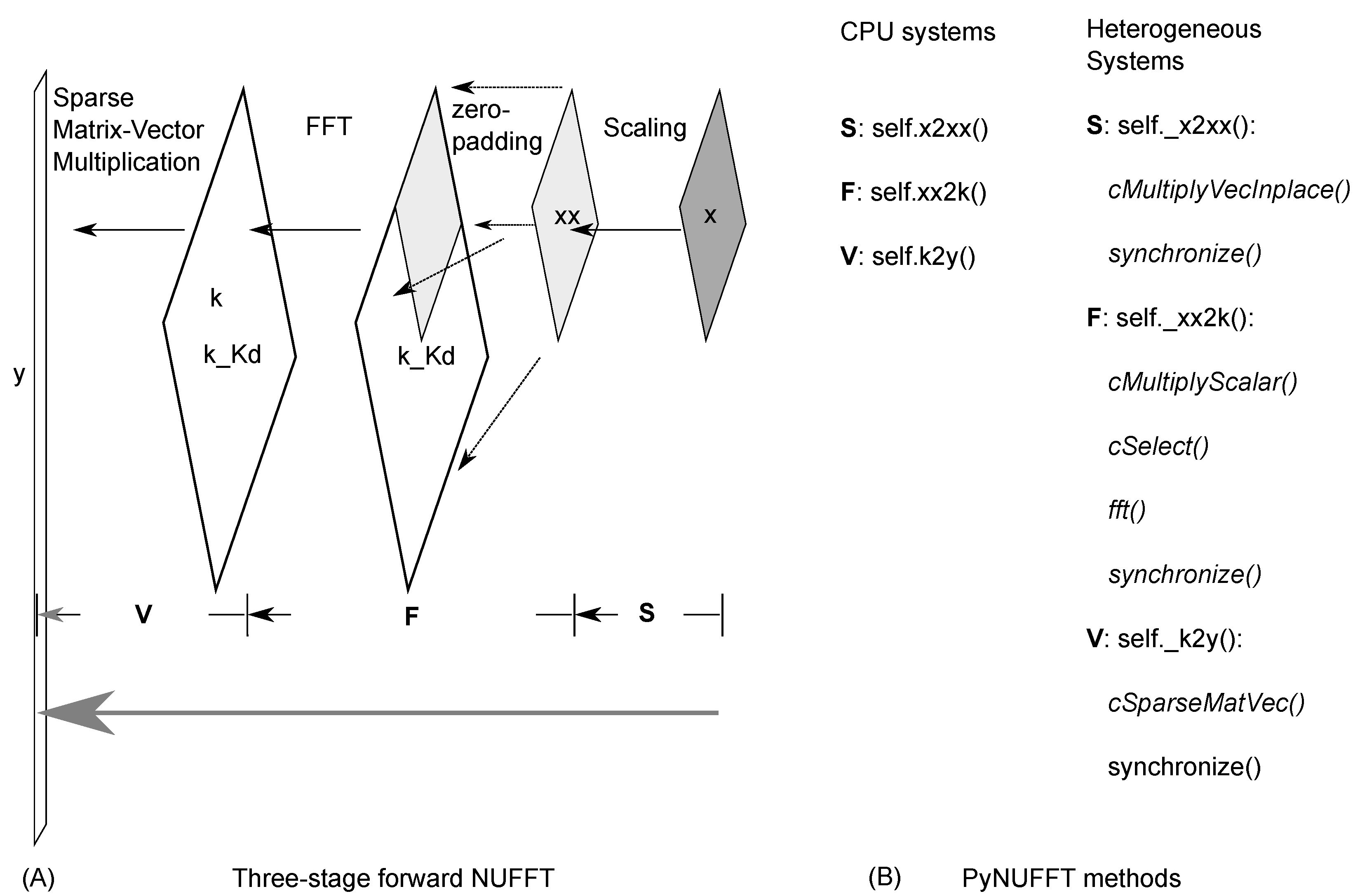
Figure 3.
Pre-indexing for the fast image gradient (∇ and ∇T). The image gradient can be slow if image rolling is to be recalculated with each iteration. Pre-indexing can save the time needed for recalculation and image gradient during iterations.
Figure 3.
Pre-indexing for the fast image gradient (∇ and ∇T). The image gradient can be slow if image rolling is to be recalculated with each iteration. Pre-indexing can save the time needed for recalculation and image gradient during iterations.

Figure 4.
(A) The adjoint PyNUFFT; (B) The methods provided in PyNUFFT. Adjoint NUFFT can be decomposed into three stages: gridding, inverse FFT (IFFT), and rescaling.
Figure 4.
(A) The adjoint PyNUFFT; (B) The methods provided in PyNUFFT. Adjoint NUFFT can be decomposed into three stages: gridding, inverse FFT (IFFT), and rescaling.
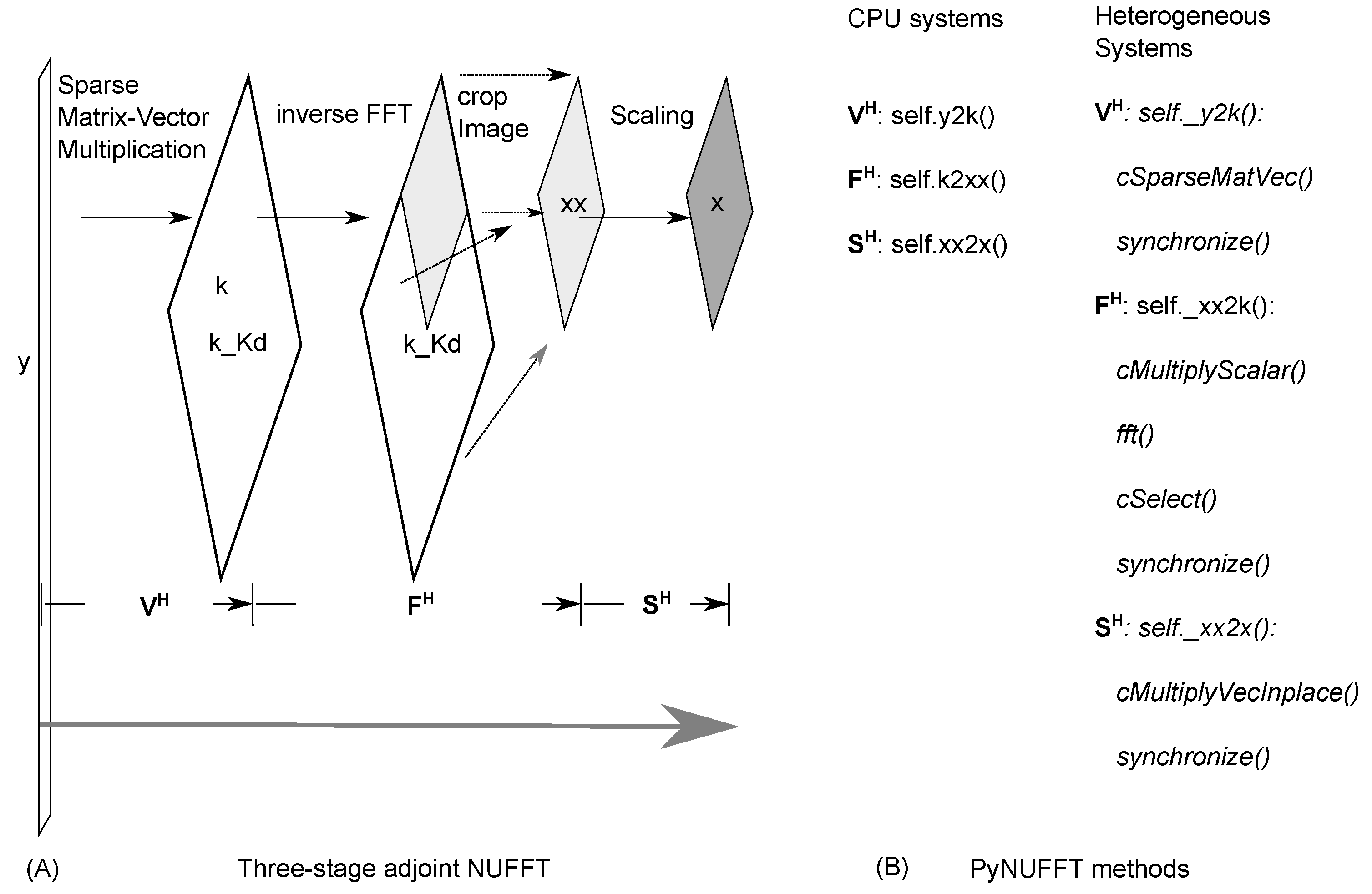
Figure 5.
(A) The self-adjoint NUFFT (Toeplitz); (B) The methods are provided in PyNUFFT. The Toeplitz method precomputes the interpolation-gridding matrix (VHV), which can be accelerated on the CPU and GPU. See Table 1 for measured acceleration factors.
Figure 5.
(A) The self-adjoint NUFFT (Toeplitz); (B) The methods are provided in PyNUFFT. The Toeplitz method precomputes the interpolation-gridding matrix (VHV), which can be accelerated on the CPU and GPU. See Table 1 for measured acceleration factors.

Figure 6.
An example of multi-coil sensitivity profiles estimated by the eigenvalue approach [15]. (A) Simulated sensitivity profiles. (B) Images from multi-channel. (C) Sensitivity profiles estimated from (B).
Figure 6.
An example of multi-coil sensitivity profiles estimated by the eigenvalue approach [15]. (A) Simulated sensitivity profiles. (B) Images from multi-channel. (C) Sensitivity profiles estimated from (B).
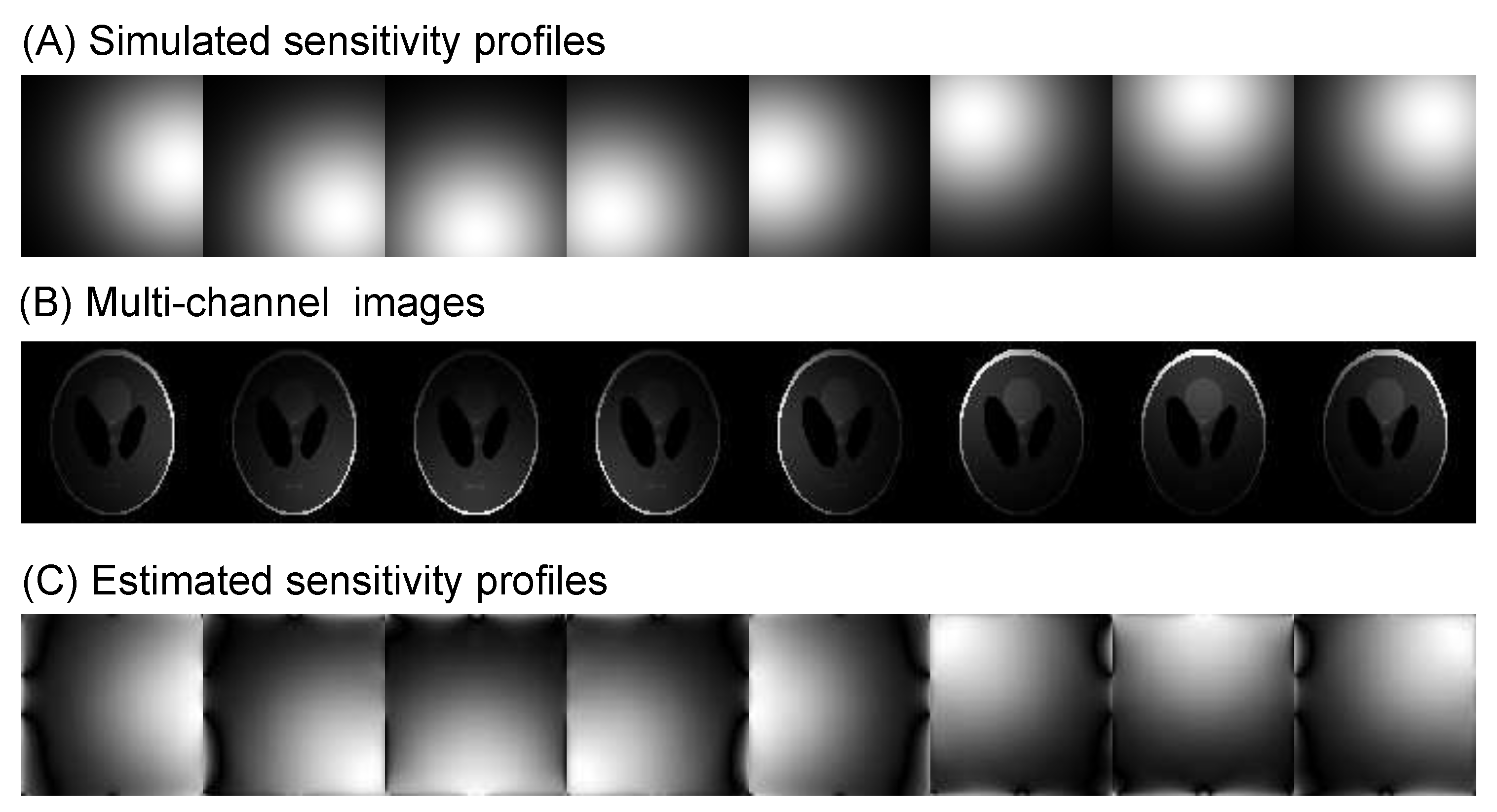
Figure 7.
Simulated results of a 3D phantom. (A) The volume rendering of the 3D phantom. The cutting plane is set to visually compare the original (C) and restored image volumes (D–F). (B) The random non-Cartesian 3D k-space (sampling ratio = 57.7%). (C) The true image. (D) Image reconstructed by the conjugate gradient (CG) method. (E) L1TV-OLS; (F) L1TV-LAD.

Figure 8.
The mean squared error (MSE) of two iterative NUFFT algorithms—L1TV-OLS and L1TV-LAD—which converge within 500 iterations.
Figure 8.
The mean squared error (MSE) of two iterative NUFFT algorithms—L1TV-OLS and L1TV-LAD—which converge within 500 iterations.

Figure 9.
Simulated results of brain magnetic resonance imaging (MRI). A Periodically Rotated Overlapping ParallEL Lines with Enhanced Reconstruction (PROPELLER) k-space [22] was used in the simulated study. Matrix size = 512 × 512, oversampled ratio = 2, kernel size = 6, maximum iteration number = 500. The brain template was reconstructed with L1TV-OLS and L1TV-LAD, the sampling density compensation method, and two gridding-based IFFT methods. Compared with sampling density compensation method, fewer ripples can be seen in L1TV-OLS and L1TV-LAD. The conventional IFFT combined with two gridding methods caused a greater MSE than the iterative NUFFT algorithms.

Figure 10.
Acceleration factors against the number of virtual CPUs (vCPUs). Optimal performance occurs around 30–32 threads. There is no substantial benefit from more than 32 vCPUs.
Figure 10.
Acceleration factors against the number of virtual CPUs (vCPUs). Optimal performance occurs around 30–32 threads. There is no substantial benefit from more than 32 vCPUs.
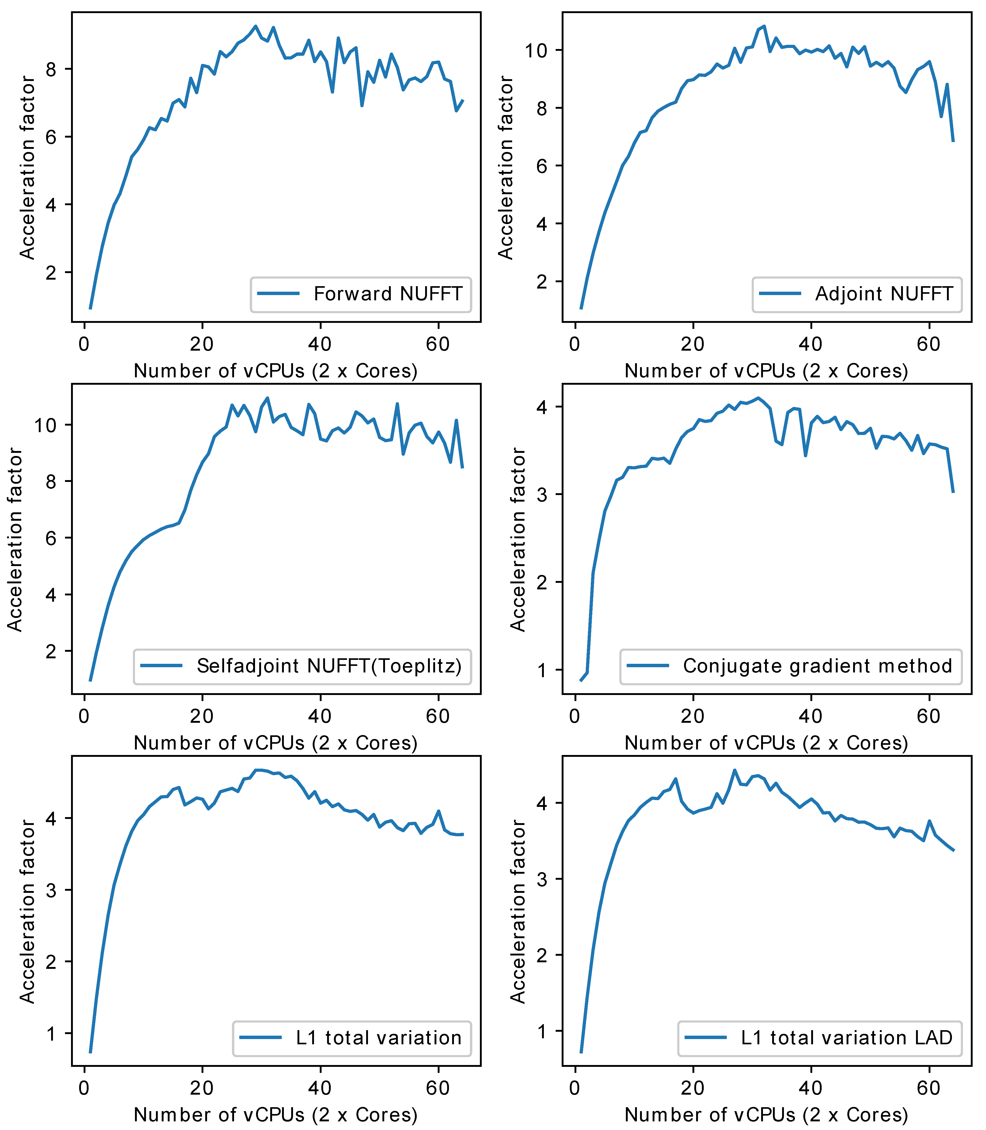
Figure 11.
(A) The errors of the min–max interpolator (in PyNUFFT) and the Gaussian kernel (in Python nfft). The parameters are: one-dimensional (1D) case, 1000 non-uniform locations, grid size = 256, oversampling factor = 2, FFT size = 512. (B) The runtimes of PyNUFFT and Python nfft on a single CPU core (Intel Core i7 6700HQ at 3500 MHz, 16 GB system memory). The Numpy was compiled with FFTW3 in the tests.
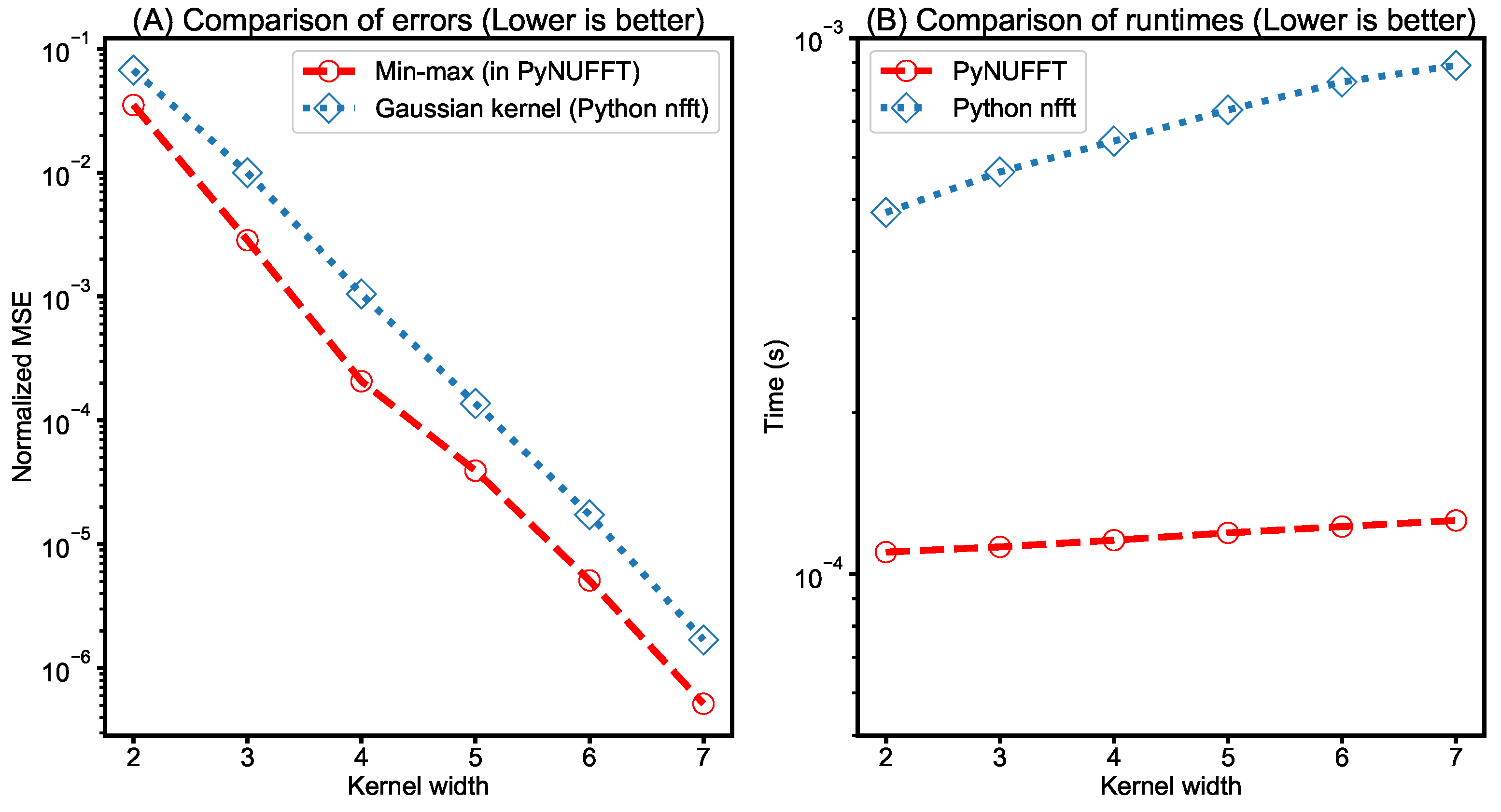
Figure 12.
(A) Runtimes of forward transform in PyNUFFT (loop), PyNUFFT (batch mode) and gpuNUFFT (B) Runtimes of adjoint transform in PyNUFFT (loop), PyNUFFT (batch mode) and gpuNUFFT. The batch-mode PyNUFFT requires a large device memory, which is proportional to the number of coils. The benchmark used a radial k-space with 64 spokes in the test file in Knoll et al. [26]. NVIDIA GeForce 965 m with 945 MHz and 2 GB device memory is used as the GPU. The parameters of the test are: image size = 256 × 256, oversampling ratio = 2, kernel size = 6.
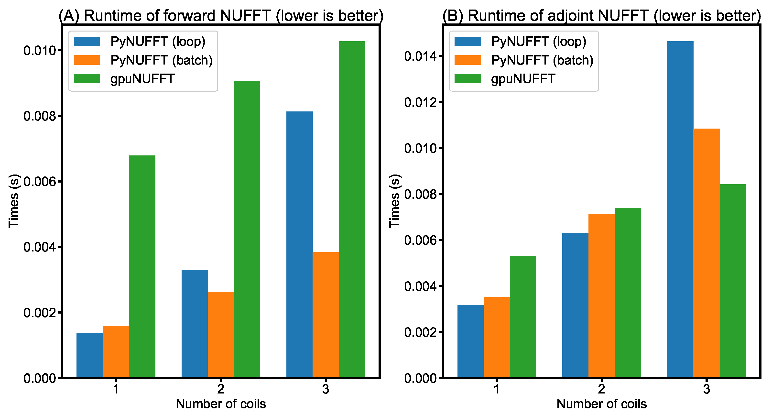
Figure 13.
Runtimes versus the number of non-uniform locations (M) for different matrix sizes. (A) Forward NUFFT; (B) Adjoint NUFFT. The system was equipped with a CPU (Intel Core i7 6700HQ at 3500 MHz, 16 GB system memory) and a GPU (NVIDIA GeForce GTX 965 m, 945 MHz, 2 GB device memory).
Figure 13.
Runtimes versus the number of non-uniform locations (M) for different matrix sizes. (A) Forward NUFFT; (B) Adjoint NUFFT. The system was equipped with a CPU (Intel Core i7 6700HQ at 3500 MHz, 16 GB system memory) and a GPU (NVIDIA GeForce GTX 965 m, 945 MHz, 2 GB device memory).

Table 1.
The runtime and acceleration (shown in parentheses) of subroutines and solvers.
| Operations | 1 vCPU * | 32 vCPUs | PyOpenCL K80 | PyCUDA K80 |
|---|---|---|---|---|
| Scaling(S) | 709 µs | 557 µs (1.3×) | 133 µs (5.3×) | 300 µs (2.4×) |
| FFT(F) | 12.6 ms | 2.03 ms (6.2×) | 0.78 ms (16.2×) | 1.12 ms (11.3×) |
| Interpolation(V) | 25 ms | 2 ms (12×) | 4 ms(6×) | 4 ms (6×) |
| Gridding(VH) | 24 ms | 2 ms (12×) | 5 ms (4.8×) | 4.5 ms (5.4×) |
| IFFT(FH) | 16 ms | 3.1 ms (5.16×) | 4.0 ms (4×) | 3.5 (4.6×) |
| Rescaling (SH) | 566 µs | 595 µs (0.95×) | 122 µs (4.64×) | 283 µs (2×) |
| VHV | 4.79 ms | 2.62 ms (1.83×) | 0.18 ms (26×) | 0.15 ms (31×) |
| Forward (A) | 39 ms | 5 ms (7.8×) | 6 ms (6.5×) | 6 ms (6.5×) |
| Adjoint (AH) | 38 ms | 6 ms (6.3×) | 7 ms (5.4×) | 6 ms (6.3×) |
| Self-adjoint (AHA) | 34.7 ms | 11 ms (3.15×) | 9 ms (3.86×) | 8 ms (4.34×) |
| Solvers | 1 vCPU | 32 vCPUs | PyOpenCL K80 | PyCUDA K80 |
| Conjugate gradient | 11.8 s | 2.97 s (4×) | 1.32 s (8.9×) | 1.89 s (6.3×) |
| L1TV-OLS | 14.7 s | 3.26 s (4.5×) | 1.79 s (8.2×) | 1.68 s (8.7×) |
| L1TV-LAD | 15.1 s | 3.62 s (4.2×) | 1.93 s (7.8×) | 1.78 s (8.5×) |
* vCPU: virtual CPU.
© 2018 by the author. Licensee MDPI, Basel, Switzerland. This article is an open access article distributed under the terms and conditions of the Creative Commons Attribution (CC BY) license (http://creativecommons.org/licenses/by/4.0/).
Share and Cite
MDPI and ACS Style
Lin, J.-M. Python Non-Uniform Fast Fourier Transform (PyNUFFT): An Accelerated Non-Cartesian MRI Package on a Heterogeneous Platform (CPU/GPU). J. Imaging 2018, 4, 51. https://doi.org/10.3390/jimaging4030051
AMA Style
Lin J-M. Python Non-Uniform Fast Fourier Transform (PyNUFFT): An Accelerated Non-Cartesian MRI Package on a Heterogeneous Platform (CPU/GPU). Journal of Imaging. 2018; 4(3):51. https://doi.org/10.3390/jimaging4030051
Chicago/Turabian StyleLin, Jyh-Miin. 2018. "Python Non-Uniform Fast Fourier Transform (PyNUFFT): An Accelerated Non-Cartesian MRI Package on a Heterogeneous Platform (CPU/GPU)" Journal of Imaging 4, no. 3: 51. https://doi.org/10.3390/jimaging4030051
Note that from the first issue of 2016, this journal uses article numbers instead of page numbers. See further details here.