An Investigation of Smooth TV-Like Regularization in the Context of the Optical Flow Problem


Department of Mathematics, College of Science, King Khalid University, Abha 61421, Saudi Arabia
†
On leave from Cadi Ayyad University, ENSA Marrakech 40000, Morocco.
J. Imaging 2018, 4(2), 31; https://doi.org/10.3390/jimaging4020031
Submission received: 28 November 2017
/
Revised: 24 January 2018
/
Accepted: 26 January 2018
/
Published: 31 January 2018
Abstract
:Total variation (TV) is widely used in many image processing problems including the regularization of optical flow estimation. In order to deal with non differentiability of the TV regularization term, smooth approximations have been considered in the literature. In this paper, we investigate the use of three known smooth TV approximations, namely: the Charbonnier, Huber and Green functions. We establish the maximum theoretical error of these approximations and discuss their performance evaluation when applied to the optical flow problem.
1. Introduction
TV-based optical flow can be cast into the following form:
where is the optical flow, is a data energy function, is the norm, and is a regularization parameter weighting the relative importance of data and smoothing terms. Although the TV semi-norm has been useful for performing edge-preserving regularization [1,2,3,4,5,6,7,8,9], it is known to be numerically difficult to handle. Despite its convexity, it is not linear, quadratic or even everywhere-differentiable. Thus, the non-smoothness of this term prevents a straightforward application of gradient based optimization methods.
To remedy the problem of non-differentiability of the norm function , there are two solutions. First, we can split where and for . The norm of x will be then equal to , which will remove non-differentiability at zero but unfortunately the problem dimension will be doubled and the optimization will become constrained since y and z should be positive. The second remedy, which we are investigating in this paper, is to replace the norm by a smooth approximation.
Any smooth TV regularization should address two issues: (1) It should remove the singularities that are caused by the use of TV regularization; (2) It should maintain the preservation of motion boundaries. Several smooth approximations of the norm have been established in the literature for the regularization of a wide variety of problems [10,11,12,13,14,15,16,17], as well as for the optical flow problem [2,3,4,5].
To our knowledge, there is no theory that establishes optimality of any of these approximations; the best choice is application dependent. For instance, Nikolova and Ng [17] have considered different smooth TV approximations in the context of restoration and reconstruction of images and signals using half quadratic minimization. Our objective in this paper is to investigate the use of three known smooth TV approximations, namely: the Charbonnier, Huber and Green functions for the case of optical flow computation.
The outline of this paper is as follows. Section 2 describes the variational formulation of the optical flow problem. In particular, we present the TV regularization model for dense optical flow estimation. In Section 3, we consider three smooth approximations of the TV regularization term and discuss their maximum theoretical error of approximation. Section 4 concerns the performance evaluation of the three approximations in terms of the quality of the estimated optical flow and the speed of convergence by using the Middlebury datasets. Finally, we conclude our work in Section 5.
2. Variational Formulation
Let us consider a sequence of gray level images , , , where is the temporal domain and denotes the image spatial domain. We will use both continuous and disc in time at frame numbers , and in space at pixel coordinates , with m (respectively n) corresponds to the discrete column (respectively row) of the image, being the coordinate origin located in the top-left corner of the image. With this notation, denotes a discrete representation of . We will also use both continuous and quantized image intensities and the same symbol I will be used for both of them.
Assuming that the gray level of a point does not change over time we may write the constraint
where is the apparent trajectory of the point . Taking the derivative with respect to t and denoting , we obtain the linear optical flow constraint
The vector field is called optical flow and , denote the temporal and spatial partial derivatives of I, which are computed using high-pass gradient filters for discrete images. Clearly, the single constraint (2) is not sufficient to uniquely compute the two components of the optical flow (this is called the aperture problem) and only gives the component of the flow normal to the image gradient, i.e., to the level lines of the image. As it is usual, in order to recover a unique flow field, some prior knowledge about it should be added. For that, we assume that the optical flow varies smoothly in space, or better, that is piecewise smooth in . This can be achieved by including a smoothness term of the form
where is a suitable function.
Both data attachment (1) and regularization term (3) can be combined into a single energy functional
where the data functional D is either equal to the linear term
or the nonlinear term
and is a regularization parameter.
When using the linear data term (5), the case corresponds to the Horn-Schunck model [18] and the case , where , corresponds to the Nagel-Enkelmann model [19]. On the other hand, the TV regularization [1] became the most used in image processing because it allows for discontinuities preserving. In this case, for , we have
where is the space of infinitely differentiable vector-valued functions with compact support. Note that when , the distributional derivative of w is a vector-valued Radon measure with total variation . When , the TV semi-norm reduces to the -norm of the gradient so that
where we can have either or . We have chosen the first one because the Euclidean norm is known to be rotationally invariant.
For a full account of regularization techniques for the optical flow problem and the associated taxonomy, we refer to [20,21].
In this paper, we will consider a TV regularization model which is written in the discrete form as follows:
where and is a set of neighbors of the pixel p. We will also combine the TV regularization with the nonlinear data term (6) used with a robust function in order to remove outliers:
The robust function used in this paper is
where is a given threshold.
3. Smooth TV Regularization
In this section, we focus on approximating the non-smooth TV semi-norm (7) by a smooth function:
where is a smooth approximation of the absolute value function and is a small parameter adjusting the accuracy of this approximation. In this paper, we will consider variants choices of as illustrated in Table 1.
Notice that the regularization term in (9) with a function from Table 1 is a hybrid between the TV regularization (7) and the standard quadratic regularization [18]. It takes the form of a quadratic or nearly quadratic for small values of the optical flow gradient and becomes linear or sublinear for large values of the optical flow gradient. In this way, this smooth regularization will retain the fast Laplacian diffusion inside homogeneous motion regions and its effect is substantially reduced near motion boundaries helping the preservation of these boundaries’ edges. We should also note that the smaller the parameter is, the better the function approximates the absolute value function; and henceforth the better the smooth regularization (9) approximates the TV regularization (7). In practice, a very small parameter might cause numerical instabilities but such a choice is not really needed as the quadratic regularization is preferred inside homogeneous regions.
According to the discussion above, there are minimum conditions that should satisfy any approximation (see [10]):
By simple calculus, it can be shown that the approximations we are considering in this paper, which are given in Table 1, satisfy the conditions in (10). Notice also that all these approximations are suitable for 1st order numerical convex optimization algorithms since they are all convex and differentiable. However, for 2nd order numerical optimization algorithms, the Charbonnier and Green functions are twice differentiable but the Huber function is not. In this case, the latter approximation is normally replaced by a twice differentiable function called the pseudo Huber approximation [12], which is the same as the Charbonnier function except for a vertical translation by .
3.1. Charbonnier Approximation
The first approximation
is referred to as the Charbonnier penalty function [11]. It was first used for optical flow in [5]. This function is clearly strictly convex and infinitely differentiable. Moreover, we can easily prove that it approximates the absolute value function with an error at most equal to .
Lemma 1.
For , where is the Charbonnier function (11).
The Charbonnier TV regularization is therefore an approximation of the TV regularization of order . Let be the total number of image pixels and be the fixed size of each neighborhood which is used for the finite difference approximation of the optical flow gradient.
Proposition 1.
, where in is the Charbonnier function (11).
Proof.
Using the previous lemma, we get
☐
3.2. Huber Approximation
The Huber function
was initially used by Huber (see [13]) as an M-estimator in the field of robust statistics. Its use for optical flow computation was first discussed in [2]. Later, it was used as a smooth approximation of the norm as in [16]. The Huber function is clearly convex and continuously differentiable.
We want to relate the Huber regularization in (9) to the TV and quadratic regularization. First, the following lemma shows that the Huber function approximates the absolute function with an error of order .
Lemma 2.
For , where is the Huber function (12).
Proof.
Let . Suppose first that . Hence
Now, if , then ☐
This shows that the Huber TV regularization has a maximum theoretical error twice better than that of the Charbonnier TV regularization.
Proposition 2.
, where in is the Huber function (12).
3.3. Green Approximation
The Green penalty function
was originally used in [14] for the maximum likelihood reconstruction from emission tomography data as a convex extension of the Geman and McClure function [15]. This penalty function was introduced for optical flow computation in [3,4]. Again, this function is strictly convex and infinitely differentiable inheriting these properties from the log cosh function. Notice that we have translated the original Green function by a factor , which is the maximum approximation error as shown by the following lemma.
Lemma 3.
For , where is the Green function (13).
Proof.
Let . First, we have
Hence, for , we have Now, if , then
Therefore, whatever the sign of s, we get
☐
The Green TV regularization approximates the TV regularization with an order as well but the maximum error is slightly greater than that of the Huber TV regularization.
Proposition 3.
, where in is the Green function (13).
4. Experimental Results
We want to minimize the energy functional (4) where D is given by (8), R is given by (9) and is one of the smooth approximations presented in the previous section. We choose to adopt the discretize-optimize approach by applying a numerical optimization algorithm to this discrete version of the optical flow minimization problem. The problem is of a large-scale type and therefore we solve it using a multiresolution line search truncated Newton method as developed in [22,23]. The method first builds a pyramid of images at different levels of resolution. It starts then at the coarsest level with a zero flow field and applies a number of iterations of the line search truncated Newton (LSTN) algorithm. Afterwards, the obtained coarse estimation is taken to the next fine level by bilinear interpolation. This process is repeated until reaching the finest level where a good initial estimate of the optical flow is obtained and henceforth refined by the LSTN algorithm until convergence is reached.
The parameter , present in the data term and which is shared by the three functionals, was fixed to a value between ten and twenty depending on the nature of the image sequence. However, in order to have a fair comparison, the parameters and involved in the regularization term yielding a different energy functional, are tuned for each functional to have the best results. From the experiments, we have noticed that functionals with the Charbonnier and Huber approximations will share in general the same set of optimal parameters. As expected the set of optimal parameters for the Green function is different, especially for the value of since the function has a different transition level between its quadratic and linear parts.
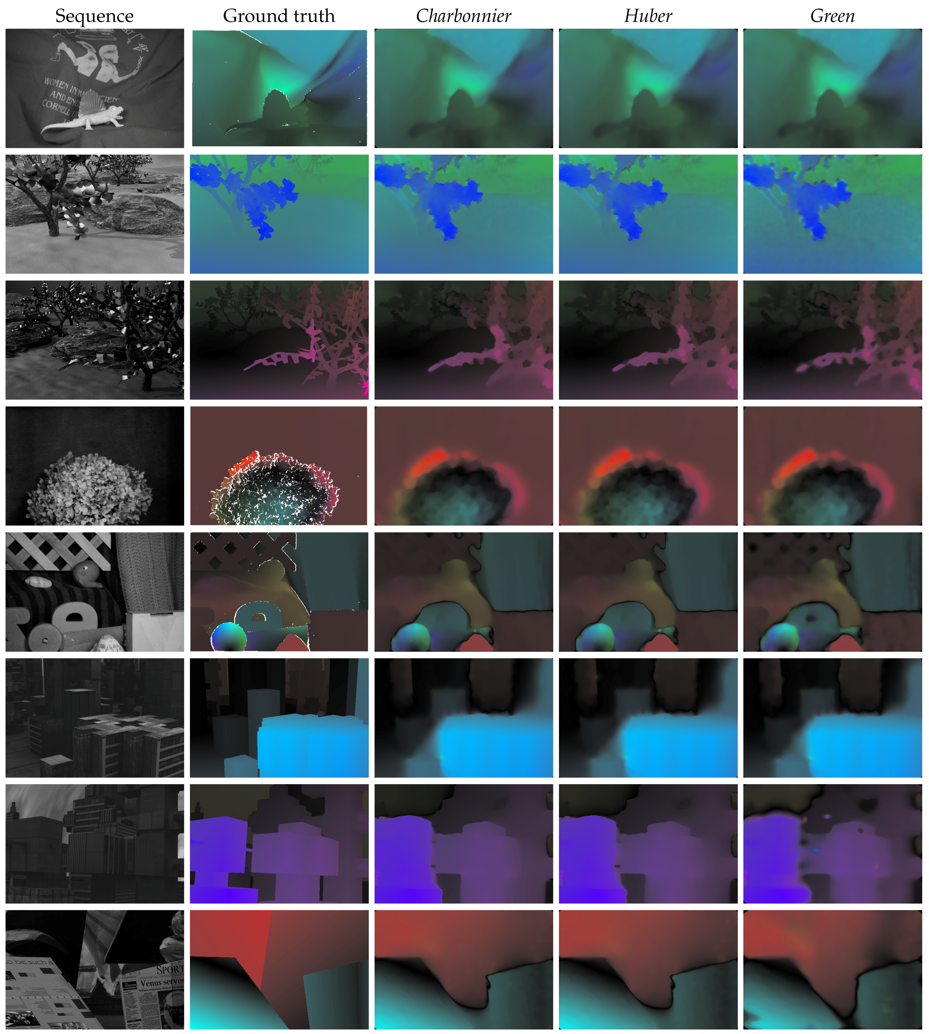
In Figure 1, we show the colored based representation of the ground truth and the best optical flow estimates obtained using Charbonnier, Huber and Green smooth TV regularizations for the Middlebury training benchmark [24] using the best parameters. Notice first how the motion boundaries are preserved for all images in Figure 1. This is indeed a famous property of the TV regularization that has been inherited by its three smooth approximations. In Figure 2, we present other tested image sequences that have different types of movement. The first three images have a translation of different sizes: half, one and ten for the spiral, peppers and band sequences, respectively. The baboon sequence has a rotation movement and the Lena sequence has a homography mapping. These five images are standard test images in image processing that have been used as the first frames and the second frames have been generated by applying the movements described above. The Marble blocks sequence, which has a zoom transformation, was obtained from the Image Sequence Server, Institut für Algorithmen und Kognitive Systeme, (Group Prof. Dr. H.-H. Nagel), University of Karlsruhe, Germany and was first used in [25]. Finally, the rotating sphere sequence was generated by the Computer Vision Research Group at the University of Otago, New Zealandand the book sequence by the Computer Laboratory at Cambridge University.
Table 2 and Table 3 present the performance comparison of the three approximations in terms of the quality of the optical flow estimation measured by the average angular error (AAE) and the average endpoint error (AEE). In Table 4, we give also the interpolation error measured by the displaced frame difference (DFD), which corresponds to the data term in the energy functional (4). Then in Table 5, we provide a comparison with respect to the speed of convergence given by the number of gradient evaluations (Ng).
First, we remark that the Charbonnier and Huber approximations lead to similar results with a slight preference for the latter. Globally, these two approximations perform better than the Green TV regularization in terms of both the average angular error and the average endpoint error of the estimated optical flow solution, and the speed of convergence as shown in Table 6. On a total of sixteen image sequences, Huber method has performed better half of the time in terms of AEE with an average of 3.836 per image sequence. It has also 9 times a better AEE with an average of 0.468. The method needs an average of 466 gradient evaluations to reach the estimated solution. This is slightly better than Charbonnier method, which has averages of 3.849, 0.469 and 473 for AAE, AEE and Ng, respectively. Nevertheless, the Green approximation has the best performance with respect to the interpolation error. The method has performed better on thirteen image sequences out of sixteen with an average DFD of 0.580 per sequence; while Charbonnier and Huber approximations have an average DFD of 0.670 and 0.678, respectively. On the other hand, Green method has better AAE and three different sequences, better AEE for two sequences, and better Ng for four sequences.
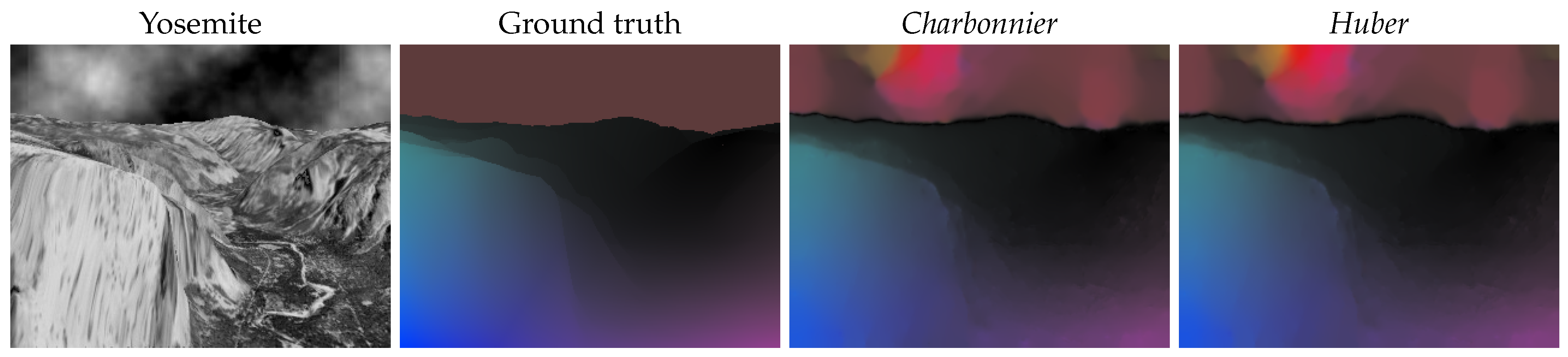
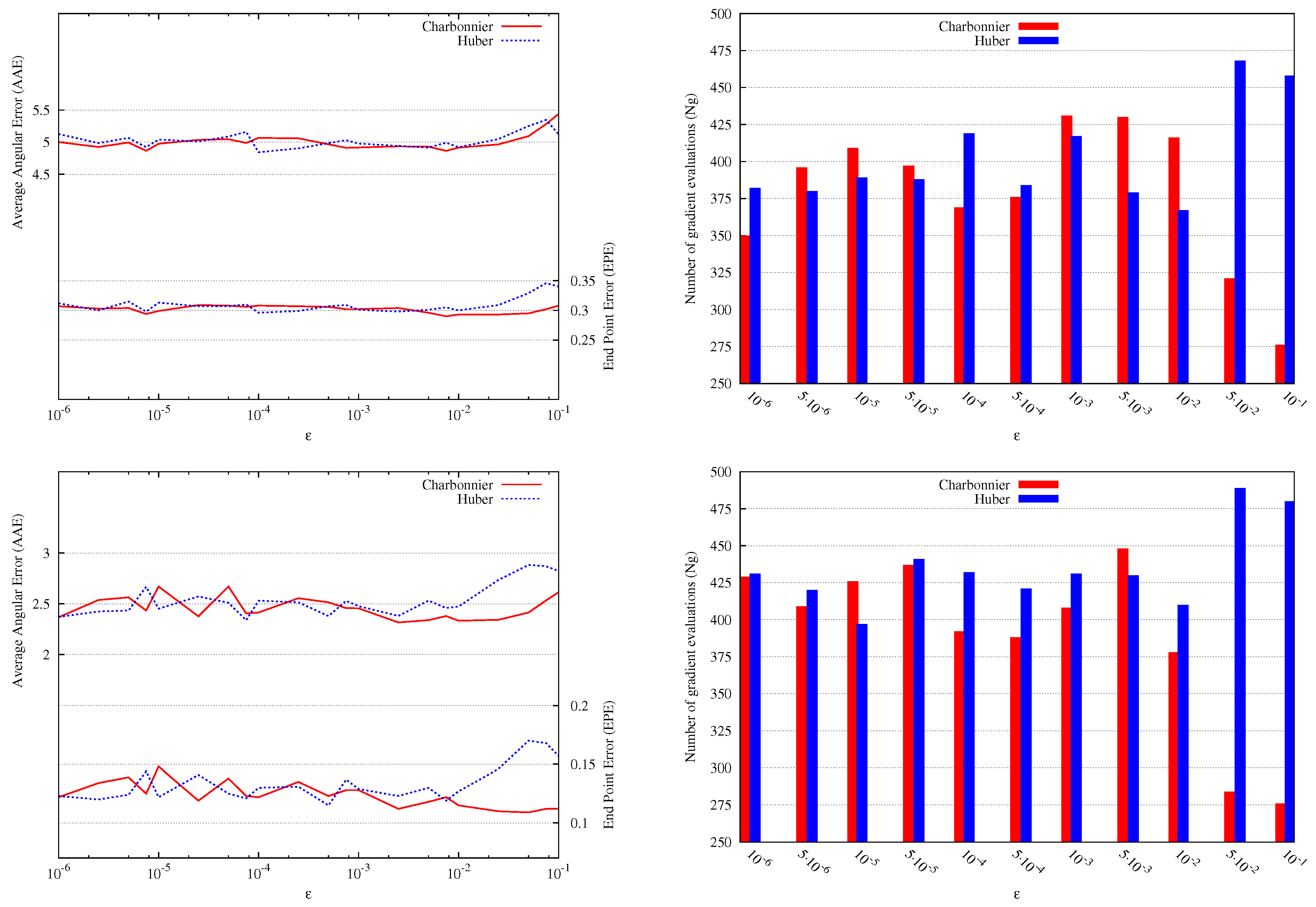
We have noticed also that the Green method is very sensitive to the parameter , which is due to the sensitivity of the hyperbolic function cosh to roundoff errors. The Charbonnier and Huber approximations suffer less from this problem. This might explain their wide use as smooth TV approximations in image processing. In Figure 3, we show the dependence of the estimated solution on the parameter for these two approximations using the Yosemite sequence, which was created by Lynn Quam at SRI and first used for optical flow in [26]. The dependence is shown in terms of AAE, AEE and Ng. For the Yosemite sequence with clouds, we can see that both the Charbonnier and Huber TV approximations give similar results for values of between and . For , Charbonnier approximation is slightly better than Huber approximation but the latter is performing better for values of around . Otherwise, the two approximations are performing almost the same except for large values of near where Charbonnier gives slightly better AEE but Huber has better AAE. In Figure 4 and Table 7, the results are shown using the best parameters.
5. Conclusions
We have investigated the use of three smooth approximations of the TV regularization in the context of the optical flow problem. We have used the same non linear data optical flow term and the same multilevel truncated Newton algorithm for the three approximations. On sixteen tested image sequences, the Huber function has confirmed its best theoretical approximation with an overall better performance in terms of both the quality of the estimated optical flow and the speed of convergence. Although the Charbonnier function has the worst theoretical approximation, it has performed almost the same as the Huber function and better than the Green function. On the other hand, in terms of the interpolation error, the Green function appears to be the best method. It has performed better on thirteen images out of sixteen.
Acknowledgments
This work was supported by the program of research support in King Khalid University under contract G.R.P-92-38. The support does not include any funds for covering the costs to publish in open access. The author would like to thank the two anonymous referees for their valuable comments and suggestions that contributed to improving the final version of the paper.
Conflicts of Interest
The author declares no conflict of interest. The founding sponsors had no role in the design of the study; in the collection, analyses, or interpretation of data; in the writing of the manuscript, and in the decision to publish the results.
References
- Rudin, L.; Osher, S.; Fatemi, E. Nonlinear total variation based noise removal algorithms. Physica D 1992, 60, 259–268. [Google Scholar] [CrossRef]
- Shulman, D.; Herve, J.-Y. Regularization of discontinuous flow fields. In Proceedings of the IEEE Workshop on Visual Motion, Irvine, CA, USA, 20–22 March 1989; pp. 81–86. [Google Scholar]
- Rouchouze, B.; Mathieu, P.; Gaidon, T.; Barlaud, M. Motion estimation based on markov random fields. In Proceedings of the 1st IEEE International Conference on Image Processing, Austin, TX, USA, 13–16 November 1994; pp. 270–274. [Google Scholar]
- Deriche, R.; Kornprobst, P.; Aubert, G. Optical-flow estimation while preserving its discontinuities: A variational approach. In Proceedings of the Asian Conference on Computer Vision, Singapore, 5–8 December 1995; pp. 69–80. [Google Scholar]
- Bruhn, A.; Weickert, J.; Schnörr, C. Lucas/Kanade meets Horn/Schunck: Combining local and global optic flow methods. Int. J. Comput. Vis. 2005, 61, 211–231. [Google Scholar] [CrossRef]
- Zach, C.; Pock, T.; Bischof, H. A duality based approach for realtime TV-L 1 optical flow. In Proceedings of the 29th DAGM Conference on Pattern Recognition, Heidelberg, Germany, 12–14 September 2007; pp. 214–223. [Google Scholar]
- Chambolle, A.; Pock, T. A first-order primal-dual algorithm for convex problems with applications to imaging. J. Math. Imaging Vis. 2011, 40, 120–145. [Google Scholar] [CrossRef]
- Ranftl, R.; Bredies, K.; Pock, T. Non-local total generalized variation for optical flow estimation. In Proceedings of the European Conference on Computer Vision, Zurich, Switzerland, 6–12 September 2014; pp. 439–454. [Google Scholar]
- Ali, S.; Daul, C.; Galbrun, E.; Blondel, W. Illumination invariant optical flow using neighborhood descriptors. Comput. Vis. Image Underst. 2016, 145, 95–110. [Google Scholar] [CrossRef]
- Aubert, G.; Kornprobst, P. Mathematical Problems in Image Processing: Partial Differential Equations and the Calculus of Variations; Springer Science & Business Media: New York, NY, USA, 2006. [Google Scholar]
- Charbonnier, P.; Blanc-Féraud, L.; Aubert, G.; Barlaud, M. Deterministic edge-preserving regularization in computed imaging. IEEE Trans. Image Process. 1997, 6, 298–311. [Google Scholar] [CrossRef] [PubMed]
- Hartley, R.; Zisserman, A. Multiple View Geometry in cOmputer Vision; Cambridge University Press: Cambridge, MA, USA, 2003. [Google Scholar]
- Huber, P.J. Robust Statistics; Springer: New York, NY, USA, 2011. [Google Scholar]
- Green, P.J. Bayesian reconstructions from emission tomography data using a modified EM algorithm. IEEE Trans. Med. Imaging 1990, 9, 84–93. [Google Scholar] [CrossRef] [PubMed]
- Geman, S.; McClure, D. Bayesian image analysis: An application to single photon emission tomography. In Proceedings of the Statistical Association Section, Las Vegas, Nevada, 5–8 August 1985; pp. 12–18. [Google Scholar]
- Madsen, K.; Nielsen, H.B. A finite smoothing algorithm for linear l_1 estimation. SIAM J. Optim. 1993, 3, 223–235. [Google Scholar] [CrossRef]
- Nikolova, M.; Ng, M.K. Analysis of half-quadratic minimization methods for signal and image recovery. SIAM J. Sci. Comput. 2005, 27, 937–966. [Google Scholar] [CrossRef]
- Horn, B.; Schunk, B. Determining optical flow. Artif. Intell. 1981, 17, 185–203. [Google Scholar] [CrossRef]
- Nagel, H.-H.; Enkelmann, W. An investigation of smoothness constraints for the estimation of displacement vector fields from image sequences. IEEE Trans. Pattern Anal. Mach. Intell. 1986, 8, 565–593. [Google Scholar] [CrossRef] [PubMed]
- Weickert, J.; Schnorr, C. A theoretical framework for convex regularizers in PDE-based computation of image motion. Int. J. Comput. Vis. 2001, 45, 245–264. [Google Scholar] [CrossRef]
- Hinterberger, W.; Scherzer, O.; Schnörr, C.; Weickert, J. Analysis of optical flow models in the framework of the calculus of variations. Numer. Funct. Anal. Optim. 2002, 23, 69–89. [Google Scholar] [CrossRef]
- Kalmoun, E.M.; Garrido, L.; Caselles, V. Line search multilevel optimization as computational methods for dense optical flow. SIAM J. Imaging Sci. 2011, 4, 695–722. [Google Scholar] [CrossRef] [Green Version]
- Garrido, L.; Kalmoun, E.M. A line search multilevel truncated Newton algorithm for computing the optical flow. Image Process. Line 2015, 124–138. [Google Scholar] [CrossRef]
- Baker, S.; Scharstein, D.; Lewis, J.P.; Roth, S.; Black, M.J.; Szeliski, R. A database and evaluation methodology for optical flow. Int. J. Comput. Vis. 2011, 92, 1–31. [Google Scholar] [CrossRef]
- Otte, M.; Nagel, H.H. Estimation of optical flow based on higher-order spatiotemporal derivatives in interlaced and non-interlaced image sequences. Artif. Intell. 1995, 78, 5–43. [Google Scholar] [CrossRef]
- Heeger, D. Model for the extraction of image flow. J. Opt. Soc. Am. A Opt. Image Sci. Vis. 1987, 4, 1455–1471. [Google Scholar] [CrossRef]
Figure 1.
Optical flow estimates with best parameters using Charbonnier, Huber and Green TV regularizations for the Middlebury images [24] ordered as in Table 2.

Figure 2.
Other image sequences that are used in the comparison tables.
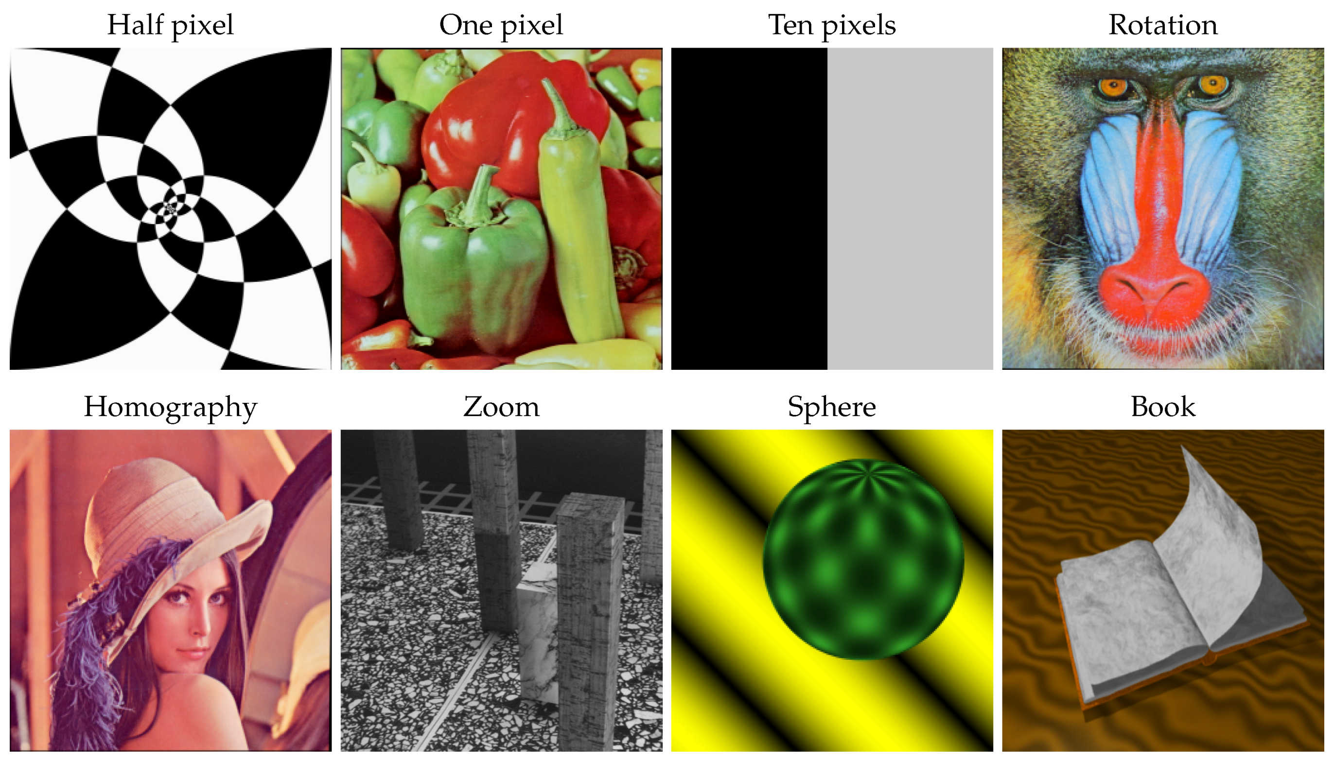
Figure 3.
Sensitivity of Charbonnier and Huber TV regularizations for the Yosemite sequence with clouds (top) and without clouds (bottom) with respect to the choice of . On the left, we show the quality of the estimated optical flow in terms of AAE and AEE . On the right, we compare the number of gradient evaluations. and . The x-axis is log scaled.

Figure 4.
Optical flow estimates with best parameters using Charbonnier and Huber TV regularizations for the Yosemite sequence.
Figure 4.
Optical flow estimates with best parameters using Charbonnier and Huber TV regularizations for the Yosemite sequence.

Table 1.
Smooth approximations of the absolute value function and their derivatives. The graphs of these approximations are plotted versus the absolute value function near zero for .
Table 1.
Smooth approximations of the absolute value function and their derivatives. The graphs of these approximations are plotted versus the absolute value function near zero for .
| Charbonnier | Huber | Green |
|---|---|---|
 |  |  |
Table 2.
Average Angular Error (AAE) using Charbonnier, Huber and Green TV regularizations for the Middlebury datasets (top) and the image sequences given in Figure 2 in the same order (bottom).
Table 2.
Average Angular Error (AAE) using Charbonnier, Huber and Green TV regularizations for the Middlebury datasets (top) and the image sequences given in Figure 2 in the same order (bottom).
| Dimetrodon | Grove2 | Grove3 | Hydrangea | Rubberwhale | Urban2 | Urban3 | Venus | |
|---|---|---|---|---|---|---|---|---|
| Charbonnier | 2.561 | 2.736 | 6.857 | 3.335 | 6.629 | 6.657 | 7.209 | 8.085 |
| Huber | 2.562 | 2.716 | 6.819 | 3.364 | 6.632 | 6.579 | 7.288 | 8.083 |
| Green | 2.539 | 2.899 | 7.333 | 3.179 | 6.979 | 6.490 | 8.433 | 8.400 |
| 1/2 Pixel | 1 Pixel | 10 Pixels | Rotation | Homography | Zoom | Sphere | Book | |
| Charbonnier | 2.412 | 0.307 | 0.009 | 0.794 | 2.724 | 6.981 | 3.525 | 0.773 |
| Huber | 2.382 | 0.308 | 0.006 | 0.767 | 2.668 | 6.901 | 3.588 | 0.715 |
| Green | 6.519 | 0.299 | 0.200 | 1.779 | 2.872 | 7.480 | 3.830 | 1.531 |
Table 3.
Average Endpoint Error (AEE) using Charbonnier, Huber and Green TV regularizations for the Middlebury datasets (top) and the image sequences given in Figure 2 in the same order (bottom).
Table 3.
Average Endpoint Error (AEE) using Charbonnier, Huber and Green TV regularizations for the Middlebury datasets (top) and the image sequences given in Figure 2 in the same order (bottom).
| Dimetrodon | Grove2 | Grove3 | Hydrangea | Rubberwhale | Urban2 | Urban3 | Venus | |
|---|---|---|---|---|---|---|---|---|
| Charbonnier | 0.139 | 0.183 | 0.774 | 0.371 | 0.201 | 0.818 | 1.015 | 0.557 |
| Huber | 0.140 | 0.180 | 0.780 | 0.378 | 0.201 | 0.799 | 1.009 | 0.551 |
| Green | 0.139 | 0.200 | 0.794 | 0.344 | 0.209 | 0.816 | 1.016 | 0.673 |
| 1/2 Pixel | 1 Pixel | 10 Pixels | Rotation | Homography | Zoom | Sphere | Book | |
| Charbonnier | 0.051 | 0.010 | 0.017 | 0.025 | 0.081 | 0.221 | 0.107 | 2.946 |
| Huber | 0.050 | 0.010 | 0.011 | 0.025 | 0.078 | 0.218 | 0.111 | 2.952 |
| Green | 0.139 | 0.009 | 0.037 | 0.050 | 0.081 | 0.236 | 0.114 | 3.145 |
Table 4.
Displaced Frame Difference (DFD) using Charbonnier, Huber and Green TV regularizations for the Middlebury datasets (top) and the image sequences given in Figure 2 in the same order (bottom).
Table 4.
Displaced Frame Difference (DFD) using Charbonnier, Huber and Green TV regularizations for the Middlebury datasets (top) and the image sequences given in Figure 2 in the same order (bottom).
| Dimetrodon | Grove2 | Grove3 | Hydrangea | Rubberwhale | Urban2 | Urban3 | Venus | |
|---|---|---|---|---|---|---|---|---|
| Charbonnier | 0.470 | 1.350 | 1.686 | 1.163 | 0.564 | 0.398 | 0.471 | 0.762 |
| Huber | 0.471 | 1.365 | 1.834 | 1.210 | 0.566 | 0.383 | 0.463 | 0.769 |
| Green | 0.454 | 0.997 | 1.651 | 0.942 | 0.393 | 0.384 | 0.421 | 0.976 |
| 1/2 Pixel | 1 Pixel | 10 Pixels | Rotation | Homography | Zoom | Sphere | Book | |
| Charbonnier | 0.305 | 0.015 | 0.000 | 0.986 | 0.409 | 1.000 | 0.065 | 1.080 |
| Huber | 0.315 | 0.020 | 0.000 | 0.986 | 0.416 | 0.995 | 0.069 | 1.001 |
| Green | 0.065 | 0.006 | 0.000 | 0.804 | 0.319 | 0.799 | 0.023 | 1.053 |
Table 5.
Number of gradient evaluations (Ng) using Charbonnier, Huber and Green TV regularizations for the Middlebury datasets (top) and the image sequences given in Figure 2 in the same order (bottom).
Table 5.
Number of gradient evaluations (Ng) using Charbonnier, Huber and Green TV regularizations for the Middlebury datasets (top) and the image sequences given in Figure 2 in the same order (bottom).
| Dimetrodon | Grove2 | Grove3 | Hydrangea | Rubberwhale | Urban2 | Urban3 | Venus | |
|---|---|---|---|---|---|---|---|---|
| Charbonnier | 359 | 364 | 531 | 417 | 592 | 555 | 1138 | 638 |
| Huber | 328 | 332 | 487 | 396 | 581 | 500 | 1015 | 613 |
| Green | 296 | 582 | 610 | 534 | 508 | 526 | 779 | 976 |
| 1/2 Pixel | 1 Pixel | 10 Pixels | Rotation | Homography | Zoom | Sphere | Book | |
| Charbonnier | 685 | 331 | 525 | 231 | 445 | 188 | 150 | 420 |
| Huber | 619 | 502 | 592 | 259 | 378 | 192 | 155 | 503 |
| Green | 525 | 459 | 532 | 319 | 695 | 283 | 312 | 507 |
Table 6.
Overall performance of Charbonnier, Huber and Green TV regularizations for the sixteen tested images.
Table 6.
Overall performance of Charbonnier, Huber and Green TV regularizations for the sixteen tested images.
| AAE | AEE | DFD | Ng | |
|---|---|---|---|---|
| Charbonnier | 61.594 | 7.516 | 10.724 | 7569 |
| Huber | 61.378 | 7.493 | 10.863 | 7452 |
| Green | 70.762 | 8.002 | 9.287 | 8443 |
Table 7.
Average Angular Error (AAE), Average Endpoint Error (AEE) and number of gradient evaluations (Ng) using best parameters for Charbonnier and Huber TV regularizations on the Yosemite sequence with clouds (Yosemitec) and without clouds (Yosemite).
Table 7.
Average Angular Error (AAE), Average Endpoint Error (AEE) and number of gradient evaluations (Ng) using best parameters for Charbonnier and Huber TV regularizations on the Yosemite sequence with clouds (Yosemitec) and without clouds (Yosemite).
| Yosemitec | Yosemite | |||||
|---|---|---|---|---|---|---|
| Charbonnier | Huber | Charbonnier | Huber | |||
| AAE | 4.773 | 4.794 | 2.286 | 2.338 | ||
| EPE | 0.280 | 0.288 | 0.113 | 0.114 | ||
| DFD | 1.433 | 1.440 | 0.936 | 0.937 | ||
| Ng | 619 | 489 | 532 | 418 | ||
© 2018 by the author. Licensee MDPI, Basel, Switzerland. This article is an open access article distributed under the terms and conditions of the Creative Commons Attribution (CC BY) license (http://creativecommons.org/licenses/by/4.0/).
Share and Cite
MDPI and ACS Style
Kalmoun, E.M. An Investigation of Smooth TV-Like Regularization in the Context of the Optical Flow Problem. J. Imaging 2018, 4, 31. https://doi.org/10.3390/jimaging4020031
AMA Style
Kalmoun EM. An Investigation of Smooth TV-Like Regularization in the Context of the Optical Flow Problem. Journal of Imaging. 2018; 4(2):31. https://doi.org/10.3390/jimaging4020031
Chicago/Turabian StyleKalmoun, El Mostafa. 2018. "An Investigation of Smooth TV-Like Regularization in the Context of the Optical Flow Problem" Journal of Imaging 4, no. 2: 31. https://doi.org/10.3390/jimaging4020031
Note that from the first issue of 2016, this journal uses article numbers instead of page numbers. See further details here.