Microwave Imaging Radiometers by Aperture Synthesis Performance Simulator (Part 2): Instrument Modeling, Calibration, and Image Reconstruction Algorithms

Abstract

The Synthetic Aperture Interferometric Radiometer Performance Simulator (SAIRPS) has been a three-year project sponsored by the European Space Agency (ESA) to develop a completely generic end-to-end performance simulator of arbitrary synthetic aperture interferometric radiometers. In a companion manuscript (Part I), the Radiative Transfer Module used to generate synthetic fully polarimetric brightness temperatures from 1 to 100 GHz, including land and ocean covers, as well as the atmosphere, is described in detail. In this manuscript (Part II), the instrument model, the calibration procedure, and the imaging algorithms are described. The instrument model includes the simulation of the array topology in terms of the number of antenna elements, the time-dependent position and orientation, and the arbitrary receivers’ topology which can be modified from a very generic one by connecting and disconnecting subsystems. All the parameters can be, one by one, defined either by mathematical functions or by input data files, including the frequency and temperature dependence. Generic calibration algorithms including an external point source, the flat target transformation, and the two-level correlated noise injection are described. Finally, different image reconstruction algorithms suitable for arbitrary array topologies have also been implemented and tested. Simulation results have been validated and selected results are presented.

1. Introduction

The main purpose of the Synthetic Aperture Interferometric Radiometer Performance Simulator (SAIRPS) is to simulate and compute figures of merit for the performance of arbitrary Synthetic Aperture Interferometric Radiometers (SAIRs), with any receiver and array topologies, in order to assist in the definition of future instruments and missions. As a generic instrument simulator, it is required to have a flexible architecture and functions to simulate various instrument conditions of the SAIR. Figure 1 presents the overall architecture of a SAIRPS, which consists of five modules: the geometry module, the Radiative Transfer Model and Brightness Temperatures Maps module (described in Part I), and the Instrument, Calibration and Image Reconstruction modules, which are the object of this manuscript.

1.1. Instrument Software Module

The Instrument module is responsible for the forward models of the instrument. The instrument subsystems are simulated in this module and their individual response functions are computed. As described in Section 2.1.2 and Section 2.1.3, virtually any receiver architecture can be simulated, including single and double side-band, homodyne or heterodyne, with digital correlators of an arbitrary number of bits and quantization steps. Subsystems are characterized by their physical temperature- and frequency-dependent S-parameters that are cascaded to derive the end-to-end frequency response. The receivers’ noise is computed by their temperature-dependent noise parameters (minimum noise figure, optimum input reflection coefficient, and noise resistance). Different error models are supported as well. Subsystems can also be bypassed: in this case an ideal transfer function is assumed. The output of this module is a set (or sets) of observables (visibilities) produced by the instrument for each snapshot taken. The instrument module can simulate full- or dual-polarization visibilities. If cross-polar visibility components are available, they will be used for image reconstruction.

1.2. Calibration Software Module

The Calibration module is responsible for the correction of instrumental errors in the observables. Different calibration strategies, intervals and modes can be selected. The visibilities provided by the Instrument module are calibrated with the parameters computed from the power measurements and visibilities measured during calibration. The outputs of this module will be the calibrated visibilities and power measurements (e.g., instrument temperatures).

This module is able to select the type of:

• internal calibration, including 1-0 unbalance correction for 1 bit/2 level correlator offsets, the Fringe Washing Function (FWF) at the origin, and eventually the shape correction, estimation/measurement of the system temperatures, offset errors correction, and receiver quadrature error correction using uncorrelated and two-level correlated noise injection.
• external calibration including the flat target response characterization, rredundant space calibration, phase/amplitude closures, and use of an external beacon.

1.3. Image Reconstruction Software Module

The Image Reconstruction module obtains a dual-polarization or fully polarimetric brightness temperature map from the calibrated visibilities, taking into account the FWF shape, the antenna patterns, and an appropriate window function to taper the visibility samples. The image reconstruction strategy and instrument configuration are user-defined and include the non-uniform Fast Fourier Transform (NUFFT), the Extended-CLEAN, and the G-Matrix least squares solution with either the conjugate gradient method, or the singular value decomposition (SVD).

1.4. Performance Analysis and Visualization Modules

Performance analysis and visualization modules enable the direct comparison between the original snapshot BTs provided by the RTM and BT Maps module and the reconstructed BT to estimate the radiometric accuracy, the angular and spatial resolution, and the equivalent array factor or impulse response, producing snapshot and/or time-dependent statistics of the instrument errors and trends, etc.

The overall simulation and operation modes will include:

• Snapshot Mode: in this mode the processing of a single brightness temperature snapshot, corresponding to the instrument integration period, can be performed to make the comparison against the reference BT maps. It is possible to define a sequence of calibration steps to be performed prior to the snapshot processing (e.g., 10 snapshots of internal calibration: centralized noise injection or user-defined; three snapshots of external flat target response).

This mode allows the analysis of the image reconstruction method performance, depending on the instrument, and array configuration and calibration for an Earth observation snapshot during an integration period. In this mode, the instrument random errors are disabled.

• Monte-Carlo Mode: in this mode the instrument performance can be evaluated by analyzing a sequence of consecutive snapshots for a given constant brightness temperature map. For each snapshot, a set of system/instrument random errors can be included in the simulation and the component parameters that are fixed and are allowed to vary are defined. Additionally, a simplified error mode is available, in which only the receivers’ amplitude, phase and correlator offset errors are defined for each receiver.

With the Monte-Carlo mode, an error budget analysis can be tailored to specific parameters or groups of them, as well as covering the whole instrument. In this mode it is possible for the user to define the sequence of instrument operation modes, which will be repeated for the number of snapshots of the simulation (e.g., 100 snapshots in the observation; 30 snapshots of internal calibration; 100 snapshots in the observation; 30 snapshots of external calibration; 100 snapshots in the observation).

• Time Evolution Mode: the simulation in this mode allows the processing of a single snapshot or several snapshots to analyze time-dependent processes, including time-dependent input BT maps, instrument aging, thermal drifts (antennas’ and receivers’ physical temperatures along with the orbit and date), gain stability, or other instrument component model time-dependent parameters (e.g., antenna position and orientation).

In the following sections, the Instrument, Calibration, and Imaging modules are described in detail.

2. Materials and Methods

2.1. Modeling of Instrument System and Subsystems

The fundamental observables in a Synthetic Aperture Interferometric Radiometer are the so-called samples of the visibility function. For each pair of signals (“m” and “n”) collected by a pair of antennas, the following visibility samples are computed for all the polarizations and channels:

$$\left({\mathrm{V}}_{mn}^{\text{XX}},{\mathrm{V}}_{mn}^{\text{YY}},{\text{V}}_{mn}^{\text{XY}},{\text{V}}_{mn}^{\text{YX}}\right)$$

(1)

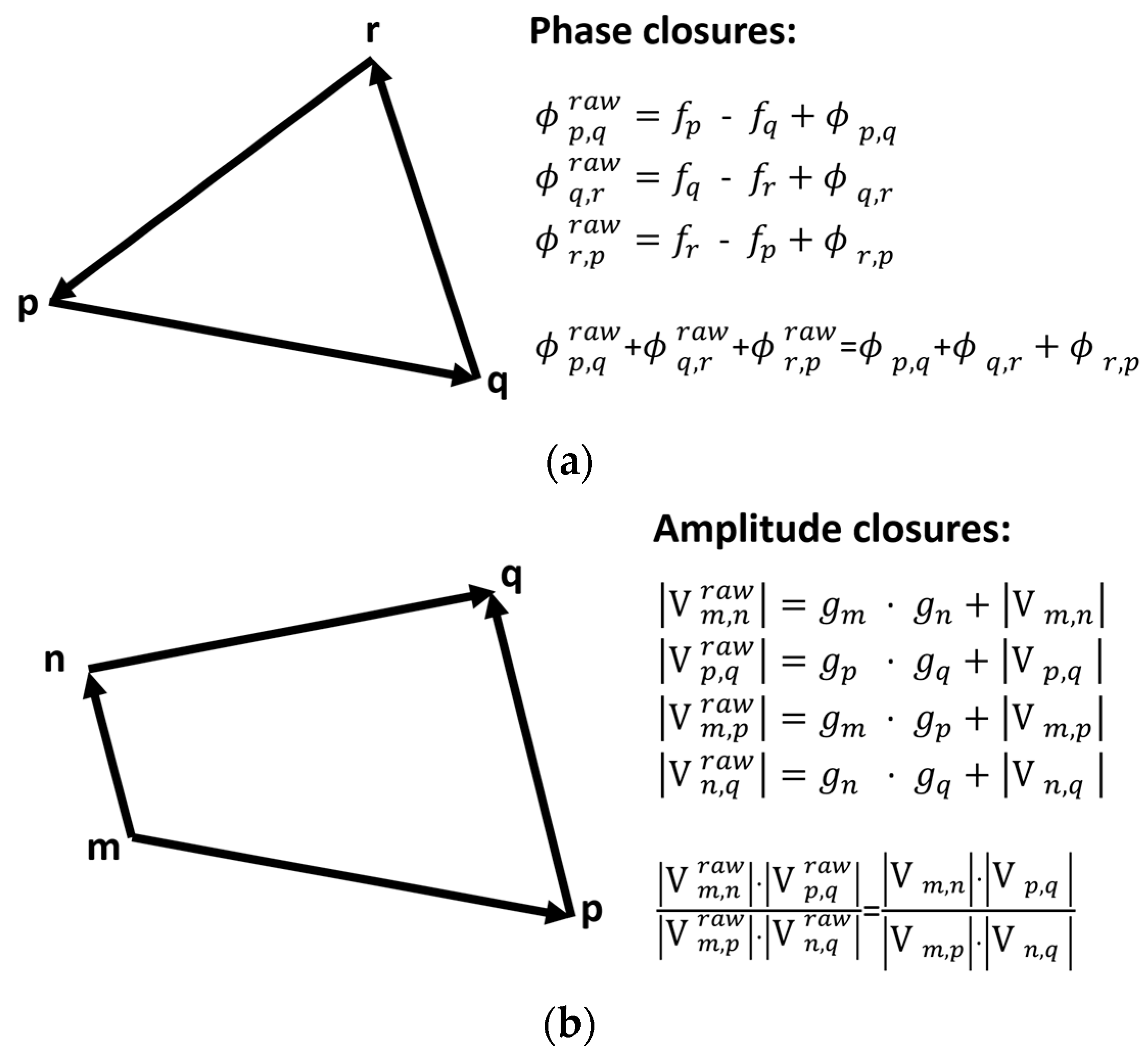
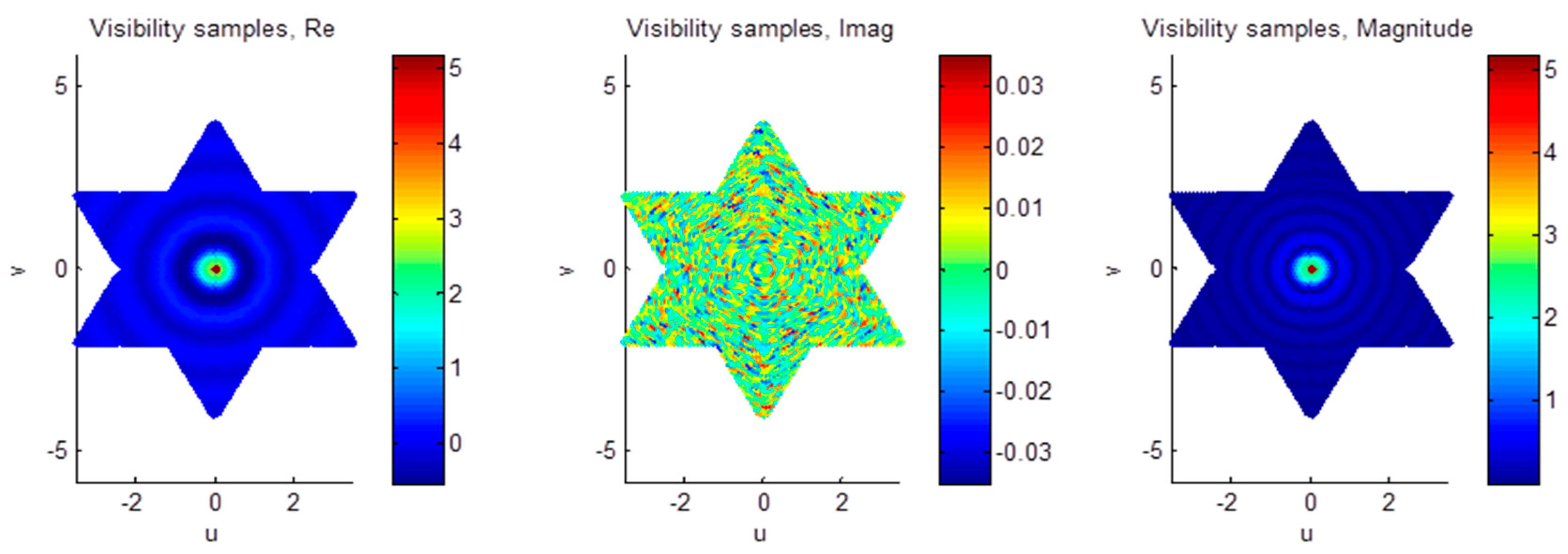
The cross-polarizations VH, HV (or YX, XY) are available only if input BT Maps include non-zero T3 and T4. Using the previous computed data—FWF, antenna patterns, receivers’ physical temperatures and the input BT map—the real and imaginary parts of the visibility samples are simulated through the following expression:

$${\mathrm{V}}_{\mathrm{r}mn}^{pq}\left(\mathrm{u},\mathrm{v},\mathrm{w}\right)=\text{Re}\left[\frac{1}{\sqrt{{\mathsf{\Omega }}_m{\mathsf{\Omega }}_n}}\underset{{\mathsf{\xi }}^2+{\mathsf{\eta }}^2\le 1}{{\displaystyle \iint }}\frac{{\mathrm{T}}_{\mathrm{B}}\left(\mathsf{\xi },\mathsf{\eta }\right)-{\mathrm{T}}_{\text{REC}}}{\sqrt{1-{\mathsf{\xi }}^2-{\mathsf{\eta }}^2}}{\mathrm{F}}_{\mathrm{n},m}\left(\mathsf{\xi },\mathsf{\eta }\right){\mathrm{F}}_{\mathrm{n},n}^{*}\left(\mathsf{\xi },\mathsf{\eta }\right){\tilde{\text{r}}}_{m\mathrm{n}}^{\text{ii}}\left(\Delta \text{t}\right){\mathrm{e}}^{\text{jk}\Delta \mathrm{r}}\mathrm{d}\mathsf{\xi }\mathrm{d}\mathsf{\eta }\right]$$

(2a)

$${\mathrm{V}}_{\mathrm{i}mn}^{pq}\left(\mathrm{u},\mathrm{v},\mathrm{w}\right)=\text{Im}\left[\frac{1}{\sqrt{{\mathsf{\Omega }}_m{\mathsf{\Omega }}_n}}\underset{{\mathsf{\xi }}^2+{\mathsf{\eta }}^2\le 1}{{\displaystyle \iint }}\frac{{\mathrm{T}}_{\mathrm{B}}\left(\mathsf{\xi },\mathsf{\eta }\right)-{\mathrm{T}}_{\text{REC}}}{\sqrt{1-{\mathsf{\xi }}^2-{\mathsf{\eta }}^2}}{\mathrm{F}}_{\mathrm{n},m}\left(\mathsf{\xi },\mathsf{\eta }\right){\mathrm{F}}_{\mathrm{n},n}^{*}\left(\mathsf{\xi },\mathsf{\eta }\right){\tilde{\text{r}}}_{mn}^{\text{qi}}\left(\Delta \text{t}\right){\mathrm{e}}^{\text{jk}\Delta \mathrm{r}}\mathrm{d}\mathsf{\xi }\mathrm{d}\mathsf{\eta }\right]$$

(2b)

where $\Delta \text{r}=-{\mathsf{\lambda }}_0\left(\text{u}\mathsf{\xi }+\text{v}\mathsf{\eta }+\mathrm{w}\sqrt{1-{\mathsf{\xi }}^2-{\mathsf{\eta }}^2}\right)$, the antenna spacing normalized to the electromagnetic wavelength ${\mathsf{\lambda }}_0$ is called the “baseline” $\left(\mathrm{u},\mathrm{v},\mathrm{w}\right)=\left(x_n-x_m,y_n-y_m,z_n-z_m\right)/{\mathsf{\lambda }}_0$, although usually the array elements lie in a plane (w = 0), $\Delta \text{t}=\Delta \text{r}/\mathrm{c}$, the director cosines with respect to the X and Y axes are $\mathsf{\xi }=\sin \left(\vartheta \right)·\cos \left(\phi \right)$ and $\mathsf{\eta }=\sin \left(\vartheta \right)·\sin \left(\phi \right)$, respectively, T_B is the brightness temperature, T_REC is the physical temperature of the receivers, F_n1,2 are the normalized antenna voltage patterns at a given polarization, ${\tilde{\text{r}}}_{mn}^{\text{ii}}$, ${\tilde{\text{r}}}_{mn}^{\text{qi}}$ are the fringe-washing functions (real and imaginary parts), and Ω_m,n are the antenna solid angles [1].

The extension of Equation (2) to the polarimetric case including the cross-polar terms was derived in [2]:

$$\left(T_{B,xx}\left(\mathsf{\xi },\mathsf{\eta }\right)-T_{REC}\right)F_{n,xm}\left(\mathsf{\xi },\mathsf{\eta }\right)F_{n,xn}^{*}\left(\mathsf{\xi },\mathsf{\eta }\right)\to \left(T_{B,xx}\left(\mathsf{\xi },\mathsf{\eta }\right)-T_{REC}\right)R_{n,xm}\left(\mathsf{\xi },\mathsf{\eta }\right)R_{n,xn}^{*}\left(\mathsf{\xi },\mathsf{\eta }\right)+T_{B,yx}\left(\mathsf{\xi },\mathsf{\eta }\right)\left(R_{n,xm}\left(\mathsf{\xi },\mathsf{\eta }\right)C_{n,xn}^{*}\left(\mathsf{\xi },\mathsf{\eta }\right)+C_{n,xm}\left(\mathsf{\xi },\mathsf{\eta }\right)R_{n,xn}^{*}\left(\mathsf{\xi },\mathsf{\eta }\right)\right)+\left(T_{B,yy}\left(\mathsf{\xi },\mathsf{\eta }\right)-T_{REC}\right)C_{n,xm}\left(\mathsf{\xi },\mathsf{\eta }\right)C_{n,xn}^{*}\left(\mathsf{\xi },\mathsf{\eta }\right)$$

(3a)

$$\left(T_{B,yy}\left(\mathsf{\xi },\mathsf{\eta }\right)-T_{REC}\right)F_{n,ym}\left(\mathsf{\xi },\mathsf{\eta }\right)F_{n,yn}^{*}\left(\mathsf{\xi },\mathsf{\eta }\right)\to \left(T_{B,xx}\left(\mathsf{\xi },\mathsf{\eta }\right)-T_{REC}\right)C_{n,ym}\left(\mathsf{\xi },\mathsf{\eta }\right)C_{n,yn}^{*}\left(\mathsf{\xi },\mathsf{\eta }\right)+T_{B,yx}\left(\mathsf{\xi },\mathsf{\eta }\right)\left(R_{n,ym}\left(\mathsf{\xi },\mathsf{\eta }\right)C_{n,yn}^{*}\left(\mathsf{\xi },\mathsf{\eta }\right)+C_{n,ym}\left(\mathsf{\xi },\mathsf{\eta }\right)R_{n,yn}^{*}\left(\mathsf{\xi },\mathsf{\eta }\right)\right)+\left(T_{B,yy}\left(\mathsf{\xi },\mathsf{\eta }\right)-T_{REC}\right)R_{n,ym}\left(\mathsf{\xi },\mathsf{\eta }\right)R_{n,yn}^{*}\left(\mathsf{\xi },\mathsf{\eta }\right)$$

(3b)

$$T_{B,yx}\left(\mathsf{\xi },\mathsf{\eta }\right)F_{n,ym}\left(\mathsf{\xi },\mathsf{\eta }\right)F_{n,xn}^{*}\left(\mathsf{\xi },\mathsf{\eta }\right)\to \left(T_{B,xx}\left(\mathsf{\xi },\mathsf{\eta }\right)-T_{REC}\right)C_{n,ym}\left(\mathsf{\xi },\mathsf{\eta }\right)R_{n,xn}^{*}\left(\mathsf{\xi },\mathsf{\eta }\right)+T_{B,yx}\left(\mathsf{\xi },\mathsf{\eta }\right)\left(R_{n,ym}\left(\mathsf{\xi },\mathsf{\eta }\right)R_{n,xn}^{*}\left(\mathsf{\xi },\mathsf{\eta }\right)+C_{n,ym}\left(\mathsf{\xi },\mathsf{\eta }\right)C_{n,xn}^{*}\left(\mathsf{\xi },\mathsf{\eta }\right)\right)+\left(T_{B,yy}\left(\mathsf{\xi },\mathsf{\eta }\right)-T_{REC}\right)R_{n,ym}\left(\mathsf{\xi },\mathsf{\eta }\right)C_{n,xn}^{*}\left(\mathsf{\xi },\mathsf{\eta }\right)$$

(3c)

$$T_{B,xy}\left(\mathsf{\xi },\mathsf{\eta }\right)F_{n,xm}\left(\mathsf{\xi },\mathsf{\eta }\right)F_{n,yn}^{*}\left(\mathsf{\xi },\mathsf{\eta }\right)\to \left(T_{B,xx}\left(\mathsf{\xi },\mathsf{\eta }\right)-T_{REC}\right)R_{n,ym}\left(\mathsf{\xi },\mathsf{\eta }\right)C_{n,xn}^{*}\left(\mathsf{\xi },\mathsf{\eta }\right)+T_{B,yx}\left(\mathsf{\xi },\mathsf{\eta }\right)\left(C_{n,ym}\left(\mathsf{\xi },\mathsf{\eta }\right)C_{n,xn}^{*}\left(\mathsf{\xi },\mathsf{\eta }\right)+R_{n,ym}\left(\mathsf{\xi },\mathsf{\eta }\right)R_{n,xn}^{*}\left(\mathsf{\xi },\mathsf{\eta }\right)\right)+\left(T_{B,yy}\left(\mathsf{\xi },\mathsf{\eta }\right)-T_{REC}\right)C_{n,ym}\left(\mathsf{\xi },\mathsf{\eta }\right)R_{n,xn}^{*}\left(\mathsf{\xi },\mathsf{\eta }\right)$$

(3d)

where $R_{n,x/ym}\left(\mathsf{\xi },\mathsf{\eta }\right)$ and $C_{n,x/ym}\left(\mathsf{\xi },\mathsf{\eta }\right)$ are, respectively, the normalized co- and cross-polar radiation patterns of antenna m at X or Y polarizations. In the noise injection calibration mode, since the noise is injected by switching the antennas to the outputs of the noise distribution network with S-parameters, the following expression has to be used to simulate the visibility samples:

$${\mathrm{V}}_{mn}^{\text{pq}}\left(\mathrm{u},\mathrm{v},\mathrm{w}\right)={\mathrm{T}}_{\text{NI}}·{\text{FWF}}_0·{\mathrm{S}}_{\text{NI }m,0}{\mathrm{S}}_{\text{NI }n,0}^{*}+\text{ CN}$$

(4)

with ${\mathrm{S}}_{\text{NI }m/n,0}$ the S-parameters of the Noise Injection network from input port 0 to output ports m or n, and with FWF₀ the complex fringe-wash function at the origin, $\text{CN}={\text{T}}_0·\left(\mathrm{I}-{\text{S}}_{\text{NI}}·{\mathrm{S}}_{\text{NI}}^{*}\right)·{\mathsf{\delta }}_{\text{pq}}$, and T₀ = 290 K.

The procedure to compute Equations (1)–(3) is sketched in Figure 2. In the next sections, each submodule is described.

2.1.1. Antenna Array Component

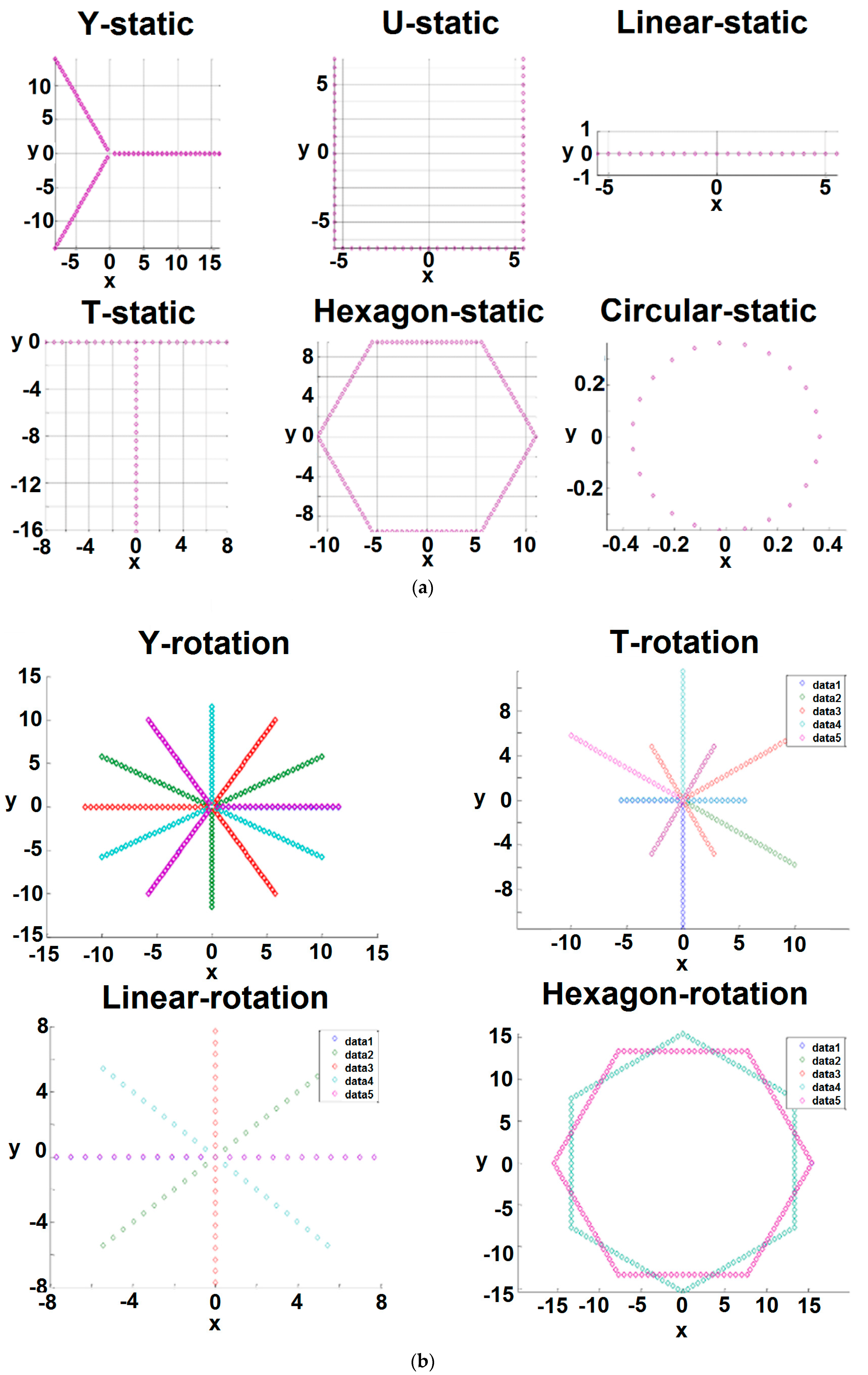
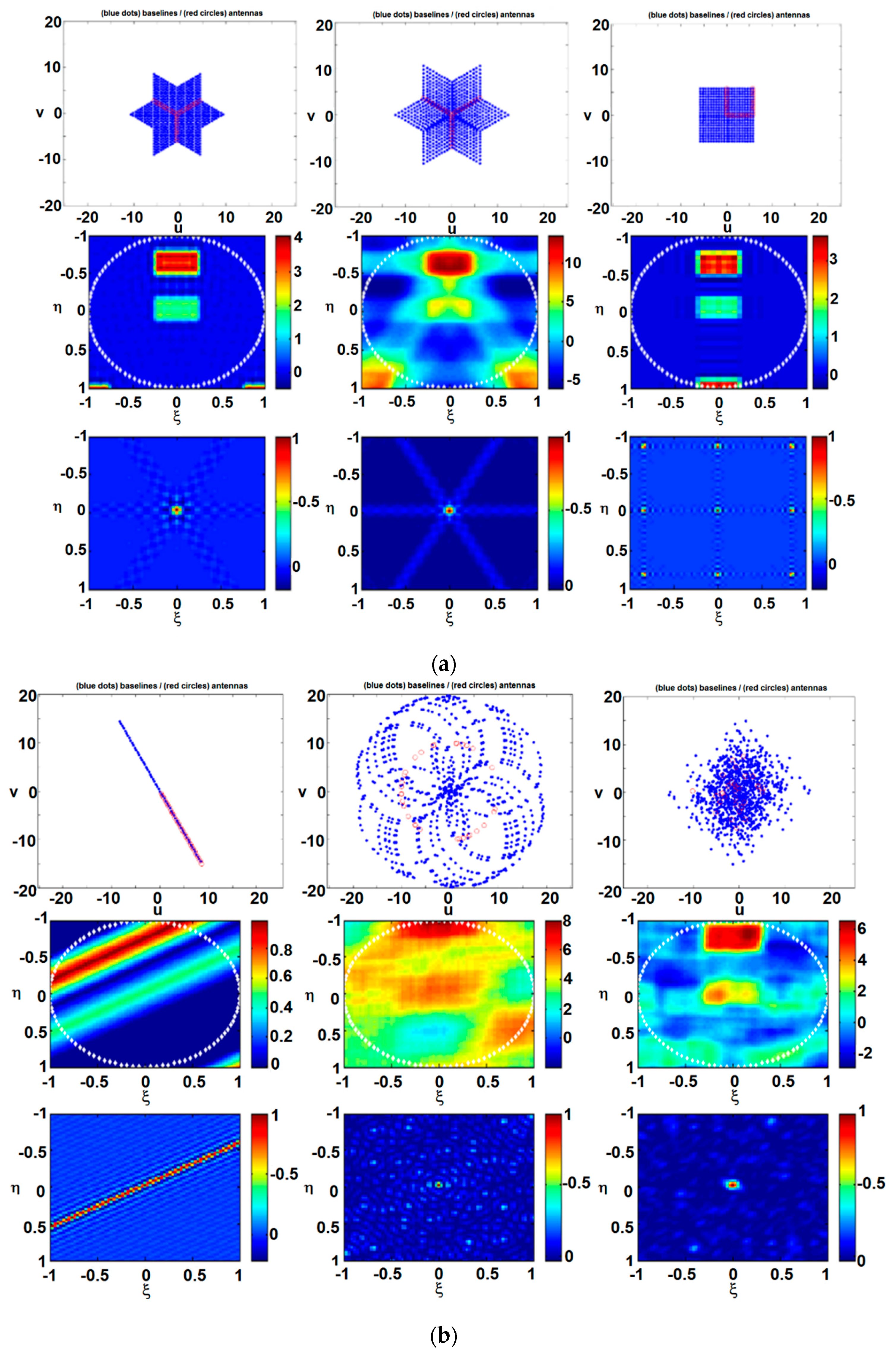
The antenna array is defined by its antenna positions as a function of time including a static array with arbitrary shape, e.g., linear, Y-shaped, T-shaped, random distribution, etc., a static array plus small deviations of the antenna positions as a function of time (e.g., thermal and mechanical oscillations), or an array with arbitrarily moving antennas, e.g., a rotating array. Antenna orientations (i.e., polarizations) can also be static or a function of time.

To make the simulator as generic as possible, the antenna positions $\left(x_n\left(t\right),y_n\left(t\right),z_n\left(t\right)\right)$ and polarization ${\mathsf{\theta }}_n\left(t\right)$ (within the X-Y plane) can be described in the instrument reference frame by mathematical functions as a function of the time:

$$[{\overrightarrow{R}}_n\left(t\right),\mathsf{\theta }\left(t\right)]=\left(x_n\left(t\right),y_n\left(t\right),z_n\left(t\right),{\mathsf{\theta }}_n\left(t\right)\right)$$

(5)

or they can be described in a tabular form to be read from an input file, from which positions at intermediate times are linearly interpolated from the values given in the tables. The angle ${\mathsf{\theta }}_n\left(t\right)$ is defined as the rotation angle of the nth antenna polarization frame with respect to the instrument reference frame.

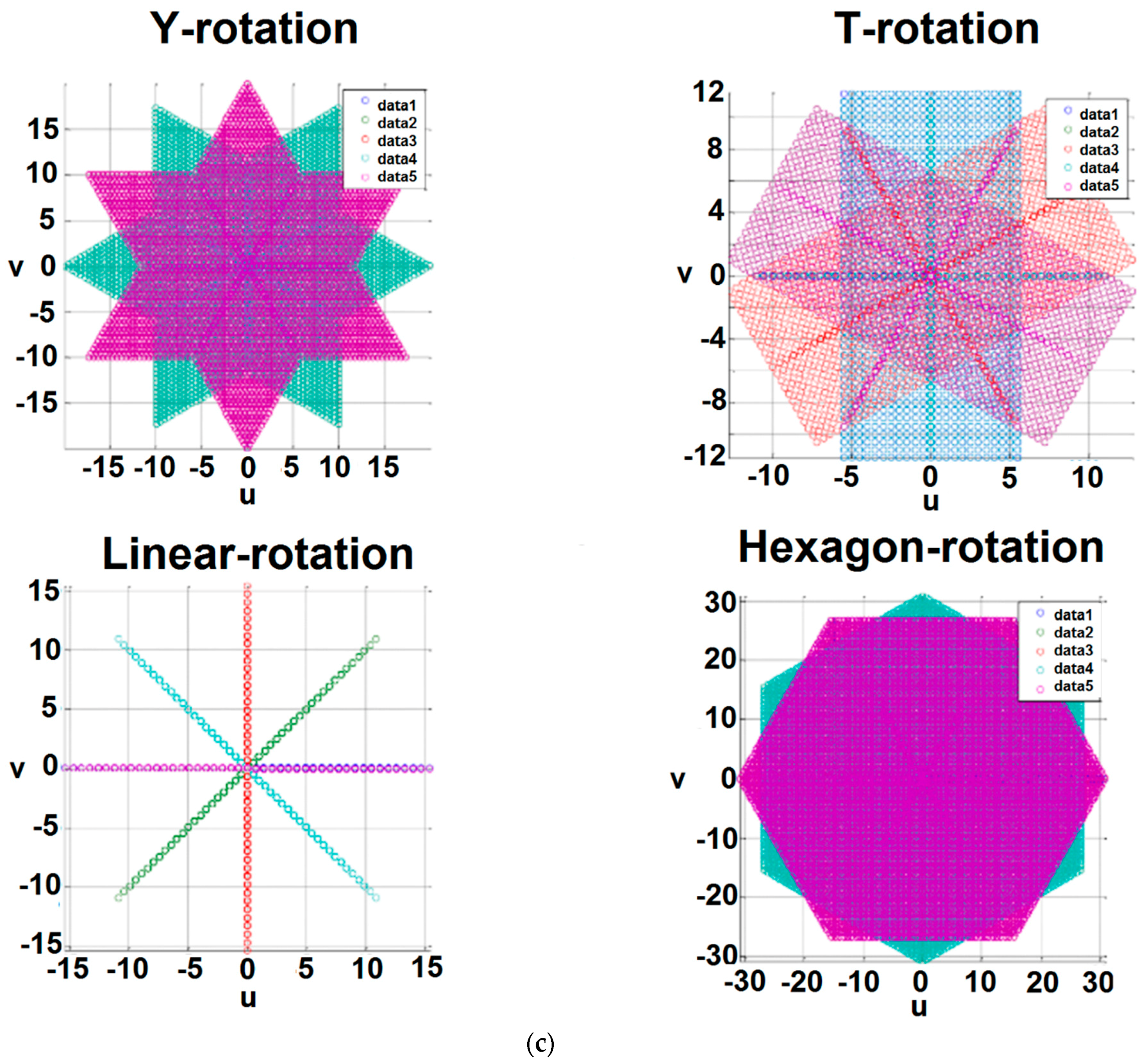
From these parameters, the actual baselines (u_mn, v_mn, w_mn) being measured at each particular time (antenna positions may be moving) are determined. Figure 3 shows sample SAIRPS antenna arrays: (a) static arrays; (b) rotating arrays; and (c) (u, v) points (baselines) measured by the rotating arrays.

In order to be able to process the visibility samples, they need to be changed first from the instrument polarization reference frame to visibilities as correlations between the antennas in their own defined polarization frames:

$$\left[\begin{array}{c}\begin{array}{c}{\mathrm{V}}_{{\mathrm{p}}_m{\mathrm{p}}_n}\\ {\mathrm{V}}_{{\mathrm{p}}_m{\mathrm{q}}_n}\end{array}\\ \begin{array}{c}{\mathrm{V}}_{{\mathrm{q}}_m{\mathrm{p}}_n}\\ {\mathrm{V}}_{{\mathrm{q}}_m{\mathrm{q}}_n}\end{array}\end{array}\right]=\left[\begin{array}{cc}\begin{array}{cc}\text{AC}& -\text{AD}\\ \text{AD}& \text{AC}\end{array}& \begin{array}{cc}-\text{BC}& \text{BD}\\ -\text{BD}& -\text{BC}\end{array}\\ \begin{array}{cc}\text{BC}& -\text{BD}\\ \text{BD}& \text{BC}\end{array}& \begin{array}{cc}\text{AC}& -\text{AD}\\ \text{AD}& \text{AC}\end{array}\end{array}\right]·\left[\begin{array}{c}\begin{array}{c}{\mathrm{V}}_{\text{xx}}\\ {\mathrm{V}}_{\text{xy}}\end{array}\\ \begin{array}{c}{\mathrm{V}}_{\text{yx}}\\ {\mathrm{V}}_{\text{yy}}\end{array}\end{array}\right]$$

(6)

where the elements $A=cos\left({\mathsf{\theta }}_m\left(t\right)\right)$, $B=-sin\left({\mathsf{\theta }}_m\left(t\right)\right)$, and $C=cos\left({\mathsf{\theta }}_n\left(t\right)\right)$, $D=-sin\left({\mathsf{\theta }}_n\left(t\right)\right)$ are the elements of the rotation matrices $\stackrel{=}{\mathrm{R}}\left({\mathsf{\theta }}_m\left(t\right)\right)\text{ and }\stackrel{=}{\mathrm{R}}\left({\mathsf{\theta }}_n\left(t\right)\right)$ defined as $\stackrel{=}{\mathrm{R}}\left({\mathsf{\theta }}_m\left(t\right)\right)=\left[\begin{array}{cc}\mathrm{A}& -\mathrm{B}\\ \mathrm{B}& \mathrm{A}\end{array}\right]\text{ and }\stackrel{=}{\mathrm{R}}\left({\mathsf{\theta }}_n\left(t\right)\right)=\left[\begin{array}{cc}\mathrm{C}& -\mathrm{D}\\ \mathrm{D}& \mathrm{C}\end{array}\right]$.

If the instrument is in dual-polarization only (i.e., ${\mathrm{V}}_{\text{xy}}$ and ${\mathrm{V}}_{\text{yx}}$ are not measured), inverting Equation (6) is not always possible, even assuming ${\mathrm{V}}_{\text{xy}}={\mathrm{V}}_{\text{yx}}=0$, since singularities appear when ${\mathsf{\theta }}_i\left(t\right)={\mathsf{\theta }}_i\left(t\right)=45°$:

$$\left[\begin{array}{c}{\mathrm{V}}_{{\mathrm{p}}_m{\mathrm{p}}_n}\\ {\mathrm{V}}_{{\mathrm{q}}_m{\mathrm{q}}_n}\end{array}\right]=\left[\begin{array}{cc}\text{AC}& \text{BD}\\ \text{BD}& \text{AC}\end{array}\right]·\left[\begin{array}{c}{\mathrm{V}}_{\text{xx}}\\ {\mathrm{V}}_{\text{yy}}\end{array}\right]$$

(7)

Antenna phase center position uncertainties (Δx_n, Δy_n, Δz_n) with respect to the antenna nominal positions (x_n(t), y_n(t), z_n(t)) also account for (x_n(t), y_n(t), z_n(t)) + (Δx_n, Δy_n, Δz_n) in the “direct problem”, meaning the computation of the instrument’s observables, while the estimated (measured on the ground or known from models) antenna phase centers (x_n(t), y_n(t), z_n(t)) are used in the “inverse problem” or image reconstruction from the instrument’s observables.

Antenna patterns (X, Y polarizations, cross-polar terms) appear in Equations (2) and (3) as the F_{n m,n} term. However, these equations implicitly assume that the antennas only pick up radiation from the half hemisphere around the antenna boresight. This is not the case in practice, and both the front and back lobes must be accounted for. The brightness temperature contribution coming from the platform(s) supporting the antennas has been neglected. Other contributions to the brightness temperature coming from the back of the antenna are computed by running the Radiative Transfer Module (companion paper, Part I), but looking in the opposite direction. The equations, including the back lobes, turn out to be exactly the same as Equation (2), but changing “w” to “−w” in the baseline definition, $\Delta r=-{\mathsf{\lambda }}_0\left(\text{u}\mathsf{\xi }+\text{v}\mathsf{\eta }-\mathrm{w}\sqrt{1-{\mathsf{\xi }}^2-{\mathsf{\eta }}^2}\right)$, and, obviously, using the BT distribution present in the back side of the array. The real and imaginary parts of the visibility samples computed from the back lobes (90° < θ ≤ 180°) must be added to the ones computed from the fore lobe (0° ≤ θ ≤ 90°).

$$V_r^{back}\left(u,v\right)=Re\left[\frac{1}{\sqrt{{\mathsf{\Omega }}_m{\mathsf{\Omega }}_n}}\underset{{\mathsf{\xi }}^2+{\mathsf{\eta }}^2\le 1}{{\displaystyle \iint }}\frac{T_B\left(\mathsf{\xi },\mathsf{\eta }\right)-T_{REC}}{\sqrt{1-{\mathsf{\xi }}^2-{\mathsf{\eta }}^2}}{F}_{n,m}^{back}\left(\mathsf{\xi },\mathsf{\eta }\right)F_{n,n}^{back*}\left(\mathsf{\xi },\mathsf{\eta }\right){\tilde{r}}_{mn}^{ii}\left(\Delta t\right)e^{jk\Delta r}d\mathsf{\xi }d\mathsf{\eta }\right]$$

(8a)

$$V_i^{back}\left(u,v\right)=Im\left[\frac{1}{\sqrt{{\mathsf{\Omega }}_m{\mathsf{\Omega }}_n}}\underset{{\mathsf{\xi }}^2+{\mathsf{\eta }}^2\le 1}{{\displaystyle \iint }}\frac{T_B\left(\mathsf{\xi },\mathsf{\eta }\right)-T_{REC}}{\sqrt{1-{\mathsf{\xi }}^2-{\mathsf{\eta }}^2}}{F}_{n,m}^{back}\left(\xi ,\eta \right)F_{n,n}^{back*}\left(\mathsf{\xi },\mathsf{\eta }\right){\tilde{r}}_{mn}^{qi}\left(\Delta t\right)e^{jk\Delta r}d\mathsf{\xi }d\mathsf{\eta }\right]$$

(8b)

Antenna patterns, either ideal, for example ${\left|F_n\left(\mathsf{\theta }\right)\right|}^2=co{s}^n\left(\mathsf{\theta }\right)$ or individually different (from a simulation or a measurement database), co- and cross-polar radiation voltage patterns can be used for the fore (+z) and back (−z) sides of the array. These patterns can also be defined differently for the “direct problem” (computation of the visibility samples from an input brightness temperature map) or the “inverse problem” (image reconstruction from “measured” visibility samples) to allow the estimate of the impact of an imperfect antenna pattern characterization in the radiometric accuracy of the retrieved BT image.

Individual antenna patterns can be either modeled or read from Auxiliary Data Files (ADFs). In SAIRPS the model used consists of an average pattern plus individual random deviations in amplitude and phase over the mean value, and a pointing error described (θ₀, ϕ₀) by two parameters,

$$\begin{array}{c}a=\mathsf{\xi }sin{\mathsf{\theta }}_{0}cos{\mathsf{\varphi }}_0+\mathsf{\eta }sin{\mathsf{\theta }}_{0}sin{\mathsf{\varphi }}_0+\sqrt{1-{\xi }^2-{\eta }^2}cos{\mathsf{\theta }}_0;\hfill \\ b=a^{n/2}\left(1+A_a\cos \left(2\mathsf{\pi }{n}_a\sqrt{1-a^2}+{\Phi }_{\mathrm{a}}\right)\right)e^{j{A}_f\cos \left(2\pi n_f\sqrt{1-a^2}+{\Phi }_{\mathrm{f}}\right)},\hfill \\ \hfill \max \_\mathrm{b}\left(\mathrm{p}\right)=\text{max}\left(\left|b+\mathsf{\epsilon }\right|\right)\hfill \end{array}$$

(9a)

$$\begin{array}{c}{F_n}^{co-polar}\left(i,p,{\left[\xi -\eta \right]}_{unit\_circle}\right)=\frac{b+\epsilon }{\text{max}\left\{b\left(p\right)\right\}},\hfill \\ \hfill {F_n}^{cross-polar}\left(i,p,{\left[\xi -\eta \right]}_{unit\_circle}\right)=\frac{{10}^{CP/20}}{\frac{b+\epsilon }{\text{max}\left\{\mathrm{b}\left(\mathrm{p}\right)\right\}+\epsilon }}\hfill \end{array}$$

(9b)

where n is a parameter used to adjust the antenna beamwidth or, equivalently, the directivity (D = 10log(2(n + 1)), (θ₀, ϕ₀) is the direction of the maximum of the antenna pattern (not necessarily the array boresight +z), A_a and A_f are the magnitudes of the amplitude (with respect to 1) or phase (radians) ripples, n_a and n_f are the frequencies of the amplitude and phase ripples, and Φ_a and Φ_f are the phases of the amplitude and phase ripples to randomize them and avoid all ripples being in phase at the antenna maximum; $\epsilon$ is an arbitrary small number to avoid singularities.

If antenna patterns are read from ADFs (real and imaginary parts), the default angular spacing is set to 1° (i.e., 181 × 361 points in θ and ϕ, one sample/° for both hemispheres); however, if the width of the synthetic beam is narrower, the sampling of the antenna pattern must satisfy the Nyquist criterion, which is at least two samples per angular resolution, or otherwise antenna pattern uncertainties may be underestimated. For example, for a SAIR in a geostationary satellite with a 0.016° angular resolution (10 km), the antenna pattern must be sampled at least every 0.008°.

Once the fore and back sides of the antenna pattern are computed (or read from an ADF), the solid angle is computed by integration of the co- and cross-polar radiation pattern over both hemispheres (4π stereo-radians).

Individual antenna imperfect matching and ohmic losses (η_Ωm = ${\overline{\mathsf{\eta }}}_{\mathsf{\Omega }}$ average plus deviations Δη_Ωm) must also be taken into account to properly compute the overall frequency response and noise figure of each receiving channel. The antenna ohmic losses are modeled as a perfectly matched attenuator of parameters${\left|S_{12}\right|}^2={\left|S_{21}\right|}^2=1/{\eta }_{\mathsf{\Omega }}$, and ${\left|S_{11}\right|}^2={\left|S_{22}\right|}^2=0$, right after an ideal lossless antenna. The antenna physical temperature (T_ph (t)) is also used to compute the actual noise introduced by the antenna ohmic losses, since the noise power at the antenna output is given by a different antenna temperature: $T_A^{\prime }=T_A{\eta }_{\mathsf{\Omega }}+T_{ph}\left(1-{\eta }_{\mathsf{\Omega }}\right)$, and the added noise at the antenna input is given by $\Delta T_R=T_{ph}\left(1/{\eta }_{\mathsf{\Omega }}-1\right)$.

Coupling between different antenna elements produces two effects: a distortion of the antenna pattern itself that appears as ripples with a spatial frequency equal to the baseline between the two antennas being coupled, and a cross-correlation offset coming from the backwards noise radiated by the receiver that is coupled to a neighbor antenna. The second effect will be analyzed in Section 2.1.2. The antenna array coupling is characterized by the S-parameters of a multi-port circuit in which each antenna is a port.

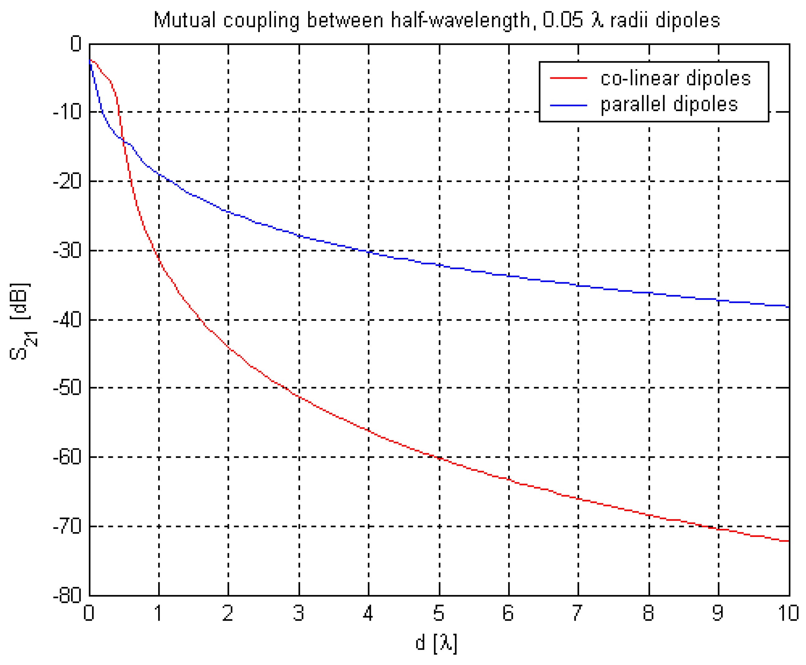
In order to account for the proper distance and orientation dependence of the mutual coupling, the antenna coupling model implemented is based on the coupling between linear dipoles in arbitrary positions and orientations, but scaled by a user-defined factor to simulate the absolute value of the coupling. Figure 4 shows the simulated antenna coupling (S₂₁) between two parallel or collinear half-wavelength dipoles as a function of the distance in terms of the wavelength. As expected, the mutual coupling between collinear dipoles (in red) is much weaker and decreases faster than between the parallel dipoles (in blue). 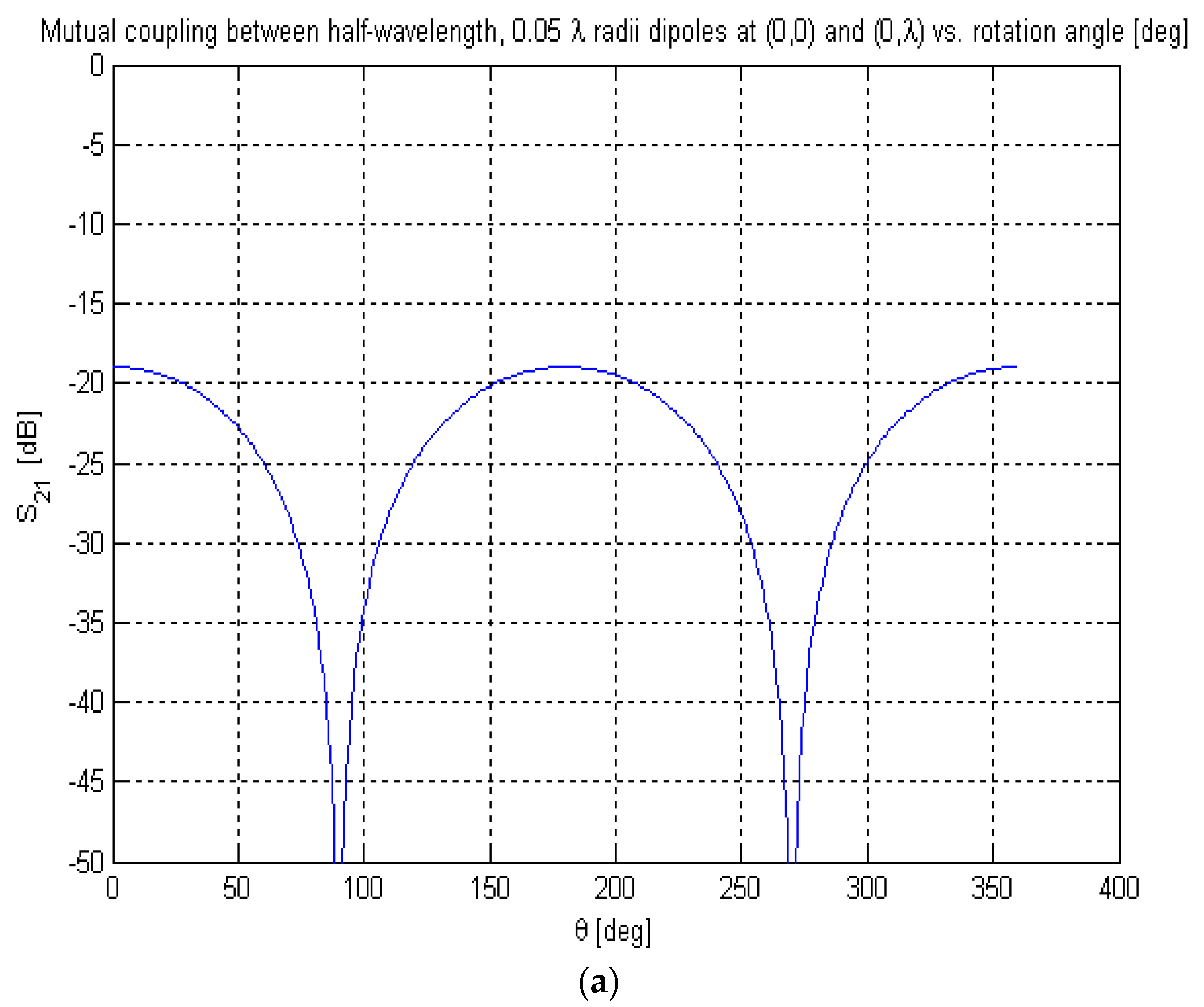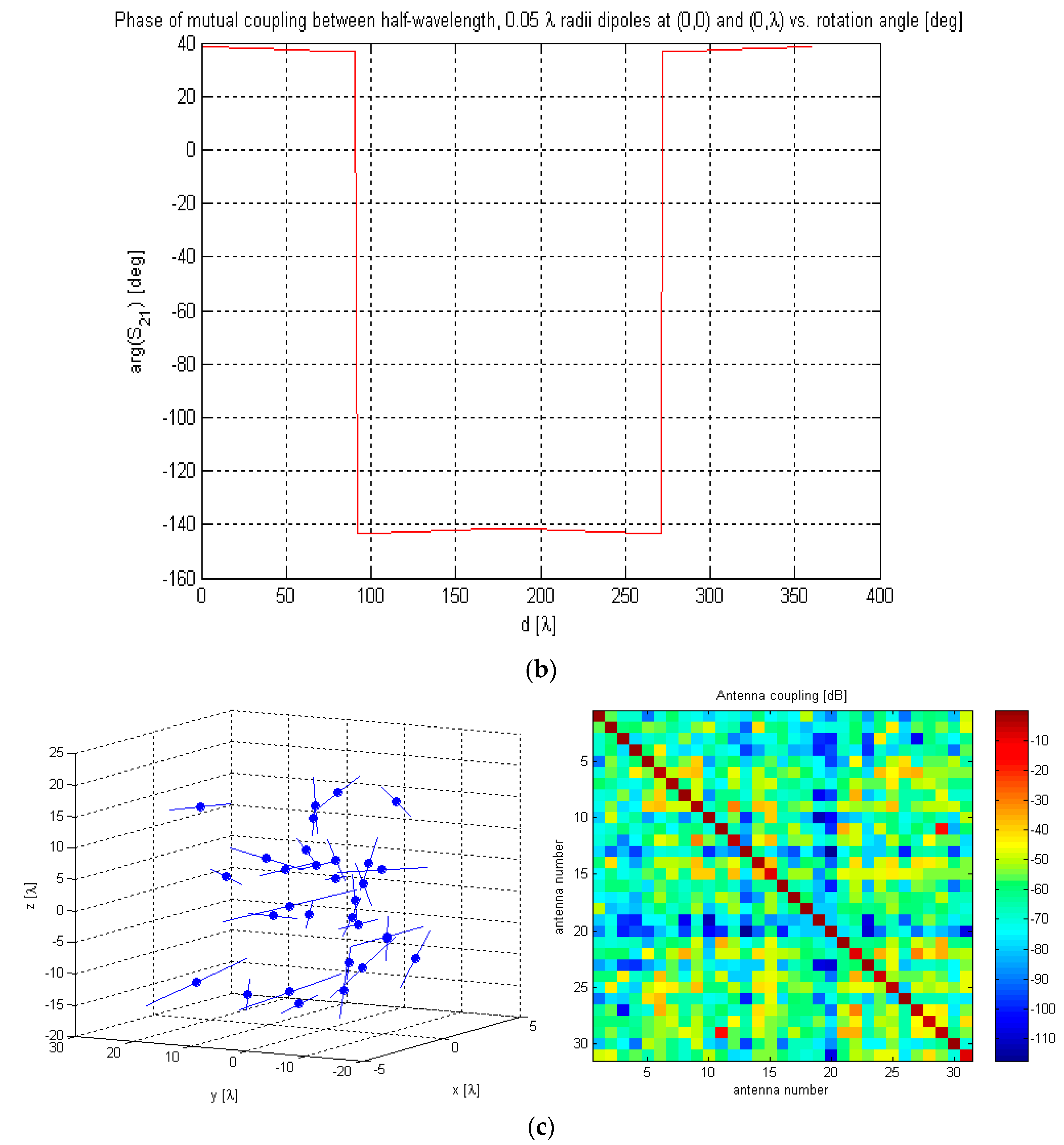Figure 5 shows the simulated antenna coupling (S₂₁) in amplitude and phase between two co-planar half-wavelength dipoles at (0,0) and (0,λ) as a function of the angle between their axes. As expected, coupling is at maximum when they are parallel and at minimum (zero) when they are perpendicular. This model allows us to simulate in a realistic way complex three-dimensional (3D) arrays with arbitrary configurations and antenna orientations such as the one shown in Figure 5c.

The measured visibility samples under antenna coupling conditions can be computed through the mutual coupling matrix $\stackrel{=}{C}$, as defined in [3,4]:

$${\stackrel{=}{V}}^{withcoupling}={\stackrel{=}{C}}^{-1}{\stackrel{=}{V}}^{withoutcoupling}{({\stackrel{=}{C}}^{-1})}^H$$

(10)

where the element V_mn of the visibility matrix $\stackrel{=}{V}$ corresponds to the cross-correlation between the signals collected by antennas m and n, and the $\stackrel{=}{C}$ matrix is defined as:

$$\stackrel{=}{C}=\frac{Z_{in}+Z_L}{Z_L}\left\{\stackrel{=}{I}+\frac{1}{Z_{in}+Z_L}\left[\stackrel{=}{Z}-Z_{in}\stackrel{=}{I}\right]\right\}$$

(11)

where Z_in and Z_L are the input and load impedances of the antennas (assumed all to be the same for the sake of simplicity), and $\stackrel{=}{Z}$ is the Z-parameter matrix and it is given by:

$$\stackrel{=}{Z}=Z_0·{\left(\stackrel{=}{I}-\stackrel{=}{S}\right)}^{-1}·\left(\stackrel{=}{I}+\stackrel{=}{S}\right)$$

(12)

where $\stackrel{=}{I}$ and $\stackrel{=}{S}$ are the identity and the S-parameter matrices, and $Z_0$ is the characteristic impedance.

Equation (10) shows that antenna coupling actually produces a mix of the visibility samples whose main effect is moving energy from the shortest baselines (larger amplitude) to the longest ones (smaller amplitude). This effect can also be understood as a visibility offset given by:

$${\stackrel{=}{V}}^{offset}={\stackrel{=}{V}}^{withcoupling}-{\stackrel{=}{V}}^{withoutcoupling}$$

(13)

An alternative way to interpret Equation (10) is as a linear combination of the isolated antenna patterns with a phase term equal to the baseline and amplitude proportional to the mutual impedance [4]. For a linear array of antennas spaced d wavelengths along the z axis (e.g., at positions 0, d, 2d, 3d…), antenna coupling consists of a modification of the antenna patterns, following the approximate formula below:

$$F_{\mathrm{n},1}^{withcoupling}\approx \frac{Z_L}{Z_L+Z_{in}}\left\{F_{\mathrm{n},1}^{withoutcoupling}-{\displaystyle \sum }_{\forall m\ne 1}\frac{Z_{1\mathrm{m}}}{Z_L+Z_{in}}{F}_{\mathrm{n},\mathrm{m}}^{withoutcoupling}{e}^{jk\left(\mathrm{m}-1\right)·d·sin\theta }\right\}$$

(14)

where $F_{\mathrm{n},\mathrm{m}}^{with/withoutcoupling}$ is the mth normalized antenna voltage pattern with/without the effect of mutual coupling, and Z_1m is the mutual impedance between elements 1 and m, and d is the basic antenna spacing (in wavelengths).

The second term in the brackets in Equation (13) represents the oscillations in the antenna pattern due to the mutual coupling effects.

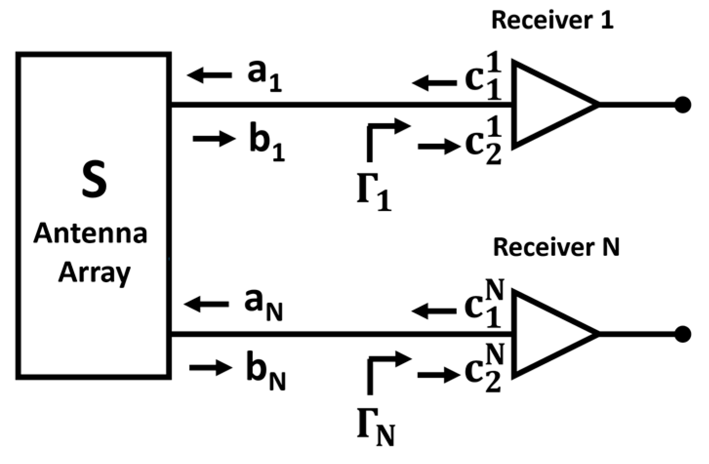
2.1.2. Receiver Component

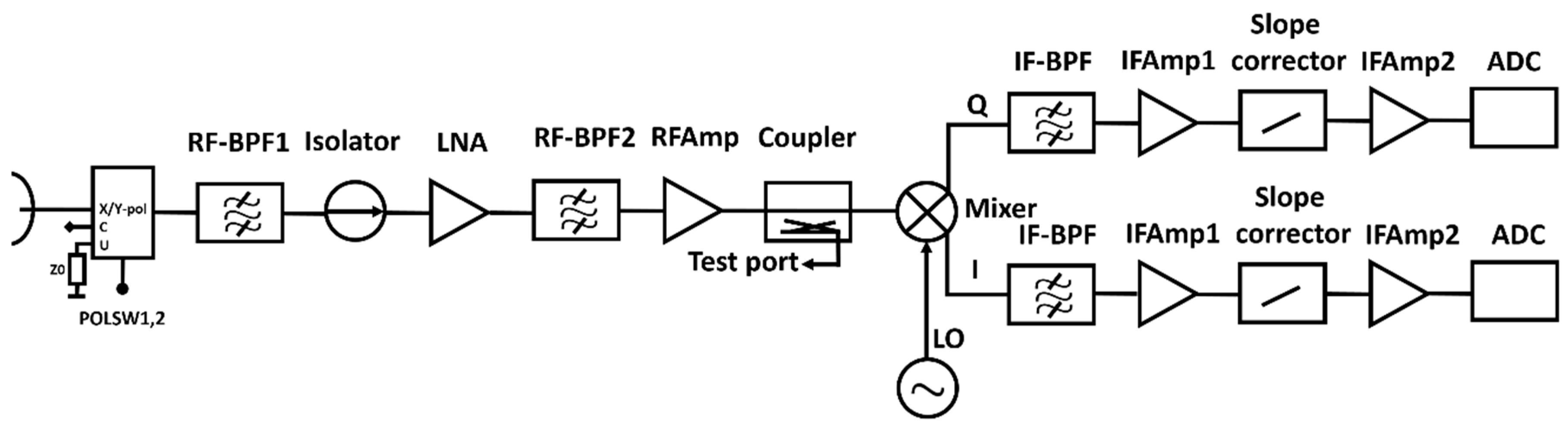
The receiver model is sketched in Figure 6. It is composed of: (1) a switch that selects the input to the receiver channels from the antenna ports (either X or Y polarization, the receiver is duplicated for both polarizations), uncorrelated noise injection at port U (50 Ω matched load), and correlated noise injection at port C; (2) the radio frequency (RF) path composed of a first RF band-pass filter (RF-BPF1), an isolator, an LNA, and a second RF band-pass filter (RF-BPF2), an RF amplifier (RFAmp), and a coupler; (3) an I/Q mixer and local oscillator (LO); and (4) the intermediate frequency (IF) in-phase and quadrature (I/Q) paths, both composed by an IF band-pass filter (IF-BPF), a first IF amplifier (IFAmp1), a slope corrector, a second IF amplifier (IFAmp2), and the analog-to-digital converter (ADC with an arbitrary number of bits, sampling frequency, jitter, etc.). Note that depending on the selected values for the central frequencies, bandwidths, and receiver topology (e.g., lack of an image rejection filter), results may have no sense. The user must be educated in RF engineering and check that the resulting fringe-washing function (Equation (25)) is correct.

In this generic model, receivers’ central frequency and bandwidths for the elements can be arbitrarily defined, as in the most general case, and input data can be read from ADFs with the complex S-parameter matrices as a function of frequency.

Modeling of Receiving Chains Frequency Response

To calculate the fringe-washing functions ${\tilde{r}}_{12}^{ii}\left(\tau \right)$ and ${\tilde{r}}_{12}^{qi}\left(\tau \right)$ for the real and imaginary parts of the visibility function computed between antenna elements 1 and 2, the frequency response of receiving chains must be computed first (different for X and Y polarizations, and for the real and imaginary parts, since after the mixer the in-phase and quadrature branches are separated; see Equation (2a) and (2b)). Regardless of how the frequency response is evaluated, by cascading the S-parameters of each subsystem (noise parameters for the active subsystems are also included) or using end-to-end frequency response ADFs, the long-term gain drifts are included by means of the temperature sensitivity coefficients (nominal temperature = 25°), or as different frequency response ADFs for different temperatures. The correlated noise generated by passive components is evaluated using the S-parameters, and the noise generated by the active subsystems is modeled by the minimum noise figure, the optimum input reflection coefficient, and the equivalent noise "resistance", as a function of frequency, at each physical temperature.

The short-term gain fluctuations (ΔG) due to flicker noise, which limit the ultimate stability that can be achieved, are modeled in a similar way to jitter, and are used in the snapshot, time-evolution, and MonteCarlo simulation modes. The local oscillator is modeled by its central frequency, phase noise and thermal floor noise level, which are converted into a jitter error, and a correlator offset through the mixer finite isolation, respectively. ADCs are modeled by the number of bits, quantization levels uniformly or non-uniformly distributed, and a mathematical transfer function to model saturation, clipping, etc., and skew and jitter errors. The correlator is modeled according to the number of bits, their distribution, and the mathematical transfer function that relates input and output, sampling frequency, jitter, etc.

The failure of a receiver is modeled by forcing a zero in all baselines in which this receiver intervenes, and the failure of a correlator by forcing a zero in only the two baselines computed by that correlator (it and its Hermitian one).

The RF subsystems (amplifiers, filters, isolators, mixer, IF filter and IF attenuator) are typically described by their S-parameters, while the IF sections (filter, amplifiers, etc.) at VHF and UHF are described by the insertion losses (or gain) and voltage standing wave ratio (VSWR). Since, in the pass-band, the VSWR is typically quite small (<1.10), and propagation effects can be neglected, the S-parameters will be:

$$\left|S_{11}\right|=\left|S_{22}\right|=\frac{VSWR-1}{VSWR+1}$$

(15a)

$${\left|S_{21}\right|}^2=\{\begin{array}{c}IL\text{ for filters}\\ G\text{ for amplifiers}\end{array}$$

(15b)

and

$${\left|S_{12}\right|}^2=\{\begin{array}{c}{\left|S_{21}\right|}^2\text{ for filters}\\ 0\text{ for amplifiers}\end{array}$$

(15c)

By transforming the S-parameters into the transmission (ABDC) matrices [5]:

$$A=\frac{\left(1+S_{11}\right)\left(1-S_{22}\right)+S_{12}{S}_{21}}{2S_{21}},B=Z_0\frac{\left(1+S_{11}\right)\left(1+S_{22}\right)-S_{12}{S}_{21}}{2S_{21}}$$

(16a)

$$C=\frac{1}{Z_0}\frac{\left(1-S_{11}\right)\left(1-S_{22}\right)-S_{12}{S}_{21}}{2S_{21}},D=\frac{\left(1-S_{11}\right)\left(1+S_{22}\right)+S_{12}{S}_{21}}{2S_{21}}$$

(16b)

the response of the different subsystems can be easily computed by multiplication of the transmission matrices. Finally, the end-to-end S-parameters are computed as:

$$S_{11}=\frac{A+B/Z_0-C{Z}_0-D}{A+B/Z_0+C{Z}_0+D},S_{21}=\frac{2}{A+B/Z_0+C{Z}_0+D},$$

(17a)

$$S_{12}=\frac{2\left(AD-BC\right)}{A+B/Z_0+C{Z}_0+D},S_{22}=\frac{-A+B/Z_0-C{Z}_0+D}{A+B/Z_0+C{Z}_0+D},$$

(17b)

since subsystems in the receiver block diagram may or may not be present. In case they are not present, their ABCD matrix becomes A = D = 1, B = C = 0 at all frequencies. For the mixer, different gains are considered in both outputs (I and Q), as well as in input and output reflection coefficients and the phase difference between both outputs (quadrature error). This allows us to compute the equivalent S-parameters of the mixer, using the same formulas above, and the different responses of the I and Q branches.

The first two subsystems after the mixer (the IF filter and the IF slope corrector) also use the S-parameter representation since they are based on a 50 Ω reference impedance. The same formulas are used to compute the cascaded S-parameters, but they are shifted to the RF band, in order to get the equivalent overall RF response, and the values for RF frequency values lower than that of the local oscillator are the conjugates of those at their image frequency.

The RF and IF filters are critical because they shape the frequency response to a large extent. They can either be read from a data file, or they can be computed from an analytical model, by default an eighth-order Chebychev band-pass filter, with nominal ripple (e.g., 0.5 dB), user-defined lower and higher band frequencies, user-defined Q-factor of the resonators (e.g., 1000), component tolerance, including inverter constants, and temperature sensitivity of the components. The IF filter is described in a similar way, but in this case it can be a third-order Chebyschev lumped element band-pass filter, with a user-defined Q-factor of the resonators (e.g., 100), component tolerance, and a temperature coefficient of inductors, capacitors and the Q-factor. The S-parameters of each filter are then computed, applying random number generators for each individual parameter, along with the temperature coefficient.

Noise Modeling

The simplest way to compute the receivers’ noise temperature consists of computing the available power gain of each RF subsystem from its S-parameters:

$$G_{av}=\frac{{\left|S_{21}\right|}^2(1-{\left|{\mathsf{\Gamma }}_s\right|}^2)}{{\left|1-{\mathsf{\Gamma }}_s{S}_{11}\right|}^2(1-{\left|{\mathsf{\Gamma }}_0\right|}^2)}$$

(18)

where Γ_s is the corresponding source reflection coefficient, and Γ₀ the output reflection coefficient, computed as:

$${\mathsf{\Gamma }}_0=S_{22}+\frac{S_{12}{S}_{21}{\mathsf{\Gamma }}_s}{1-{\mathsf{\Gamma }}_s{S}_{11}}$$

(19)

For all the passive subsystems, the equivalent noise temperature is given by:

$$T_e=T_{ph}\left(\frac{1}{G_{av}}-1\right)$$

(20)

where T_ph is the physical temperature.

Then, for the active subsystems, LNA, RF and IF amplifiers, the noise temperature is directly read from the instrument database. Finally, the overall noise temperature is computed at each frequency using the Friis formula [5]:

$$T_R=T_1+\frac{T_2}{G_1}+\dots$$

(21)

Note that, because the input switch can have different S-parameters in each of the states, ${\stackrel{=}{S}}_c$, ${\stackrel{=}{S}}_u$, and ${\stackrel{=}{S}}_a$ can be different, and the noise temperatures as seen from the correlated noise input, from the uncorrelated noise input, and from the antenna input can be different as well.

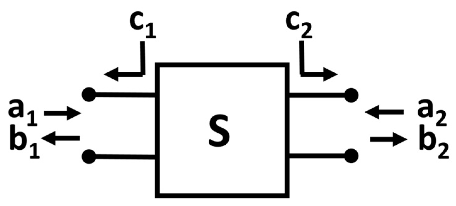
However, the modeling of the noise in an interferometric radiometer has to be much more accurate: backwards noise and the cross-correlation between the forward and backward noise waves are required. A full noise wave analysis is required to evaluate the correlation between outgoing noise waves c₁ and c₂ in two ports, and it is detailed in [6]. These noise waves add to the outgoing signal waves b₁ and b₂ (Figure 7), as follows:

$$\left[\begin{array}{c}{b}_1\\ b_2\end{array}\right]=\left[\begin{array}{cc}{S}_{11}& S_{12}\\ S_{21}& S_{22}\end{array}\right]\left[\begin{array}{c}{a}_1\\ a_2\end{array}\right]+\left[\begin{array}{c}{c}_1\\ c_2\end{array}\right]$$

(22)

The power of the noise waves c₁ and c₂ and their correlation is given by Equations (23a)–(23d) from [6] (except for the Boltzmann’s constant term, omitted below).

$$\overline{{\left|c_1\right|}^2}=T_{min}({\left|S_{11}\right|}^2-1)+t\frac{{\left|1-S_{11}{\mathsf{\Gamma }}_{opt}\right|}^2}{{\left|1+{\mathsf{\Gamma }}_{opt}\right|}^2}$$

(23a)

$$\overline{{\left|c_2\right|}^2}={\left|S_{21}\right|}^2\left(T_{min}+t\frac{{\left|{\mathsf{\Gamma }}_{opt}\right|}^2}{{\left|1+{\mathsf{\Gamma }}_{opt}\right|}^2}\right)$$

(23b)

$$\overline{c_1{c}_2^{*}}=-t\frac{S_{21}^{*}{\mathsf{\Gamma }}_{opt}^{*}}{{\left|1+{\mathsf{\Gamma }}_{opt}\right|}^2}+\frac{S_{11}}{S_{21}}\overline{{\left|c_2\right|}^2}$$

(23c)

and

$$t=\frac{4T_0{R}_n}{Z_0}$$

(23d)

where T₀ = 290 K, Z₀ is the normalization impedance, T_min is the minimum noise temperature that will be attained when the device is charged with Γ_opt at the input, Γ_opt is the input reflection coefficient which provides the best noise performance, and R_n is the equivalent noise "resistance". These four parameters (Γ_opt is complex) are the ones that describe the noise performance of an active device, and they can be mapped into the four noise wave parameters ${\left|c_1\right|}^2$, ${\left|c_2\right|}^2$, and $c_1{c}_2^{*}$ (which is also complex). In order to refer $\overline{{\left|c_2\right|}^2}$ and $\overline{c_1{c}_2^{*}}$ at the input, it suffices to divide Equation (23b) by ${\left|S_{21}\right|}^2$, and Equation (23c) by $S_{21}^{*}$ (see Equation (10) in [6]).

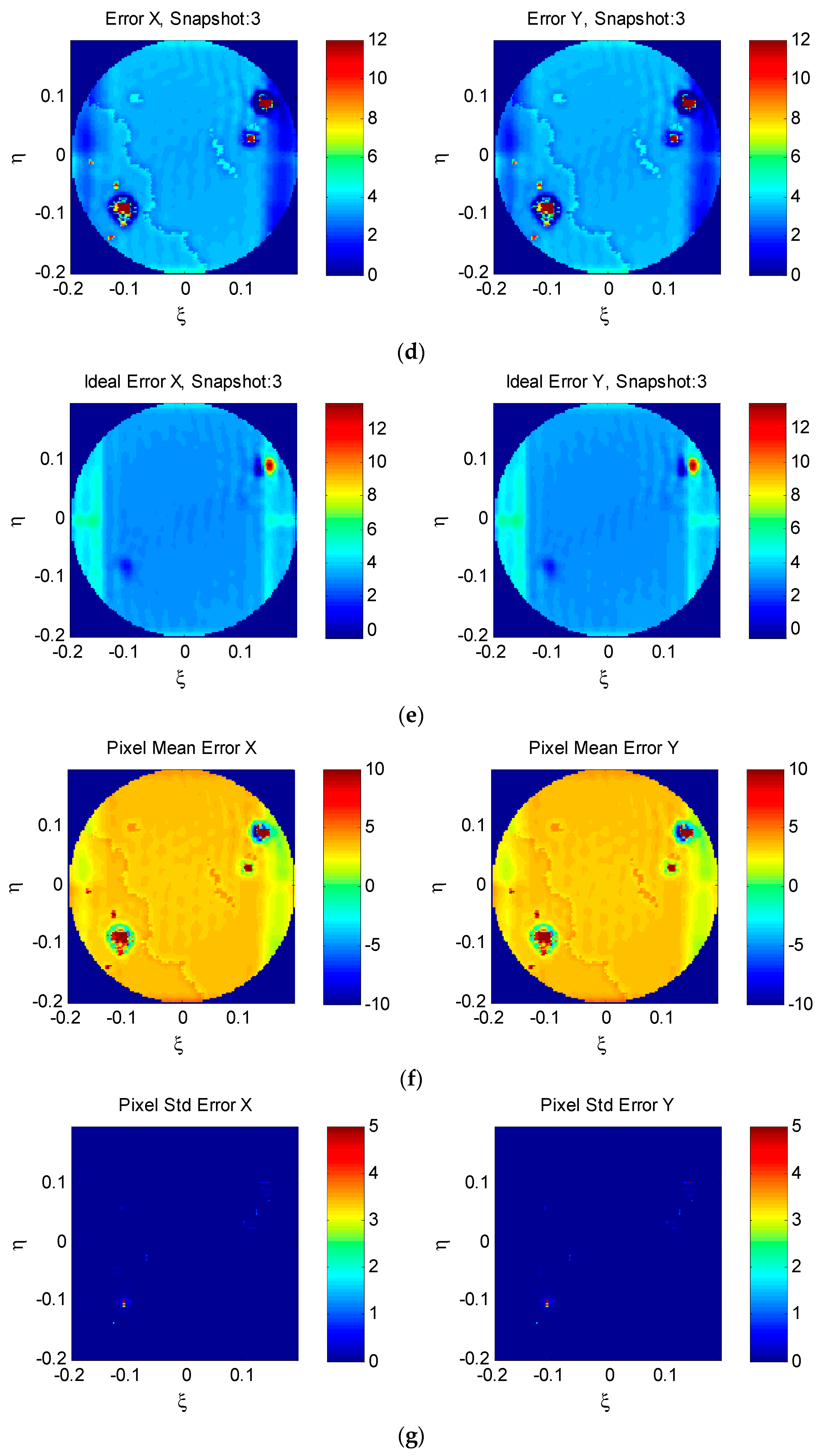
The finite antenna coupling and the cross-correlation between the outgoing noise waves (Equation (23c)) introduces an offset in the visibility samples (Figure 8). All noise waves are referred at the antenna reference frame (after an ideal lossless antenna, but before the attenuator that models the antenna ohmic losses, so that the wave amplitudes do not need to be re-scaled).

All effects, including imperfect matching both at the antenna side and at the receiving chain side can be obtained by:

$${\stackrel{=}{\mathrm{V}}}_{\text{backwards}}=\stackrel{=}{\mathsf{\Lambda }}·\stackrel{=}{\mathrm{S}}·\text{diag}\left(\overline{{\mathrm{T}}_{\mathrm{c}}}\right)+\stackrel{=}{\mathsf{\Lambda }}·\stackrel{=}{\mathrm{S}}·\text{diag}\left(\overline{{\mathrm{T}}_{\mathrm{r}}}\right)·{\stackrel{=}{\mathrm{S}}}^{\mathrm{H}}·{\stackrel{=}{\mathsf{\Lambda }}}^{\mathrm{H}}+\text{diag}\left(\overline{{\mathrm{T}}_{\mathrm{R}}}\right)+\text{diag}\left({\overline{{\mathrm{T}}_{\mathrm{c}}}}^{*}\right)·{\stackrel{=}{\mathrm{S}}}^{\mathrm{H}}·{\stackrel{=}{\mathsf{\Lambda }}}^{\mathrm{H}}$$

(24)

where $\stackrel{=}{\mathrm{S}}$ is either the S-parameter matrix of the antenna array (same as in Equation (12)) or the noise injection S-parameters when the input switch is in noise injection calibration mode, $\stackrel{=}{\mathsf{\Lambda }}$ is a diagonal matrix with the reflection coefficients of each port, diag($\overline{x}$) is an operator that converts the elements of the vector $\overline{x}$ in a diagonal matrix, and $\overline{{\mathrm{T}}_{\mathrm{c}}}$, $\overline{{\mathrm{T}}_{\mathrm{r}}}$, and $\overline{{\mathrm{T}}_{\mathrm{R}}}$ are the equivalent noise temperatures associated with $\overline{{\left|c_1\right|}^2}$, $\overline{{\left|c_2\right|}^2}$, and $\overline{c_1{c}_2^{*}}$. Note that neither the antennas’ nor the receivers’ input need to be perfectly matched and that ${\stackrel{=}{\mathrm{V}}}_{\text{backwards}}$ will be slightly different when the input switch is connected to the antennas or to the noise distribution network.

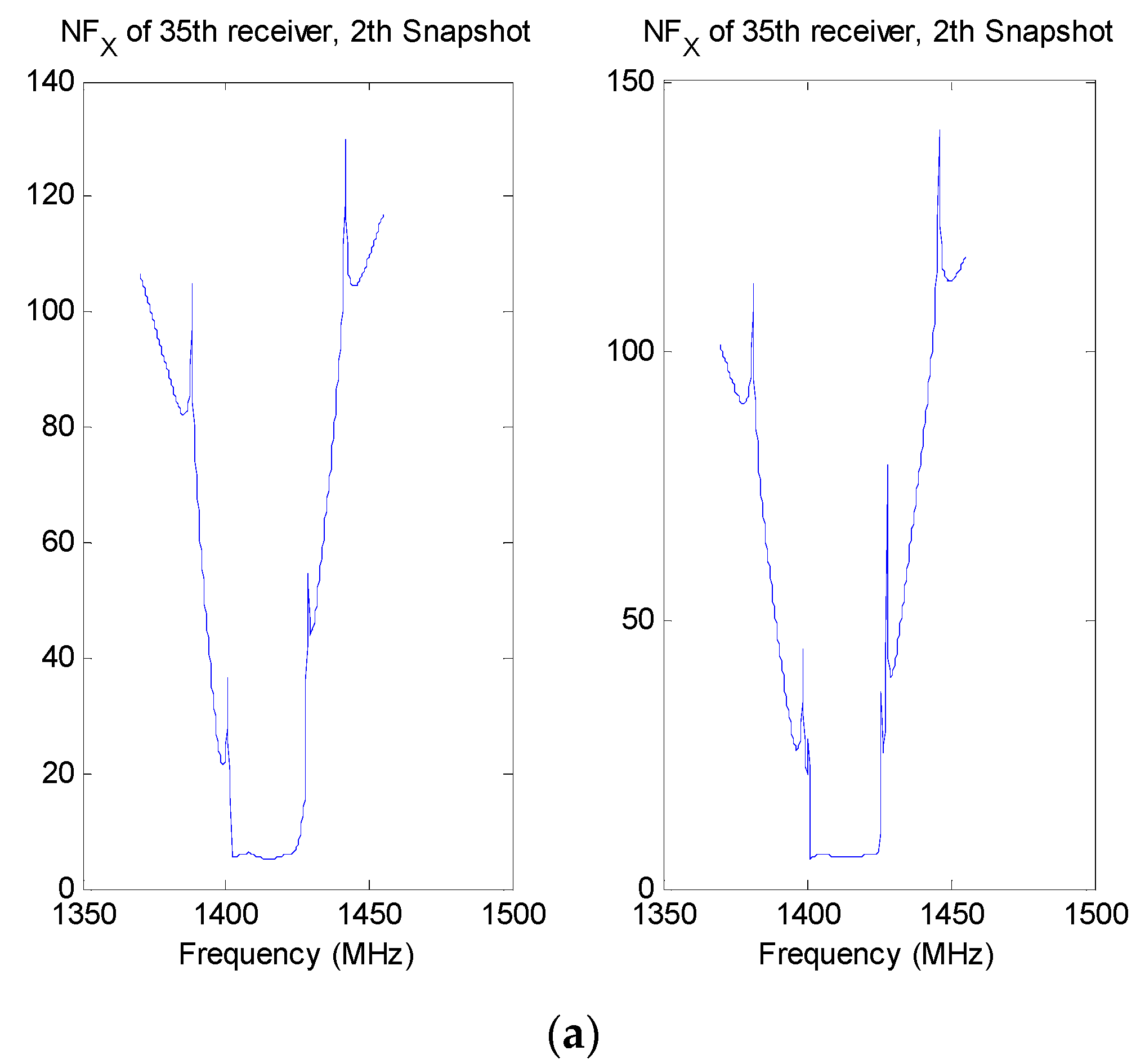
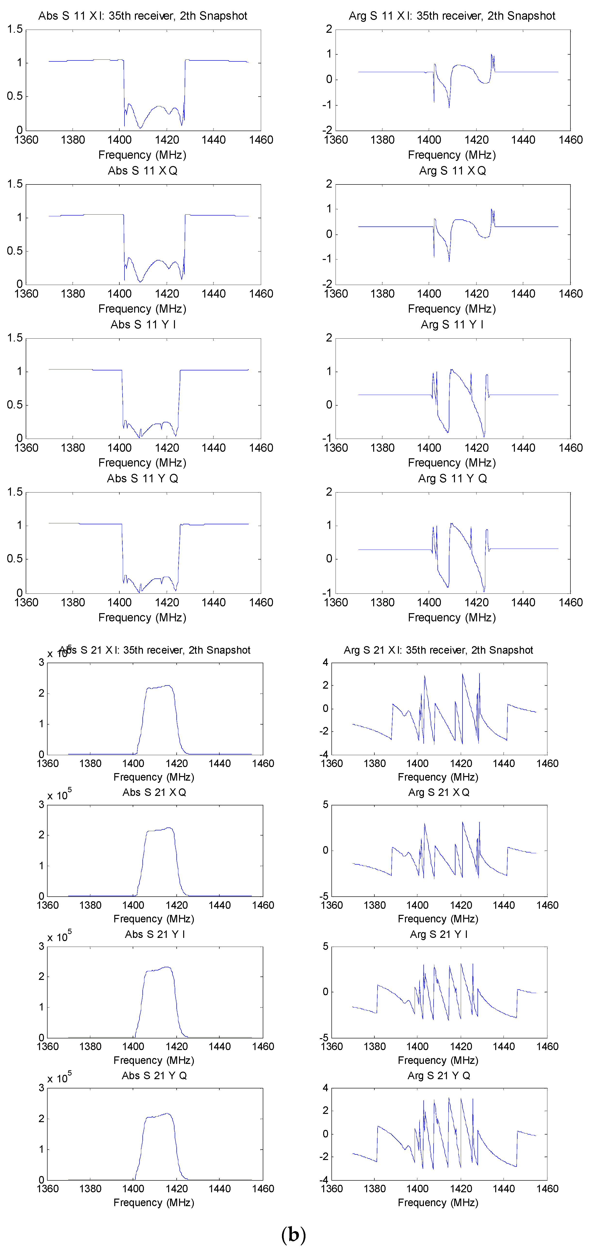
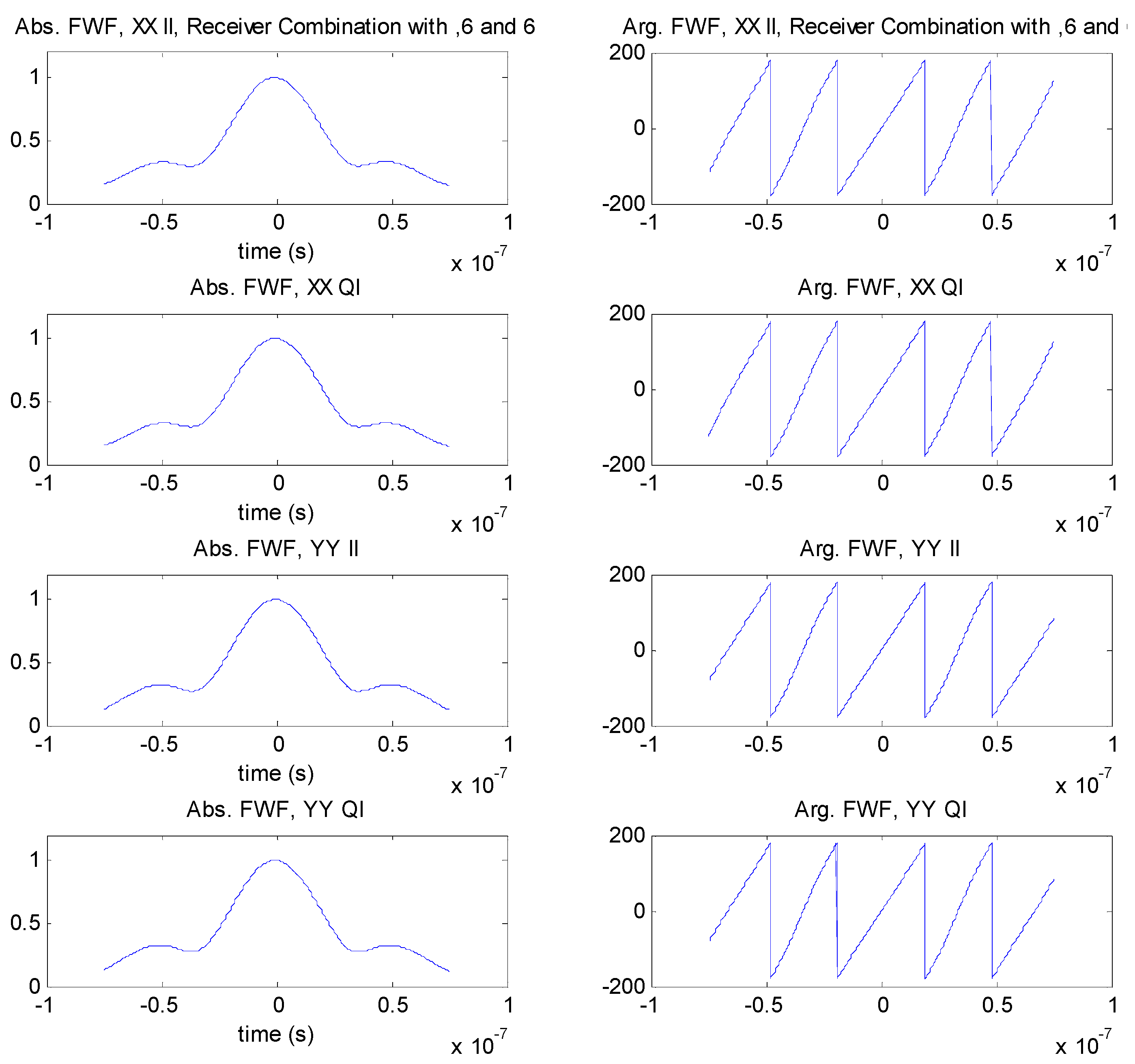
Figure 9 shows an example of the receivers’ modeling of a SMOS-like instrument (Soil Moisture and Ocean Salinity mission) at the L-band: (a) the noise figure as a function of the frequency for the I- and Q-channels; (b) the S₁₁ and S₂₁ parameters (amplitude and phase, X- and Y-polarizations, I- and Q-channels); and (c) the end-to-end frequency responses (amplitude and phase) for X- and Y-polarizations, I- and Q-channels.

Modeling the Fringe Washing Function

Since the I- and the Q-branches may have slightly different frequency responses, the fringe-wash functions (FWF) (${\tilde{r}}_{mn}^{ii}\left(\Delta \text{t}\right)$ in Equation (2a) and ${\tilde{r}}_{mn}^{qi}\left(\Delta \text{t}\right)$ Equation (2b)) are computed for all possible pairs of receivers (total N_rec·(N_rec-1)/2 pairs: 1-2, 1-3, 1-4, … 1-N_rec; 2-3, 2-4, … 2-N_rec; 3-4, 3-5…3-N_rec…) from a number of complex samples of the individual receiver frequency responses:

$${\tilde{r}}_{mn}\left(\tau \right)=\frac{1}{\sqrt{B_m{B}_n}}{F}^{-1}\left\{H_{n,m}\left(f+f_0\right)H_{n,n}^{*}\left(f+f_0\right)u\left(f+f_0\right)\right\}$$

(25a)

$$H_{n,m}=\frac{H_m}{\text{max}\left(\left|H_m\right|\right)}$$

(25b)

$$B_{m,n}={{\displaystyle \int }}_0^{\infty }{\left|H_{nm,n}\right|}^{2}df$$

(25c)

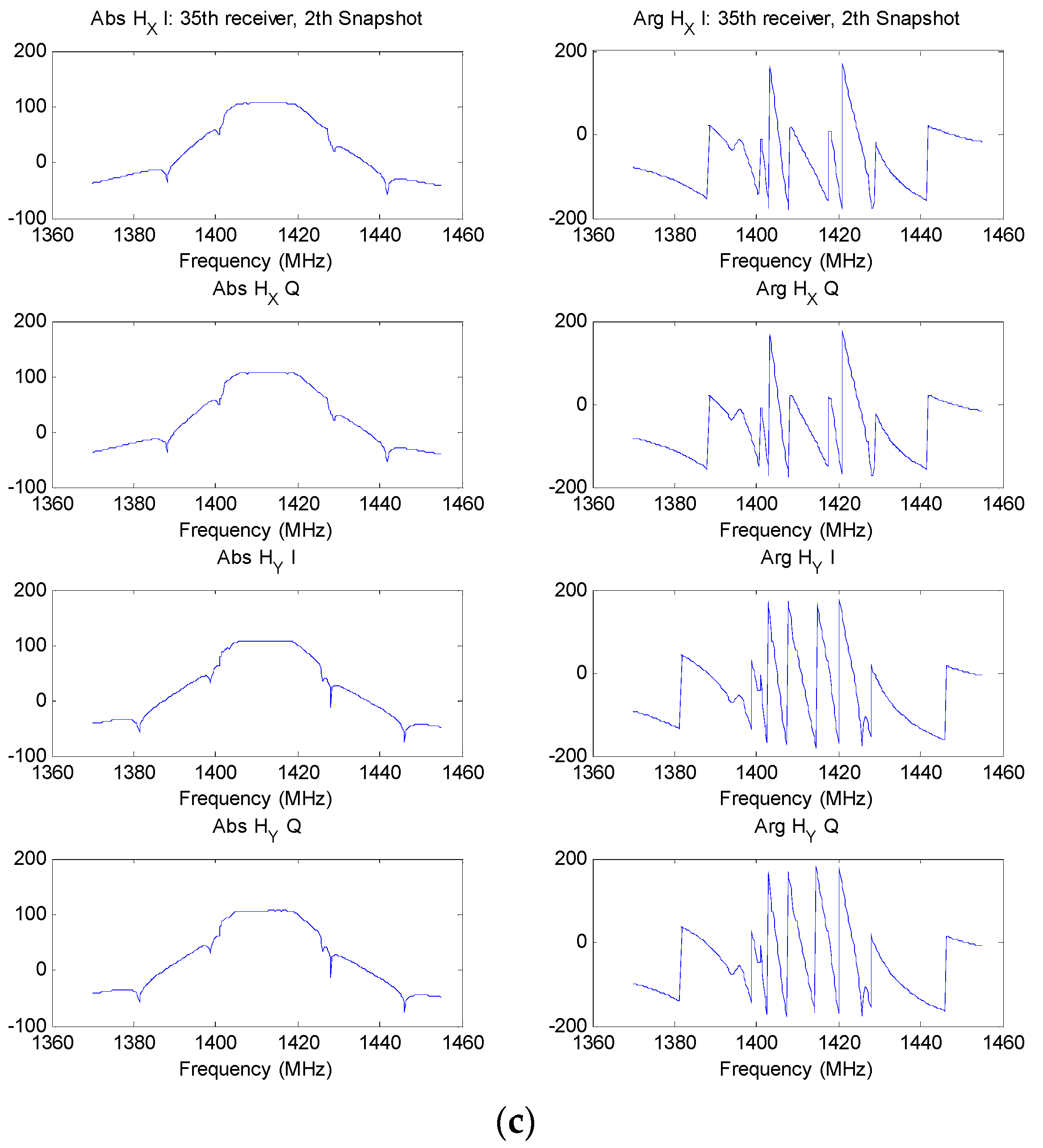
where H_{n m,n} is the frequency response of receiver m or n, respectively (I- or Q-branches), normalized to unity, and $B_{m,n}$ are the noise bandwidths. The symbol F⁻¹ is the inverse Fourier transform and u() is the step unit function. Note that the quadrature channel frequency transfer function used in ${\tilde{r}}_{mn}^{qi}$ includes a 90° phase shift introduced in the local oscillator. Figure 10 shows sample fringe-washing functions for the X- and Y-polarizations, II and QI pairs, computed using Equation (25).

An FFT algorithm is used to compute all the FWFs, and the result is limited to the main lobe of the function, which has a “sinc-like” shape. For the sake of computational efficiency in the computation of the visibility samples (“direct problem”), the fringe-wash function is approximated by:

$${\tilde{r}}_{mn}\left(\tau \right)\approx Asinc\left(B\left(\tau -C\right)\right)e^{j\left(D{\tau }^2+E\tau +F\right)}$$

(26)

The parameters A, B, C, D, E and F are computed from:

$$\left|{\tilde{r}}_{mn}\left(-T_s\right)\right|\approx Asinc\left(B\left(-T_s-C\right)\right)$$

(27a)

$$\left|{\tilde{r}}_{mn}\left(0\right)\right|\approx Asinc\left(B·C\right)$$

(27b)

$$\left|{\tilde{r}}_{mn}\left(+T_s\right)\right|\approx Asinc\left(B\left(T_s-C\right)\right)$$

(27c)

$$\text{and }D=\frac{1}{T_s^2}\left\{\frac{arg\left({\tilde{r}}_{mn}\left(+T_s\right)\right)+arg\left({\tilde{r}}_{mn}\left(-T_s\right)\right)}{2}-arg\left({\tilde{r}}_{mn}\left(0\right)\right)\right\}$$

(27d)

$$E=\frac{arg\left({\tilde{r}}_{mn}\left(+T_s\right)\right)-arg\left({\tilde{r}}_{mn}\left(-T_s\right)\right)}{2·T_s}$$

(27e)

$$F=arg\left({\tilde{r}}_{mn}\left(0\right)\right)$$

(27f)

in the image reconstruction algorithm (“inverse problem”), the fringe-wash function is estimated from calibration measurements at three different lags (−T_s, 0, T_s), mimicking the fitting in Equation (27). On the other hand, since the shape of the FWF is an even function, and the relative bandwidth is very small, it can be simply ignored and set to 1. Note that the phase and amplitude at the origin are the values that need to be calibrated.

2.1.3. Correlator Model

In the computation of the samples of the visibility function, the non-ideal digital correlator effects must also be included. Quantization distorts and spreads the cross-correlation spectrum, decreasing the radiometer resolution. Sampling also impacts the spectrum of the cross-correlation. Even above the Nyquist sampling rate, quantization spreads the spectrum. In the case of a one-bit two-level correlator, the effect is well described in the SMOS analysis [7]. More general cases are discussed in [8]. 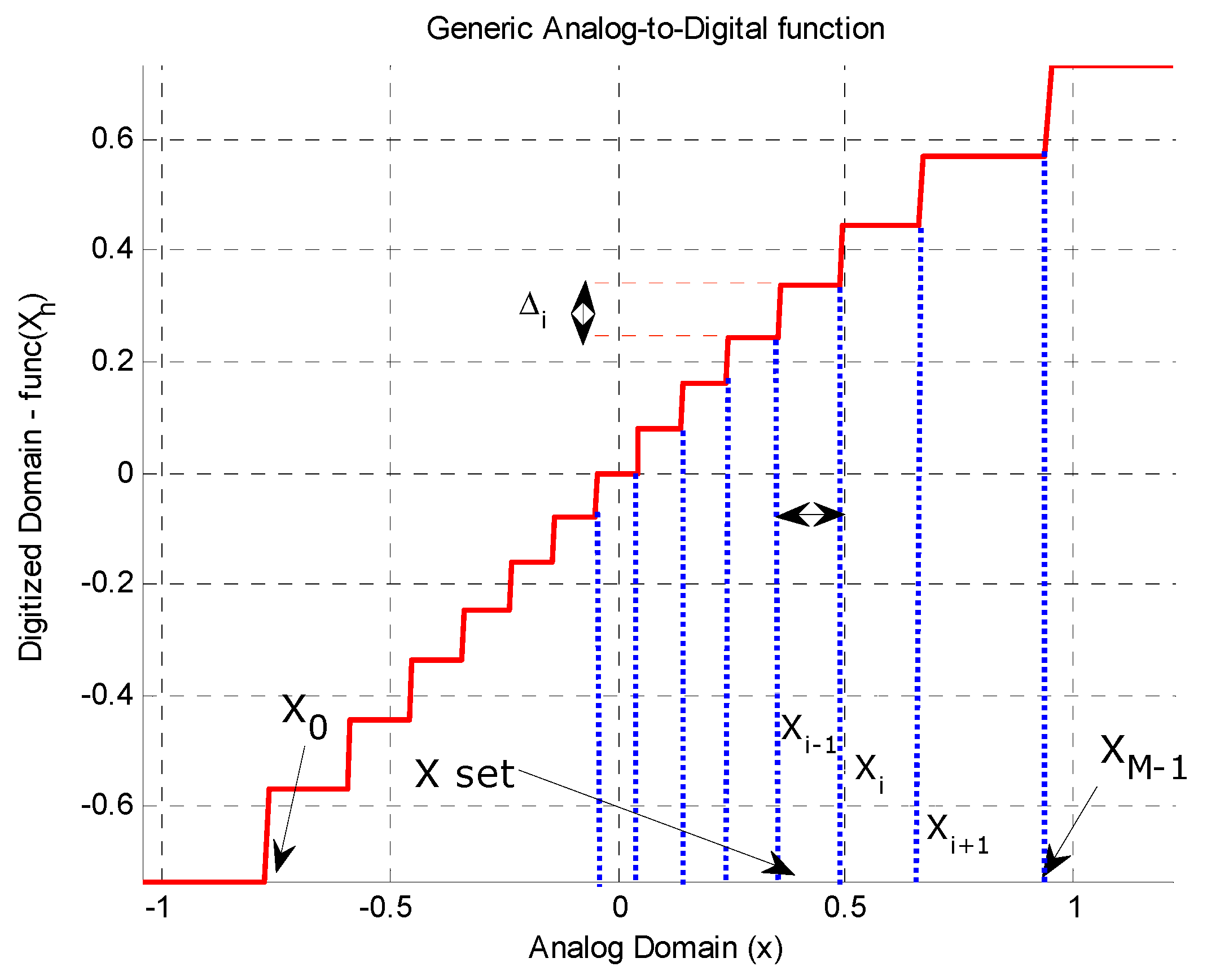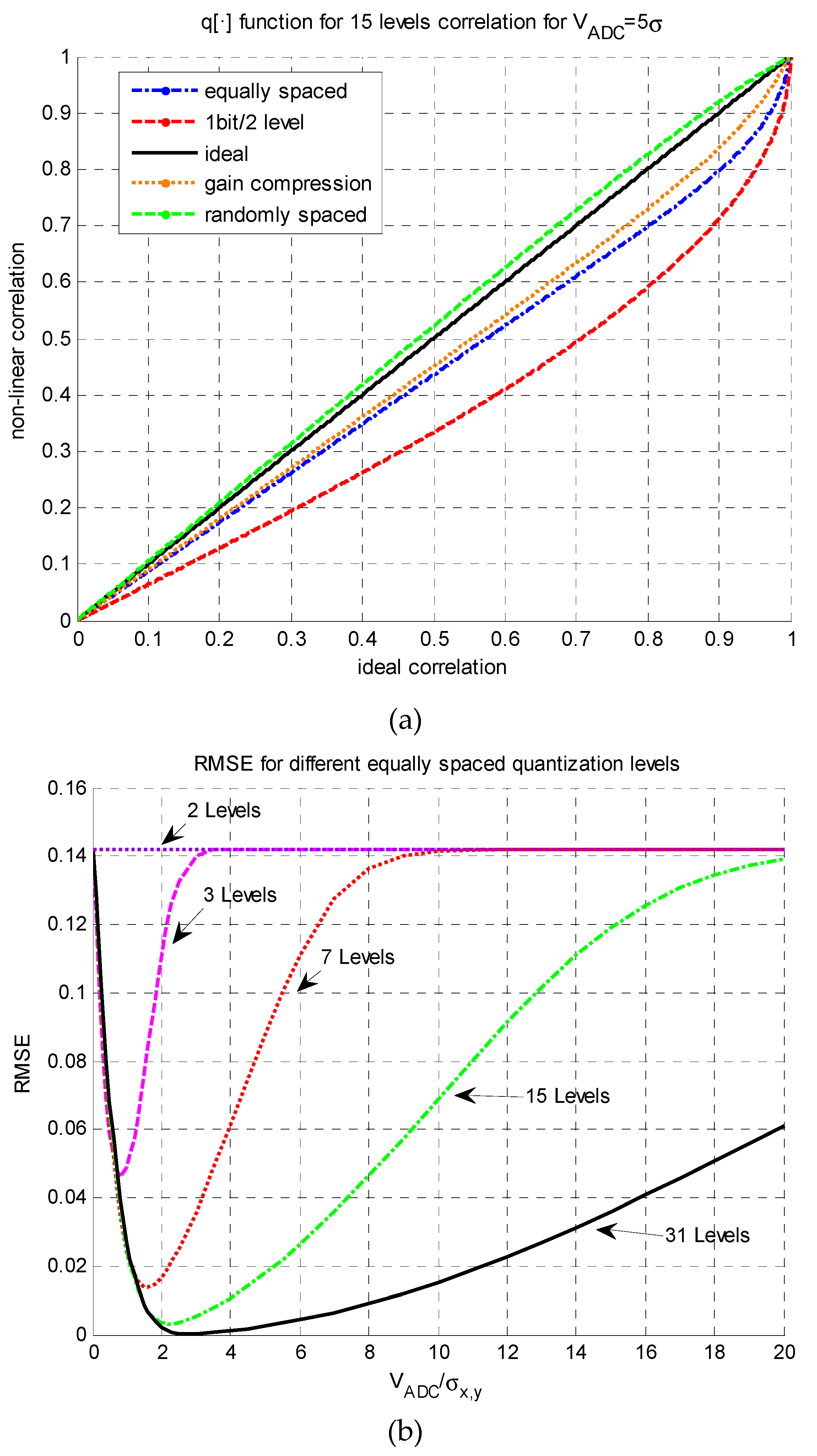Figure 11, for example, shows the transfer function g(x) of an arbitrary analog-to-digital (ADC) converter, with gain compression, and uneven spacing in the input and output variables.

The impact of quantization effects in the measured cross-correlation can be numerically computed from:

$$R_{xy}(\mathsf{\tau })=\underset{0}{\overset{{\mathsf{\rho }}_{xy}(\mathsf{\tau })}{{\displaystyle \int }}}\frac{1}{2\mathsf{\pi }\sqrt{1-{\mathsf{\rho }}_{xy}^2(\mathsf{\tau })}}{\displaystyle \sum }_{\mathrm{p}=0}^{\mathrm{P}-1}{\displaystyle \sum }_{\mathrm{q}=0}^{\mathrm{Q}-1}{\Delta }_{\mathrm{p}}^x{\Delta }_{\mathrm{q}}^y{\mathrm{e}}^{-\frac{1}{2}\frac{\left({\mathrm{X}}_{\mathrm{p}}^2+{\mathrm{Y}}_{\mathrm{q}}^2+2{\mathrm{X}}_{\mathrm{p}}{\mathrm{Y}}_{\mathrm{q}}{\mathsf{\rho }}_{xy}(\mathsf{\tau })\right)}{\left(1-{\mathsf{\rho }}_{xy}^2(\mathsf{\tau })\right)}}{\text{d}\mathsf{\rho }}_{xy}(\mathsf{\tau })$$

(28)

where ${\mathsf{\rho }}_{\text{xy}}={\mathrm{q}}^{-1}\left[R_{xy}\right]$ is the ideal correlation coefficient of the two variables x and y (before the non-linear ADC functions $g_1()$ and $g_2()$), $R_{xy}$ is the correlation coefficient of x and y after the non-linear functions $g_1()$ and $g_2()$ are applied to x and y, respectively, and X_p and Y_p are the positions where the steps of the transfer function occur (Figure 11). In some particular and simplified cases, Equation (29) can be obtained analytically, for instance in the case of quantifying with two levels (one bit, $\text{Q}=\mathrm{P}=1$ and ${\Delta }_0^x={\Delta }_0^y=2$). In this case, Equation (28) becomes the well-known solution stated [8]:

$$R_{xy}\left({\mathsf{\rho }}_{xy}(\mathsf{\tau })\right)=\frac{2}{\mathsf{\pi }}\arcsin \left({\mathsf{\rho }}_{xy}(\mathsf{\tau })\right)$$

(29)

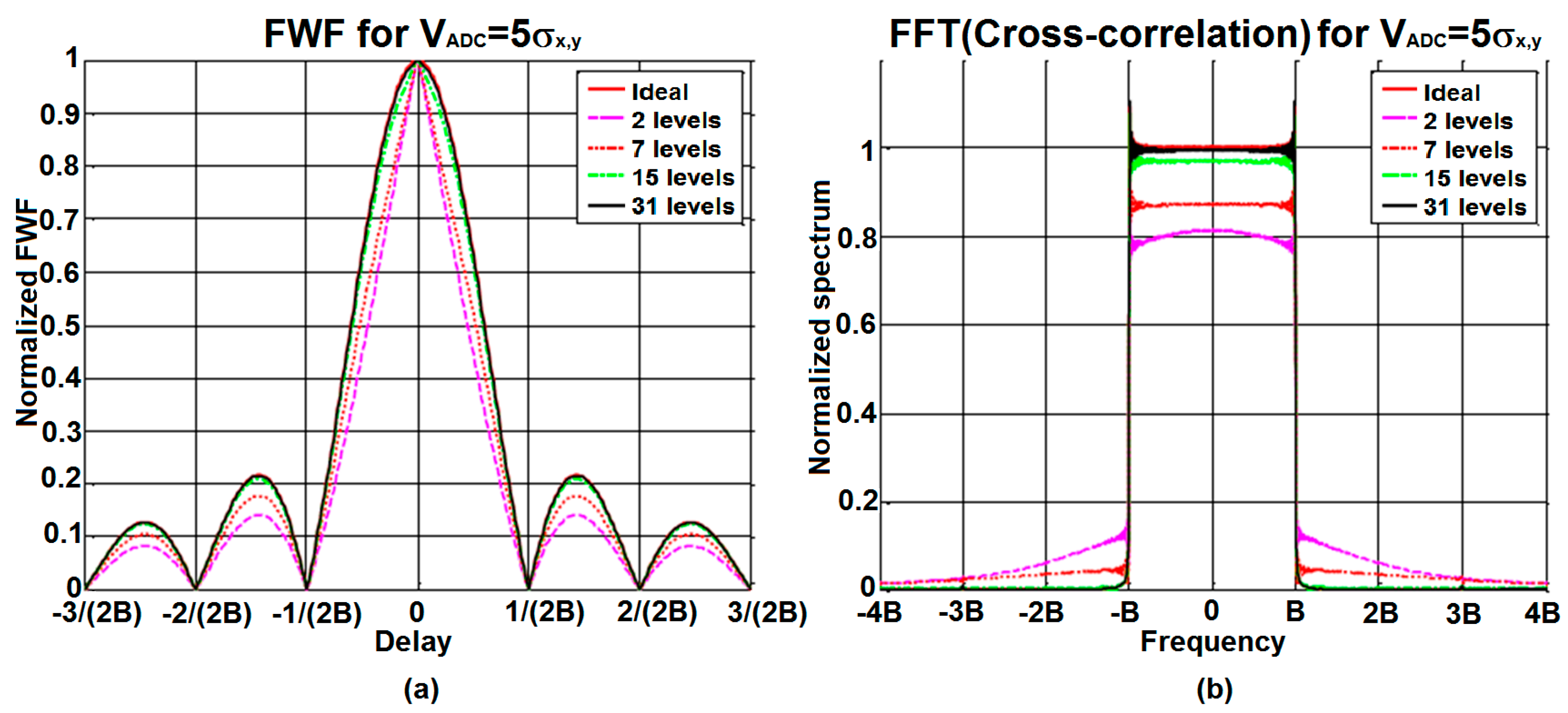
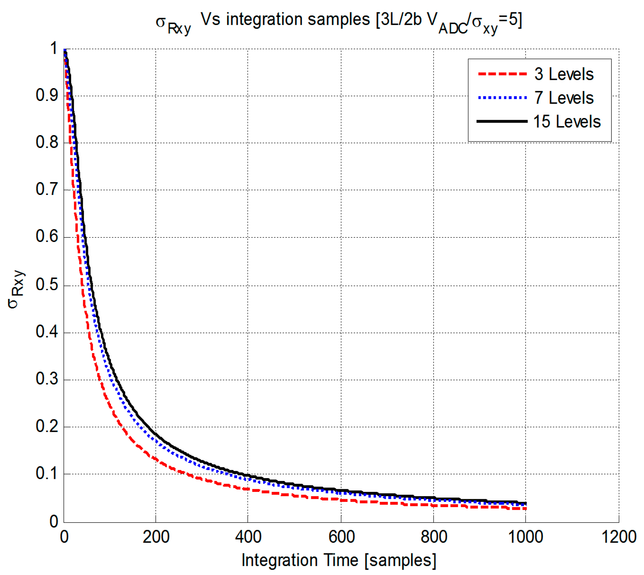
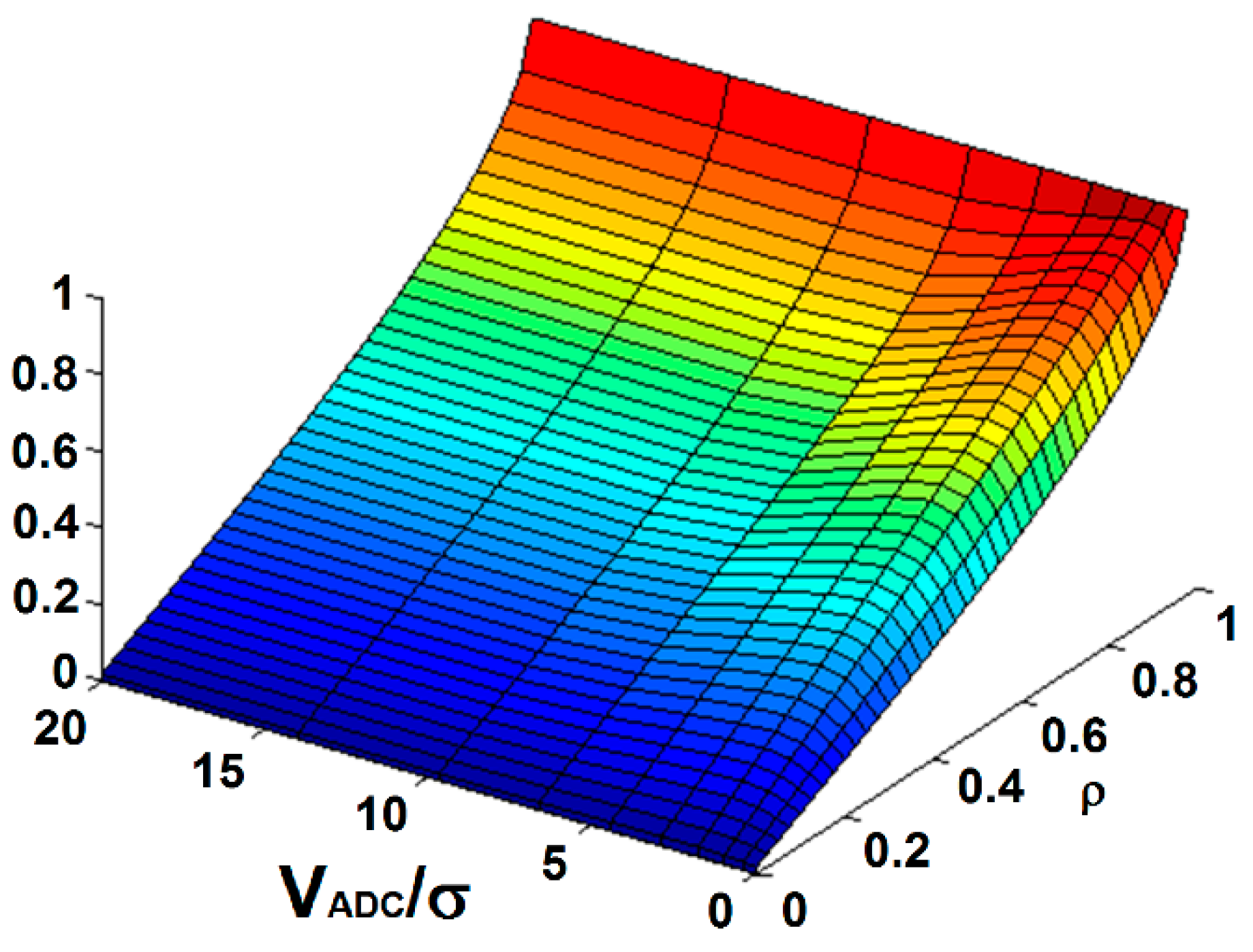
Figure 12a shows different transfer functions computed from Equation (28) for different quantization schemes using four bits (equally spaced thresholds, with gain compression or randomly distributed), one bit/two levels, and the ideal 1:1 transfer function. Figure 12b shows the root mean square error as a function of the ADC window normalized to the standard deviation of the input signals for different numbers of equally spaced quantification levels. Once the transfer functions are computed for each correlator, they are stored in look-up tables for the sake of time efficiency.

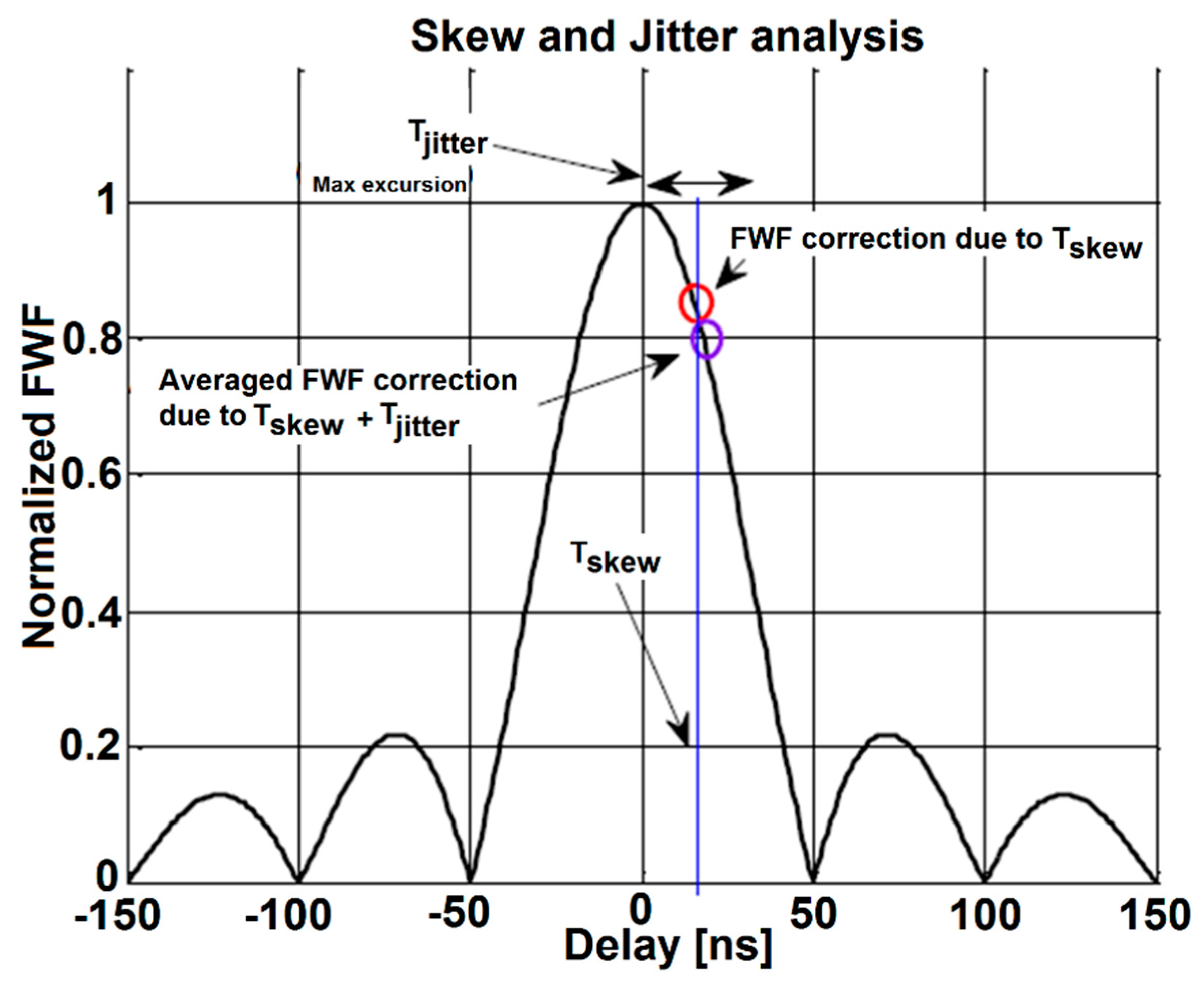
Furthermore, skew due to clock inaccuracies and jitter due to delay offset are modeled: ${\mathrm{T}}_{\text{sampling},m}-{\mathrm{T}}_{\text{sampling},n}={\mathrm{T}}_{\text{Skew}}+{\mathrm{T}}_{\text{Jitter}}\left(\mathrm{t}\right)$. The skew is a constant timing error that produces a decrease of the cross-correlation amplitude (Figure 13). Since the in-phase and quadrature branches may have (do have) different sampling errors, skew also produces a phase and quadrature error as detailed in [7]:

$${\Phi }^{\text{in}-\text{phase}}=\frac{{\Phi }^{\text{real}}+{\Phi }^{\text{imag}}}{2}={\mathsf{\pi }\text{f}}_{\text{IF}}\left({\mathrm{T}}_{\text{Skew},\text{real}}+{\mathrm{T}}_{\text{Skew},\text{imag}}\right)$$

(30a)

$${\Phi }^{\text{quadrature}}={\Phi }^{\text{real}}-{\Phi }^{\text{imag}}=2{\mathsf{\pi }\text{f}}_{\text{IF}}\left({\mathrm{T}}_{\text{Skew},\text{real}}-{\mathrm{T}}_{\text{Skew},\text{imag}}\right)$$

(30b)

where ${\mathrm{T}}_{\text{Skew},\text{real}}$ is the skew error between the I_m and I_n channels (or Q_m and Q_n) used to compute the real part of the visibility sample, and ${\mathrm{T}}_{\text{Skew},\text{imag}}$ is the skew error between the Q_m and I_n channels (or I_m and Q_n) used to compute the imaginary part of the visibility sample.

On the other hand, the jitter is a random variable effect that can be statistically modeled as a zero-mean random Gaussian variable of variance depending on time (${\mathsf{\sigma }}_{\text{Jitter}}^2={\mathsf{\sigma }}_{\text{app}}^2+{\mathrm{c}}_{\text{clk}}·\left|\mathrm{n}-\mathrm{m}\right|·{\mathrm{T}}_{\mathrm{s}}$), where “n” and “m” are two different samples. Thus, it can be associated with two different and independent processes [9,10]:

• the aperture jitter, which is related to the random sampling time variations in the ADC caused by thermal noise in the sample and hold circuit. The aperture jitter is commonly modeled as an independent Gaussian variable with zero-mean and a standard deviation of ${\mathsf{\sigma }}_{\text{Jitter}}={\mathsf{\sigma }}_{\text{app}}$.
• The clock jitter, which is a parameter of the clock generator that drives the ADC with the clock signal. The clock jitter is modeled as a Wiener process, i.e., a continuous-time, non-stationary random process with independent Gaussian increments with a standard deviation equal to ${\mathsf{\sigma }}_{\text{Jitter}}=\sqrt{{\mathsf{\sigma }}_{\text{clk}}·\left|\mathrm{n}-\mathrm{m}\right|·{\mathrm{T}}_{\mathrm{s}}}$.

Finally, jitter effects are included in the FWF as:

$${\breve{R}}_{xy}\left(\tau \right)=R_{xy}\left(\tau \right)*\frac{e^{-\frac{{\tau }^2}{2{\sigma }_{app}^2}}}{\sqrt{2\pi {\sigma }_{app}}}*\frac{e^{-\frac{\tau }{2c_{clk}}}}{\sqrt{2\pi c_{clk}\tau }}$$

(31)

where ${\breve{R}}_{xy}\left(\mathsf{\tau }\right)$ is the cross-correlation function (FWF) modified by the jitter, $R_{xy}\left(\mathsf{\tau }\right)$ is the cross-correlation function (FWF), and * denotes the convolution operator. Finally, the combined effect of skew and jitter effects can be modeled as ${\breve{R}}_{xy,real/imag}\left(T_{skew,real/imag}-\left(u·\xi +v·\eta \pm w\sqrt{1-{\xi }^2-{\eta }^2}\right)/f_0\right)$.

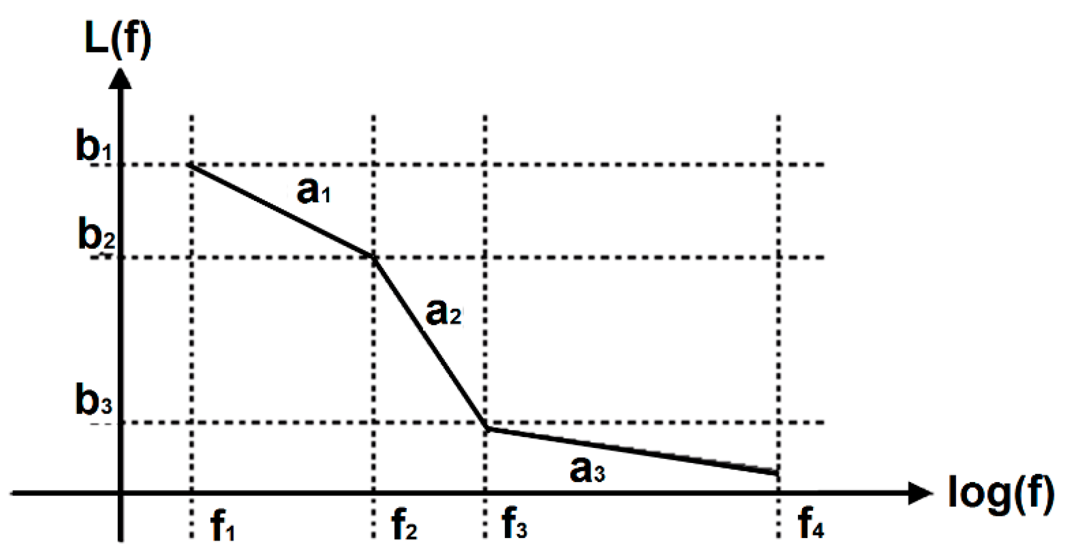
The question is now how to compute the jitter from the phase noise spectrum of the local oscillator. Figure 14 (from [11]) shows a typical phase noise spectrum, where the different areas are modeled by a constant slope term, a_i. This spectrum can be approximated by:

$$L\left(f\right)={\displaystyle \sum }_{i=1}^{K-1}\left[a_i\left(log\left(f\right)-log\left(f_i\right)\right)+b_i\right]\left[u\left(f-f_i\right)-u\left(f-f_{i+1}\right)\right]$$

(32)

where u() represents Heaviside’s step function.

The rms clock jitter (${\sigma }_{\text{Jitter}}$) can be computed as:

$${\sigma }_{jitter}=\frac{1}{2\pi f_c}\sqrt{2{\displaystyle \sum }_{i=1}^{K-1}{10}^{\frac{b_i}{10}}{f}_i^{\frac{-a_i}{10}}{{\displaystyle \int }}_{f_i}^{f_{i+1}}{f}^{\frac{a_i}{10}}df}=\frac{1}{2\pi f_c}\sqrt{2{\displaystyle \sum }_{i=1}^{K-1}{10}^{\frac{b_i}{10}}{f}_i^{\frac{-a_i}{10}}{\left(1+\frac{a_i}{10}\right)}^{-1}\left[f_{i+1}^{\frac{a_i}{10}+1}-f_i^{\frac{a_i}{10}+1}\right]}$$

(33)

The last effect that can occur is the offset induced by the local oscillator thermal noise leakage to IF through the finite LO-IF isolation. If the baseband clock is distributed, and then a dedicated Phase Locked Loop (PLL) is used in each receiver, then this effect is most likely going to be negligible, since the noises are uncorrelated. If a common LO is distributed (at least by groups), then thermal noise leaks due to the finite LO-IF isolation (>10–20 dB for a typical mixer):

$$V_{offset}=T_{ph}\frac{G}{Isolation}$$

(34)

in all channels, and therefore produces an offset at the output. In Equation (34), T_ph is the physical temperature of the LO, G is the gain of the LO driver (assuming that the LO needs to be amplified for distribution to different channels, if not G = 1), and Isolation is the LO-IF isolation of the mixer.

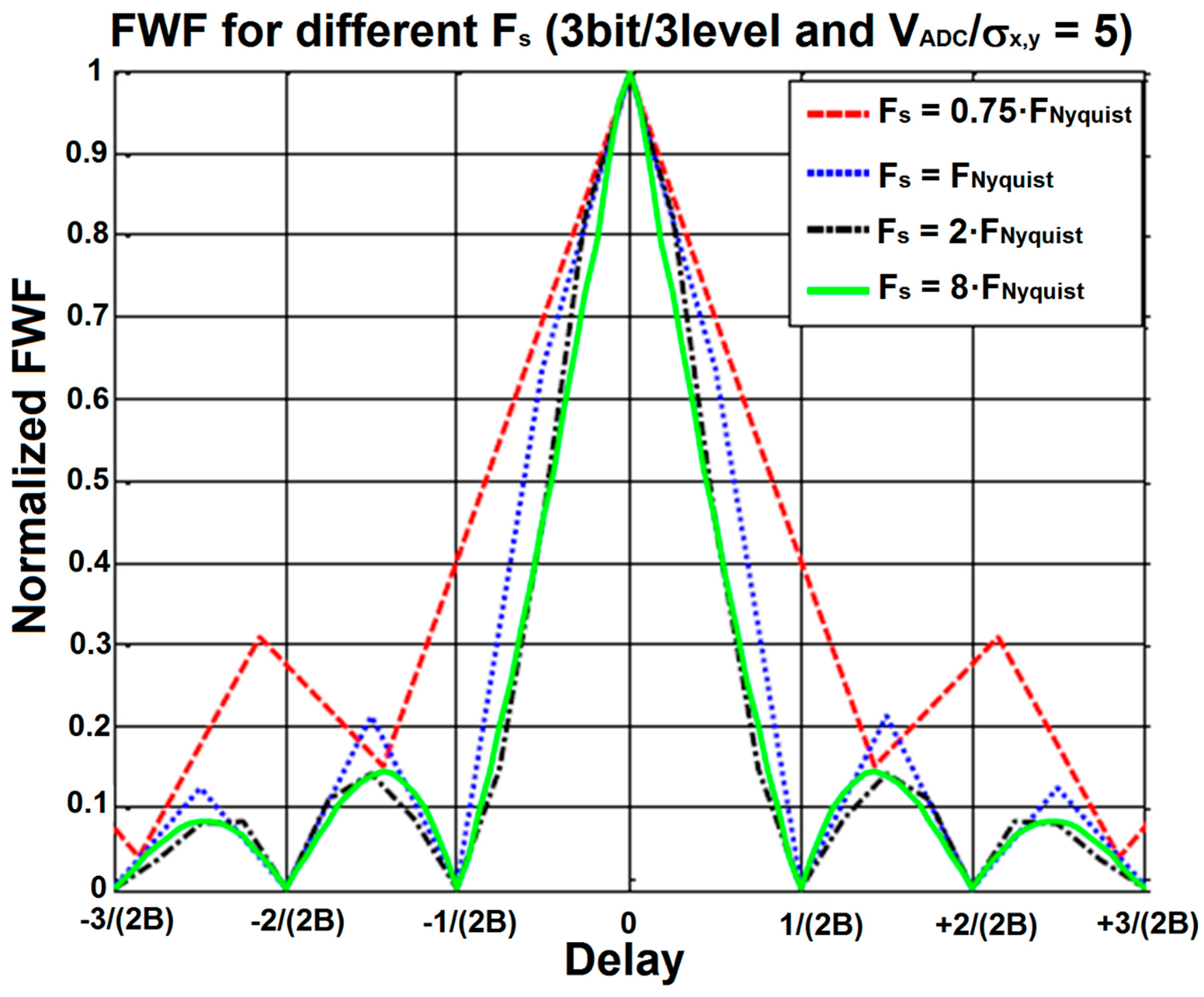
For a generic SAIR, the effect of an arbitrary type of correlator can be modeled based on the results in [12]. Figure 15a,b represent the quantization effect in the time domain (left) and its corresponding spectrum (right), which, as expected, spills above its original band. Finally, Figure 16 shows the FWF vs. sampling frequency. Note that the FWF when sampling at the Nyquist frequency, is different compared to the FWF when sampling at a much higher frequency, due to the fold-over of the “tails” of the signal’s spectrum after quantization which expand beyond $\left|f\right|\ge B$ (Figure 15b).

The thermal noise and its dependence on the correlator type are discussed below.

2.1.4. Methodology to Include Instrument Errors

Realistic Instrument Modeling

Instrument errors are already “built-in” in the calculation of the “analog” visibility samples (V(u,v) in Equation (2) which is $V\left(u,v\right)={\mathsf{\rho }}_{I_m{I}_n}^{\text{r}}+j{\mathsf{\rho }}_{Q_m{I}_n}^{\text{i}}$, since the complex cross-correlation is obtained from two real cross-correlations). Correlator errors (including quantization and sampling effects) are included in Equations (28) and (31). The thermal noise due to finite integration time (snapshot) is added directly to the real correlators’ output, R_xy ($R_{xy}=\mathrm{q}\left[{\mathsf{\rho }}_{xy}\right]$, Equation (29), with x = I_m or Q_m, and y = I_n). The addition of thermal noise applies both in observation and noise injection modes.

Uncorrelated Noise Model

The value of the variance of the correlation obtained after averaging $N_q$ samples (N quantized samples) is given by [12]:

$${\sigma }_{R_{xy}}^2=\frac{{\sigma }_{g_m\left(x\right)}^2{\sigma }_{g_n\left(y\right)}^2}{N_q}+\frac{2}{N_q^2}{\displaystyle \sum }_{n=1}^{N_q}\left(N_q-n\right)R_{xx}\left(n{\mathrm{T}}_s\right)R_{yy}\left(n{\mathrm{T}}_s\right)$$

(35)

where ${\sigma }_{g_m\left(x\right)}^2$ and ${\sigma }_{g_n\left(y\right)}^2$ are the variances for each sample of the correlation, and $R_{xx}\left(n{\mathrm{T}}_s\right)$ and $R_{yy}\left(n{\mathrm{T}}_s\right)$ are the auto-correlations of $g_m\left(x\right)$ and $g_n\left(y\right)$. For simplicity, it is assumed that all ADCs are the same type, although they can have different random errors, so g = g_m = g_n, and ${\sigma }_{g_m\left(x\right)}^2={\sigma }_{g_n\left(y\right)}^2$.

In Figure 17, the evolution of the standard deviation of the cross-correlation (${\mathsf{\sigma }}_{{\mathrm{R}}_{\text{xy}}}$) as a function of the number of samples N_q for three and 15 levels, with sampling at exactly the Nyquist rate, is presented. The three-level curve converges more quickly to zero than the 15-level curve, because the shape of the FWF is sharper due to the higher non-linear distortion at the three-level than at the 15-level quantization. This effect is equivalent to having more uncorrelated samples. Despite the mean of the correlation being lower for the three-level than the 15-level quantization, the variance of the correlation is also lower in this case.

In Equation (35), in the case of an infinite number of bits and $F_s\ge F_{Nyquist}$, N_q = N = B·τ, where N is the total number of uncorrelated samples, B is the noise bandwidth, and τ is the integration time. The evaluation of Equation (35) may be impractical from the implementation point of view, due to excessive time spent in the evaluation of the summation. In [8], the concept of effective integration time is used:

$$N_q\triangleq B·{\tau }_{eff}$$

(36)

with ${\tau }_{eff}=\tau /C$ being C a function of the correlator type and the sampling frequency normalized to the Nyquist sampling frequency [8].

Using this approach, the noise will be added to Equation (2) as a zero-mean random variable with standard deviation equal to that of the noise:

$${\sigma }_{r,i}=\frac{1}{\sqrt{2B{\tau }_{eff}}}$$

(37)

Finally, thermal noise has to be added to the zero baseline as well. The zero baseline (the antenna temperature at a given polarization) is not measured as a cross-correlation, but using a dedicated total power radiometer or power measurement system (diode detector) in each branch of the receivers. The noise computation follows the standard formulas, for example in [13].

Correlated Noise Model

There is correlation in the noise of the measured visibility samples [14]. If $\overrightarrow{\text{n}}$ is a noise vector, a realization of an independent unit-variance complex circular Gaussian noise, it can be transformed into a cross-correlated noise vector by the Cholesky factorization of the cross-correlation matrix ($\stackrel{=}{\mathrm{C}}$):

$${\overrightarrow{\text{n}}}_{\mathrm{V}}=\stackrel{=}{\mathrm{R}}·\overrightarrow{\text{n}}$$

(38a)

$$\stackrel{=}{\mathrm{C}}={\stackrel{=}{\mathrm{R}}}^{\mathrm{H}}·\stackrel{=}{\mathrm{R}}$$

(38b)

where the elements of $\stackrel{=}{\mathrm{C}}$ are given by:

$${\mathrm{c}}_{mn}=\frac{1}{B·\tau }·\{\begin{array}{c}{\mathrm{V}}_{km}·{\mathrm{V}}_{ln}^{*},k\ne m,l\ne n,\\ {\mathrm{V}}_{km}·{\mathrm{V}}_{ln}^{*}+{\mathrm{T}}_{\mathrm{R},l}·{\mathrm{V}}_{km},k\ne m,l=n,\\ {\mathrm{V}}_{km}·{\mathrm{V}}_{ln}^{*}+{\mathrm{T}}_{\mathrm{R},k}·{\mathrm{V}}_{ln},k=m,l\ne n,\\ {\mathrm{V}}_{km}·{\mathrm{V}}_{ln}^{*}+{\mathrm{T}}_{\mathrm{R},l}·{\mathrm{V}}_{km}+{\mathrm{T}}_{\mathrm{R},k}·{\mathrm{V}}_{ln}+{\mathrm{T}}_{\mathrm{R},k}·{\mathrm{T}}_{\mathrm{R},l},k=m,l=n\end{array}$$

(38c)

To take into account the effect of the correlator type and sampling frequency, the integration time must correspond to the effective integration time ${\tau }_{eff}$ [8]. The Cholesky decomposition requires a lot of computational resources, and is impractical for large array sizes of the SAIR.

In the nominal case, the thermal noise due to finite integration time (snapshot) is added directly to visibilities as a zero-mean random variable with standard deviation equal to that of the noise:

$${\mathsf{\sigma }}_{\mathrm{r},\mathrm{i}}^2=\left\{\frac{1}{2B·{\tau }_{eff}}+{\left(\frac{{\Delta \text{G}}_m}{{\mathrm{G}}_m}\right)}^2+{\left(\frac{{\Delta \text{G}}_n}{{\mathrm{G}}_n}\right)}^2\right\}·\{\left({\mathrm{T}}_{\mathrm{A},m}+{\mathrm{T}}_{\mathrm{R},m}\right)\left({\mathrm{T}}_{\mathrm{A},n}+{\mathrm{T}}_{\mathrm{R},n}\right)·\left[1+\mathsf{\Lambda }\left(\frac{2\Delta \text{f}}{\mathrm{B}}\right)\right]+{\mathrm{V}}_{\mathrm{r},\text{i }mn}^2·\left[1+\mathsf{\Lambda }\left(\frac{2\Delta \text{f}}{\mathrm{B}}\right)\right]-{\mathrm{V}}_{\mathrm{i},\text{r }mn}^2·\left[1-\mathsf{\Lambda }\left(\frac{2\Delta \text{f}}{\mathrm{B}}\right)\right]\}$$

(39)

where T_A and T_R are the antenna temperature and receiver’s noise temperature, and $\Delta \text{f}={\mathrm{f}}_0-{\mathrm{f}}_{\text{LO}}$, where ${\mathrm{f}}_0$ is the central frequency and ${\mathrm{f}}_{\text{LO}}$ is the local oscillator frequency, B is the receivers’ noise bandwidth, and the triangle function is defined as $\mathsf{\Lambda }\left(x\right)=1-\left|x\right|;\left|x\right|\le 1$.

Simplified Instrument Modeling

Furthermore, to test the impact of each individual error source in the radiometric resolution, it may be interesting not to perform the realistic calibration and instead use an “ideal” image reconstruction approach, consisting basically of an inverse Fourier transform, followed by an average antenna pattern and obliquity factor compensation. The “ideal” image reconstruction neglects all the instrument error modeling (Equation (2)) and assumes that antenna patterns are all equal for all elements, and the fringe-wash function is the same for all baselines.

The errors that can be used as an input are: amplitude errors (${\mathsf{ϵ}}_{\mathrm{A}}$: mean value + zero-mean Gaussian random variable determined by its standard deviation N(0, σ_A)), phase errors (${\mathsf{ϵ}}_{\mathsf{\varphi }}$: mean value + zero-mean Gaussian random variable determined by its standard deviation N(0, σ_ϕ) or a uniform random variable from −π to +π: U(−π, +π)), and offset errors (${ϵ}_{offset,r}$ and ${ϵ}_{offset,i}$: mean value + zero-mean Gaussian random variable determined by its standard deviation for the real and imaginary parts N(0, ${\sigma }_{V_{offset,r}}$) and N(0, ${\sigma }_{V_{offset,i}}$)). Antenna co- and cross-polar pattern errors include a model for a sinusoidal oscillation of amplitude and phase equal to zero-mean Gaussian random variables determined by their standard deviations.

To summarize, the starting point will be Equation (2), but with all FWFs being the same $\tilde{\text{r}}\left(\Delta \text{t}\right)=\text{sinc}\left(\mathrm{B}·\Delta \text{t}\right)$, and errors being added as:

$$\mathrm{V}\left(u,v\right)=\left(1+{\mathsf{ϵ}}_{\mathrm{A}}\right)·{\mathrm{e}}^{\mathrm{j}{\mathsf{ϵ}}_{\mathsf{\varphi }}}·\left\{{\mathrm{V}}_{\mathrm{r}}\left(u,v\right)+\mathrm{j}·{\mathrm{V}}_{\mathrm{i}}\left(u,v\right)\right\}+\left\{{\mathsf{ϵ}}_{\text{offset},\text{r}}+\mathrm{j}·{\mathsf{ϵ}}_{\text{offset},\text{i}}\right\}$$

(40)

2.2. Modeling of Instrument Calibration

The correction of instrumental errors in a SAIR can be performed using internal and external calibrators. Internal calibration consists of commuting the input switch to signals with known correlations, such as (1) matched loads producing uncorrelated noise, and therefore (ideally) zero visibilities; and (2) correlated noise generated by a common noise source and distributed through a power splitter, therefore producing (ideally) known non-zero visibilities. External calibration consists of the measurement of known BT scenes such as homogeneous ones (e.g., the flat target response) or quasi-point sources. Other calibration techniques based on properties of the visibility samples can be used, such as the redundant space calibration or the phase/amplitude closures. These techniques are described below.

2.2.1. Internal Calibration

Calibration by Noise Injection (NI)

Figure 18 below shows the diagram flow of the calibration for noise injection in centralized noise injection. During the calibration, the Instrument module (Section 2.1) simulates all the instrument modes and generates the following data: correlations (digital counts) and power measurement system (PMS) gains and voltages for the uncorrelated and correlated noise injection modes, and for the science mode (input switch connected to the antenna).

The calibration procedure first processes the correlated noise injection data to estimate the FWF at the origin and the calibrated PMS (power measurement system) gains and offsets. Then, the uncorrelated noise data is processed to compute the visibilities offsets. Finally, the science data is calibrated with the previously computed parameters.

In order to model the drifts of the calibrators themselves, average values, standard deviations and temperature drifts of the noise sources, the S-parameters of the distribution network, and the parameters of the PMS used to estimate the baseline at the origin (as total power radiometers) are accounted for. Since the approach of this project is to simulate arbitrary SAIRs, specific noise injection approaches, such as the distributed one in SMOS [15], are not feasible to implement; therefore, the noise distribution network is simulated using the S-parameters of an ideal 1:N power splitter, with some random errors added on top of these ideal values. The values of the S-parameters of this “ideal” power splitter will be: ${\left|{\mathrm{S}}_{0m}\right|}^2={\left|{\mathrm{S}}_{m0}\right|}^2=1/\mathrm{N},m:1\dots \mathrm{N}$, ${\left|{\mathrm{S}}_{mm}\right|}^2=0,m=0\dots \mathrm{N}$; and ${\left|{\mathrm{S}}_{mn}\right|}^2=0,m,n=1\dots \mathrm{N}$.

PMS Calibration

The PMS system will measure system temperatures through the relationship:

$$v_m=v_{m,offset}+G_m·T_{sys,m}$$

(41)

where $T_{sys,m}$ is the system temperature of the mth receiver and it has already been previously computed from the receivers’ noise temperature and the “antenna temperature” or the noise temperature being injected. During internal noise injection calibration, the following four voltages are computed, for two input system temperatures ($T_{sys,m}^{WARM}$ and $T_{sys,m}^{HOT}$) and for two receiver gains (with and without attenuator $L_m$ in the receiving path), and including errors in the noise source temperatures:

$$v_{1,m}=v_{offset,m}+G_m·T_{sys,m}^{WARM}$$

(42a)

$$v_{2,m}=v_{offset,m}+G_m·T_{sys,m}^{HOT}$$

(42b)

$$v_{3,m}=v_{offset,m}+\frac{G_m}{L_m}·T_{sys,m}^{WARM}$$

(42c)

$$v_{4,m}=v_{offset,m}+\frac{G_m}{L_m}·T_{sys,m}^{HOT}$$

(42d)

This technique is known as the four-point method, and allows us to compute the PMS gains and offsets as [16]:

$$v_{offset,m}=\frac{v_{2,m}·v_{3,m}-v_{1,m}·v_{4,m}}{\left(v_{2,m}-v_{4,n}\right)-\left(v_{1,m}-v_{3,n}\right)}$$

(43a)

$$G_m=\frac{v_{2,m}-v_{1,m}}{T_{sys,m}^{HOT}-T_{sys,m}^{WARM}}$$

(43b)

Visibilities Denormalization

From the PMS voltages and the PMS computed gain and voltage offset (Equation (43a,b)), the system temperatures can be computed and multiplied to the observables being processed.

Correlator Transfer Inversion

For a homogenous processing of the visibility samples, regardless of the number of bits of the complex cross-correlators, the normalized cross-correlations (µ_mn) are defined as the actual cross-correlation (either analog ρ_xy or digital R_xy) divided by the product of the standard deviation of the two signals being cross-correlated (σ_x·σ_y). Then, the inverse of the correlator transfer function (Equation (28) and Figure 12a) is performed, averaging the number of ADC sigma levels, the reference correlator function is computed in the instrument simulation.

Quadrature Error Correction

The quadrature error is computed for all instrument modes and applied before any other processing is performed. It is corrected by multiplying the vector formed by the real and imaginary parts of the normalized visibility by the inverse of the quadrature-error matrix, which for baseline m-n is given by:

$${\stackrel{=}{M}}_{mn}=\left[\begin{array}{ll}+\cos \left(-\frac{{\theta }_{q,m}}{2}+\frac{{\theta }_{q,n}}{2}\right)& +\sin \left(-\frac{{\theta }_{q,m}}{2}+\frac{{\theta }_{q,n}}{2}\right)\\ -\sin \left(+\frac{{\theta }_{q,m}}{2}+\frac{{\theta }_{q,n}}{2}\right)& +\cos \left(+\frac{{\theta }_{q,m}}{2}+\frac{{\theta }_{q,n}}{2}\right)\end{array}\right]$$

(44)

Quadrature errors ${\mathsf{\theta }}_{q,m}$ are computed from the cross-correlation of the in-phase and quadrature signals of the same receiving element (m) at a zero delay.

FWF at the Origin

The purpose of this function is to compute the fringe-wash function at the origin (or at given time delays when observables are available), applying the following expression:

$$g_{m,n}\left(0\right)=\frac{{\mu }_{m,n}^{HOT}·\sqrt{\left(v_{2,m}-v_{\text{offset},m}\right)·\left(v_{2,n}-v_{\text{offset},n}\right)}-{\mu }_{m,n}^{WARM}·\sqrt{\left(v_{1,m}-v_{\text{offset},m}\right)·\left(v_{1,n}-v_{\text{offset},n}\right)}}{\sqrt{\left(v_{2,m}-v_{1,m}\right)·\left(v_{2,n}-v_{1,n}\right)}}$$

(45a)

where the normalized visibilities during the WARM and HOT noise injection are given by:

$${\mu }_{mn}^{HOT}=\frac{S_{m,0}·S_{n,0}^{*}\left(T^{HOT}-T_{ph}^{NDN}\right)}{\sqrt{T_{sys,m}^{HOT}·T_{sys,n}^{HOT}}}$$

(45b)

$${\mu }_{mn}^{WARM}=\frac{S_{m,0}·S_{n,0}^{*}\left(T^{WARM}-T_{ph}^{NDN}\right)}{\sqrt{T_{sys,m}^{WARM}·T_{sys,n}^{WARM}}}$$

(45c)

and $T^{HOT}$ and $T^{WARM}$ are the HOT and WARM noise temperatures at the input of the noise distribution network, $T_{ph}^{NDN}$ is the physical temperature of the noise distribution network, and $S_{m,0},S_{n,0}$ are the S-parameters of the power splitter from the input port “0” to the output ports “m” and “n”.

The amplitude of the fringe-washing function at τ = 0 along with the above remaining phase form a complex constant which will be used to divide (denormalize) the normalized visibility samples in the error correction module.

FWF Shape Computation

The FWF at the origin, $g_{mn}\left(0\right),$ is used to denormalize the calibrated visibilities, while the values at ±τ are used to compute the FWF approximation (Equations (26) and (27)). The expression used to compute the FWF at three time delays will be:

$${\overline{g}}_{mn}\left(-\tau \right)=\frac{g_{mn}\left(-\tau \right)}{g_{mn}\left(0\right)}·e^{+j2\pi f_{IF}\tau }$$

(46a)

$${\overline{g}}_{mn}\left(0\right)=1$$

(46b)

$${\overline{g}}_{mn}\left(+\tau \right)=\frac{g_{mn}\left(+\tau \right)}{g_{mn}\left(0\right)}·e^{-j2\pi f_{IF}\tau }$$

(46c)

2.2.2. External Calibration

Calibration by Redundant Space Calibration (RSC)

This calibration technique is based on the fact that the same baselines must measure the same value, and if not, this difference can be attributed to separable amplitude and phase errors, meaning errors that can be associated with each receiving chain [17]. Therefore, this technique can only be applied to regular arrays, and preferably to the already calibrated non-normalized visibility samples, to correct for the separable phase/amplitude error terms associated with the path between the antenna reference plane to the input switch. This technique cannot be applied to arrays with arbitrary shape or moving arrays, since the number of redundant baselines may be very limited (if any).

The RSC is based in the fact that in the presence of separable instrumental phase/amplitude errors, the phase/amplitude of the measured visibility samples can be related to the phase of the ideal visibility. Assuming that each array element has a phase error fm and an amplitude error gm, the phase ${\varphi }_{mn}^{raw}$ and amplitude $\left|V_{mn}^{raw}\right|$ of the measured complex cross-correlation $V_{mn}^{raw}$ are given by:

$${\varphi }_{mn}^{raw}=f_m-f_n+{\varphi }_{mn}^{id}$$

(47a)

$$\left|V_{mn}^{raw}\right|=g_m{g}_n\left|V_{mn}\right|$$

(47b)

Equation (47b) can be linearized by taking the natural logarithms on both sides of the equation:

$$ln\left(\left|V_{mn}^{raw}\right|\right)=\ln \left(g_m\right)+\ln \left(g_n\right)+ln\left(\left|V_{mn}\right|\right)$$

(48a)

or equivalently:

$$A_{mn}^{raw}=G_m+G_n+A_{mn}$$

(48b)

with the obvious definitions $G_{m,n}\widehat{=}\ln \left(g_{m,n}\right)$, $A_{mn}^{raw}=ln\left(\left|V_{mn}^{raw}\right|\right)$ , and $A_{mn}=ln\left(\left|V_{mn}\right|\right)$.

Since the spatial cross-correlation is only a function of the antenna separation, all the antennas spaced the same distance in the same direction measure the same baseline (u, v, w), which is called a redundant baseline. The information contained in redundant baselines (Equation (47a,b)) allows us to define a system of equations that can be solved for f_m,n and $g_{m,n}$. Without loss of generality the phases and amplitudes of all elements can be referred to as an arbitrary arm antenna “i”, whose phase is set to zero (f_i = 0), and its amplitude to one (g_i = 1, G_i = 0).

Calibration by Phase/Amplitude Closures

When the antenna positions are such that no redundant baselines exist, or they are moving, the redundant space calibration cannot be applied. In this case, a series of mathematical relationships linking the phase of the measured (“raw”) and the “ideal” visibility samples can be derived.

According to Equation (47a), the sum of the phases of three visibilities forming a triangle is given by:

$${\varphi }_{pq}^{raw}=f_p-f_q+{\varphi }_{pq}$$

(49a)

$${\varphi }_{qr}^{raw}=f_q-f_r+{\varphi }_{qr}$$

(49b)

$${\varphi }_{rp}^{raw}=f_r-f_p+{\varphi }_{rp}$$

(49c)

$${\varphi }_{pq}^{raw}+{\varphi }_{q,r}^{raw}+{\varphi }_{rp}^{raw}={\varphi }_{pq}+{\varphi }_{qr}+{\varphi }_{rp}$$

(49d)

Similarly, according to Equation (47b) for the amplitudes:

$$\left|V_{mn}^{raw}\right|=g_m{g}_n\left|V_{mn}\right|$$

(50a)

$$\left|V_{pq}^{raw}\right|=g_p{g}_q\left|V_{pq}\right|$$

(50b)

$$\left|V_{mp}^{raw}\right|=g_m{g}_p\left|V_{mp}\right|$$

(50c)

$$\left|V_{nq}^{raw}\right|=g_n{g}_q\left|V_{nq}\right|$$

(50d)

$$\frac{\left|V_{mn}^{raw}\right|\left|V_{pq}^{raw}\right|}{\left|V_{mp}^{raw}\right|\left|V_{nq}^{raw}\right|}=\frac{\left|V_{mn}\right|\left|V_{pq}\right|}{\left|V_{mp}\right|\left|V_{nq}\right|}$$

(50e)

Defining two systems of equations, one for all phase closures (Equation (49d)) and another one for the logarithms of all amplitude closures (Equation (50e) then becomes a linear equation), and solving by a least squares procedure, the visibilities’ amplitudes and phases are estimated. Then, when the visibilities are well calibrated, except for the measurement noise, Equation (49d) should be close to 0, and Equation (50e) close to 1. Figure 19 shows the graphical representation of these mathematical relationships.

Calibration Using External Sources

When the instrument is imaging a very bright point source at a direction $\left({\xi }_0,{\eta }_0\right)=\left(sin{\theta }_{0}cos{\phi }_0,sin{\theta }_{0}sin{\phi }_0\right)$, such that its angular extension is much smaller than the angular resolution of the instrument and the background can be neglected, all visibility samples must have the same amplitude, and the phase must be $\varphi \left(u,v\right)=-2\pi \left(u{\xi }_0+v{\eta }_0\right)$. This allows us to immediately perform a relative calibration by multiplying the measured visibility samples by the following calibration factor:

$$C=\frac{1}{\left|V\left(u,v\right)\right|}{e}^{-j\left\{arg\left(V\left(u,v\right)\right)+2\pi \left(u{\xi }_0+v{\eta }_0\right)\right\}}$$

(51)

although absolute calibration would only be possible if the intensity of the point source is known.

If the point source has a finite extension, such as the disk of the sun, an analytical model for the visibilities can be derived and included in Equation (51). Figure 20 shows the visibilities computed for a quasi-point source. The amplitude should be constant because of the Fourier transform relationship between the input BT image and the visibility samples; however, it is not perfectly constant since the input is a quasi-point source, and because of the simulated “measurement” noise. Only the zero baseline that contains the receiver temperature to be used in the image reconstruction routines is different.

The Flat Target Transformation

The flat target transformation relies on the measurement of a known and spatially constant BT scene ($T_B\left(\xi ,\eta \right)=T_{B0})$ so that the “offset” term in Equation (2) and the imperfect antenna pattern knowledge can be assessed [18]. Equation (52a,b) below are identical to Equation (2a,b), except that $T_B\left(\xi ,\eta \right)$ has been replaced by $T_{B0}$:

$$V_{r,0}\left(u,v\right)=Re\left[\frac{1}{\sqrt{{\mathsf{\Omega }}_m{\mathsf{\Omega }}_n}}\underset{{\xi }^2+{\eta }^2\le 1}{{\displaystyle \iint }}\frac{T_{B0}-T_{REC}}{\sqrt{1-{\xi }^2-{\eta }^2}}{F}_{n,m}\left(\xi ,\eta \right)F_{n,n}^{*}\left(\xi ,\eta \right){\tilde{r}}_{mn}^{ii}\left(\Delta t\right)e^{jk\Delta r}d\xi d\eta \right]$$

(52a)

$$V_{i,0}\left(u,v\right)=Im\left[\frac{1}{\sqrt{{\mathsf{\Omega }}_m{\mathsf{\Omega }}_n}}\underset{{\xi }^2+{\eta }^2\le 1}{{\displaystyle \iint }}\frac{T_{B0}-T_{REC}}{\sqrt{1-{\xi }^2-{\eta }^2}}{F}_{n,m}\left(\xi ,\eta \right)F_{n,n}^{*}\left(\xi ,\eta \right){\tilde{r}}_{mn}^{qi}\left(\Delta t\right)e^{jk\Delta r}d\xi d\eta \right]$$

(52b)

By properly scaling $V_{r,0}\left(u,v\right)$ and $V_{i,0}\left(u,v\right)$ by $T_{B0}-T_{REC}$, and multiplying it by $\overline{T_B}-T_{REC}$ (during the subsequent measurements, $\overline{T_B}$ being the average brightness temperature in the scene, see Equation (53g)), the impact of the antenna patterns and $T_{REC}$ is canceled. This calibration affects the offsets in the visibility samples induced by the antenna coupling, but it requires a prior amplitude and phase calibration, by, e.g., centralized noise injection, or using external point sources.

Figure 21 shows the visibility samples as measured by a Y-shaped array, corresponding to a flat target, a $\sqrt{cos\left(\theta \right)}$ antenna voltage pattern to compensate the obliquity factor, and FWF equal to one. Ideally, the visibilities of a flat constant input BT image should look like an impulse response because of the Fourier transform relationship. However, because the spatial frequencies (baselines) are not infinite, the output visibilities samples exhibit a sort of sinc-like shape with rotational symmetry with a sharp peak.

2.3. Image Reconstruction Algorithms

The image reconstruction algorithms ingest the calibrated visibilities and auxiliary data such as the antenna voltage patterns, the antenna positions and orientations, and the estimated FWFs, and they compute the reconstructed BT maps in all selected polarizations (either XX and YY or the four Stokes elements in the antenna reference frame).

Before the image reconstructions algorithms are applied, a number of pre-processing steps are required:

• Compensation of Polarization Rotation

The purpose of this function is to correct the different antenna polarization rotations in the input visibilities, setting all to the instrument polarization reference frame by inverting either Equation (6) in a fully polarimetric instrument, or Equation (7) (if not singular) in a dual-polarization instrument.

• A Priori BT Compensation

This procedure was first proposed in [19,20] to minimize the ringing introduced in the reconstruction by the Gibbs phenomenon due to the sharp transition between the Earth and cold sky background, by subtracting, in its original form, an average BT value for the Earth as “a priori” information. Later, it was improved to include the receivers’ physical temperature term (“-T_REC” in Equation (2)), sky as seen by the antenna back lobes, and the sea, land, sun and moon contributions [21], from which the differential visibilities are computed:

$${\Delta \text{V}}^{mn}\left(\mathrm{u},\mathrm{v},\mathrm{w}\right)={\text{V}}^{mn}\left(\mathrm{u},\mathrm{v},\mathrm{w}\right)-{\mathrm{V}}_{\text{Apriori}}^{mn}\left(\mathrm{u},\mathrm{v},\mathrm{w}\right)$$

(53a)

with:

$$\begin{array}{ll}{\mathrm{V}}_{\text{Apriori}}^{mn}\left(\mathrm{u},\mathrm{v},\mathrm{w}\right)=& \frac{{\overline{T}}_B-T_{REC}}{T_{B0}-T_{REC}}{\mathrm{V}}_{\text{FTR}}^{mn}\left(\mathrm{u},\mathrm{v},\mathrm{w}\right)+{\mathrm{V}}_{\text{Sky}}^{mn}\left(\mathrm{u},\mathrm{v},\mathrm{w}\right)+{\mathrm{V}}_{\text{Sea}}^{mn}\left(\mathrm{u},\mathrm{v},\mathrm{w}\right)\\ & +{\mathrm{V}}_{\text{Land}}^{mn}\left(\mathrm{u},\mathrm{v},\mathrm{w}\right)+T_{Sun}^{mn}·{\overline{V}}_{\text{Sun},\text{dir}}^{mn}\left(\mathrm{u},\mathrm{v},\mathrm{w}\right)+T_{Sun}^{mn}·{\overline{V}}_{\text{Sun},\text{scatt}}^{mn}\left(\mathrm{u},\mathrm{v},\mathrm{w}\right)·{\overline{V}}_{\text{Moon},\text{dir}}^{mn}\left(\mathrm{u},\mathrm{v},\mathrm{w}\right)\\ & +T_{Moon}^{mn}·{\overline{V}}_{\text{Moon},\text{scatt}}^{mn}\left(\mathrm{u},\mathrm{v},\mathrm{w}\right)\\ & +{\mathrm{V}}_{\text{Back}}^{mn}\left(\mathrm{u},\mathrm{v},\mathrm{w}\right)\end{array}$$

(53b)

$${\mathrm{V}}_{FTR}^{mn}\left(\mathrm{u},\mathrm{v},\mathrm{w}\right)=\frac{1}{\sqrt{{\mathsf{\Omega }}_m{\mathsf{\Omega }}_n}}\underset{{\mathsf{\xi }}^2+{\mathsf{\eta }}^2\le 1}{{\displaystyle \iint }}\frac{T_{B0}-T_{REC}}{\sqrt{1-{\mathsf{\xi }}^2-{\mathsf{\eta }}^2}}{\mathrm{F}}_{n,m}\left(\mathsf{\xi },\mathsf{\eta }\right){\mathrm{F}}_{n,n}^{*}\left(\mathsf{\xi },\mathsf{\eta }\right){\tilde{\text{r}}}_{mn}^{\text{ii}/\text{qi}}\left(\Delta \text{t}\right){\mathrm{e}}^{-\mathrm{j}2\mathsf{\pi }\left(u\xi +v\eta +\omega \sqrt{1-{\xi }^2-{\eta }^2}\right)}\text{d}\mathsf{\xi }\text{d}$$

(53c)

$${\mathrm{V}}_{sky}^{mn}\left(\mathrm{u},\mathrm{v},\mathrm{w}\right)=\frac{1}{\sqrt{{\mathsf{\Omega }}_m{\mathsf{\Omega }}_n}}\underset{sky}{{\displaystyle \iint }}\frac{T_{sky}\left(\mathsf{\xi },\mathsf{\eta }\right)}{\sqrt{1-{\mathsf{\xi }}^2-{\mathsf{\eta }}^2}}{\mathrm{F}}_{n,m}\left(\mathsf{\xi },\mathsf{\eta }\right){\mathrm{F}}_{n,n}^{*}\left(\mathsf{\xi },\mathsf{\eta }\right){\tilde{\text{r}}}_{mn}^{\text{ii}/\text{qi}}{\mathrm{e}}^{-\mathrm{j}2\mathsf{\pi }\left(u\xi +v\eta +\omega \sqrt{1-{\xi }^2-{\eta }^2}\right)}\text{d}\mathsf{\xi }\text{d}\mathsf{\eta }$$

(53d)

$${\mathrm{V}}_{sea}^{mn}\left(\mathrm{u},\mathrm{v},\mathrm{w}\right)=\frac{1}{\sqrt{{\mathsf{\Omega }}_m{\mathsf{\Omega }}_n}}\underset{sea}{{\displaystyle \iint }}\frac{T_{sea}\left(\mathsf{\xi },\mathsf{\eta }\right)}{\sqrt{1-{\mathsf{\xi }}^2-{\mathsf{\eta }}^2}}{\mathrm{F}}_{n,m}\left(\mathsf{\xi },\mathsf{\eta }\right){\mathrm{F}}_{n,n}^{*}\left(\mathsf{\xi },\mathsf{\eta }\right){\tilde{\text{r}}}_{mn}^{\text{ii}/\text{qi}}\left(\Delta \text{t}\right){\mathrm{e}}^{-\mathrm{j}2\mathsf{\pi }\left(u\xi +v\eta +\omega \sqrt{1-{\xi }^2-{\eta }^2}\right)}\text{d}\mathsf{\xi }\text{d}\mathsf{\eta }$$

(53e)

$${\mathrm{V}}_{land}^{mn}\left(\mathrm{u},\mathrm{v},\mathrm{w}\right)=\frac{1}{\sqrt{{\mathsf{\Omega }}_m{\mathsf{\Omega }}_n}}\underset{land}{{\displaystyle \iint }}\frac{T_{land}\left(\mathsf{\xi },\mathsf{\eta }\right)}{\sqrt{1-{\mathsf{\xi }}^2-{\mathsf{\eta }}^2}}{\mathrm{F}}_{n,m}\left(\mathsf{\xi },\mathsf{\eta }\right){\mathrm{F}}_{n,n}^{*}\left(\mathsf{\xi },\mathsf{\eta }\right){\tilde{\text{r}}}_{mn}^{\text{ii}/\text{qi}}\left(\Delta \text{t}\right){\mathrm{e}}^{-\mathrm{j}2\mathsf{\pi }\left(u\xi +v\eta +\omega \sqrt{1-{\xi }^2-{\eta }^2}\right)}\text{d}\mathsf{\xi }\text{d}\mathsf{\eta }$$

(53f)

$${\mathrm{V}}_{Back}^{mn}\left(\mathrm{u},\mathrm{v},\mathrm{w}\right)=\frac{1}{\sqrt{{\mathsf{\Omega }}_m{\mathsf{\Omega }}_n}}\underset{\begin{array}{c}{\mathsf{\xi }}^2+{\mathsf{\eta }}^2\le 1\\ back\end{array}}{{\displaystyle \iint }}\frac{T_{sky\left(\mathsf{\xi },\mathsf{\eta }\right)}-T_{REC}}{\sqrt{1-{\mathsf{\xi }}^2-{\mathsf{\eta }}^2}}{\mathrm{F}}_{n,m}\left(\mathsf{\xi },\mathsf{\eta }\right){\mathrm{F}}_{n,n}^{*}\left(\mathsf{\xi },\mathsf{\eta }\right){\tilde{\text{r}}}_{mn}^{\text{ii}/\text{qi}}\left(\Delta \text{t}\right){\mathrm{e}}^{-\mathrm{j}2\mathsf{\pi }\left(u\xi +v\eta -\omega \sqrt{1-{\xi }^2-{\eta }^2}\right)}$$

(53g)

where the ${\overline{V}}^{mn}$ terms represent the visibilities for a 1 K point source at the location of the sun/moon, ${\overline{T}}_B$, the average brightness temperature of the scene in Equation (53b) is computed to force that ${\Delta \text{V}}^{mn}\left(0,0,0\right)=0$:

$${\mathrm{T}}_{\mathrm{A}}^{mn}={\mathrm{V}}_{\text{Apriori}}^{mn}\left(0,0,0\right)=\frac{{\overline{T}}_B-T_{REC}}{T_{B0}-T_{REC}}{\mathrm{V}}_{\text{FTR}}^{mn}\left(0,0,0\right)+{\mathrm{V}}_{\text{Sky}}^{mn}\left(0,0,0\right)+{\mathrm{V}}_{\text{Sea}}^{mn}\left(0,0,0\right)+{\mathrm{V}}_{\text{Land}}^{mn}\left(0,0,0\right)+T_{Sun}^{mn}·{\overline{V}}_{\text{Sun},\text{dir}}^{mn}\left(0,0,0\right)+T_{Sun}^{mn}·{\overline{V}}_{\text{Sun},\text{scatt}}^{mn}\left(0,0,0\right)+T_{Moon}^{mn}·{\overline{V}}_{\text{Moon},\text{dir}}^{mn}\left(0,0,0\right)+T_{Moon}^{mn}·{\overline{V}}_{\text{Moon},\text{scatt}}^{mn}\left(0,0,0\right)+{\mathrm{V}}_{\text{Back}}^{mn}\left(0,0,0\right)$$

(53h)

and $T_{sky}\left(\mathsf{\xi },\mathsf{\eta }\right)$, $T_{sea}\left(\mathsf{\xi },\mathsf{\eta }\right)$, and $T_{land}\left(\mathsf{\xi },\mathsf{\eta }\right)$ are the BT maps of the sky (fore and back hemispheres), the sea and land regions, including the best a priori knowledge. This value will have to be added back to the (zero-mean) reconstructed brightness temperatures to get the right values. At frequency bands where the atmosphere is transparent, this distinction is helpful (i.e., L-band), but at atmospheric absorption bands, insensitive to Earth’s surface emission, a combined land + sea model reflecting the top-of-the-atmosphere (TOA) may be more convenient.

• Windowing of the Visibility Samples

In order to further reduce the Gibbs phenomenon introduced by the discontinuities in the spatial frequency domain, a tapering window (also known as the apodization window) is applied to the calibrated visibilities used when computing the inverse transform on the BT frequencies [19,22]. Typical windows are listed in

Table 1. Typical window functions with radial symmetry $\rho =\sqrt{{\mathrm{u}}^2+{\mathrm{v}}^2+{\mathrm{w}}^2}$.

Window Function	Formula
Rectangular	$W\left(\rho \right)=1$
Triangular	$W\left(\rho \right)=1-\frac{\rho }{{\rho }_{max}}$
Hamming	$W\left(\rho \right)=0.54+0.461\cos \left(\pi \frac{\rho }{{\rho }_{max}}\right)$
Hanning	$W\left(\rho \right)=0.5+0.5\cos \left(\pi \frac{\rho }{{\rho }_{max}}\right)$
Blackman	$W\left(\rho \right)=0.42+0.5\cos \left(\pi \frac{\rho }{{\rho }_{max}}\right)0.5+0.08\text{ cos}\left(2\pi \frac{\rho }{{\rho }_{max}}\right)$

below.

In the following sections the different image reconstruction algorithms implemented and tested are described. These algorithms have been selected keeping in mind that they should apply to a generic array.

2.3.1. Non-Uniform Fast Fourier Transform

In the ideal case (identical antenna patterns, and negligible fringe-washing function effects FWF $\approx 1$), the basic relationship between the visibility samples and the brightness temperature, Equation (2), is a two-dimensional Fourier transform, and therefore the so-called “modified” brightness temperature image can be reconstructed using the inverse Fourier transform of the visibility samples (“modified” means that it includes the -T_REC term, the obliquity factor, and the antenna patterns terms).

In general, the visibility samples measured by a non-uniform (or moving) array are distributed over a non-uniform grid. In this case, the rectangular Fast Fourier transform (FFT) or the hexagonal one (HFFT) [23] cannot be directly used, and the Non-uniform Fast Fourier Transform (NUFFT) method must be used [24]. Basically, the NUFFT first does an interpolation of the non-uniformly sampled visibilities to a uniform grid, and then applies the FFT method [24,25,26].

The NUFFT method can be used to quickly assess the goodness of an ideal error-free array topology, and to evaluate if the density of samples in the spatial frequency domain is enough or not.

Figure 22 shows some academic examples of the NUFFT algorithm developed for SAIRPS corresponding to a scene consisting of two rectangles of brightness temperatures of 4 and 2 K. There are some issues regarding scaling factors, etc., but its power becomes apparent, since it can handle arbitrarily antenna arrays (either one-dimensional (1D) or 2D) in a similar manner, making it suitable for Extended-CLEAN types of algorithms, where the inverse problem is solved iteratively using only inverse FFTs, and the direct problem is computed by solving the visibility function equation.

2.3.2. G-Matrix Method

The “G-Matrix” image reconstruction algorithm was originally devised for the one-dimensional synthetic aperture radiometer ESTAR [27]. It is based on the direct inversion of visibility, Equation (2), determining the generation of the visibility samples from a certain brightness temperature scene and the instrument characterization.

The $\stackrel{=}{G}$ matrix is just the discretization of Equation (2), but applied to the differential visibilities (${\Delta \text{V}}^{pq}\left(\mathrm{u},\mathrm{v},\mathrm{w}\right)$ in Equation (52)):

$$\Delta \overline{\text{V}}=\stackrel{=}{G}·\Delta \overline{\text{T}}\to \left[\begin{array}{c}\Delta {\overline{V}}^{XX}\\ \Delta {\overline{V}}^{YY}\\ \Delta {\overline{V}}^{XY}\\ \Delta {\overline{V}}^{YX}\end{array}\right]=\left[\begin{array}{cccc}{\stackrel{=}{G}}_{T_{XX}}^{XX}& {\stackrel{=}{G}}_{T_{YY}}^{XX}& {\stackrel{=}{G}}_{\text{ℛ}\left\{\Delta T^{XY}\right\}}^{XX}& {\stackrel{=}{G}}_{\text{ℐ}\left\{\Delta T^{XY}\right\}}^{XX}\\ {\stackrel{=}{G}}_{T_{XX}}^{YY}& {\stackrel{=}{G}}_{T_{YY}}^{YY}& {\stackrel{=}{G}}_{\text{ℛ}\left\{\Delta T^{XY}\right\}}^{YY}& {\stackrel{=}{G}}_{\text{ℐ}\left\{\Delta T^{XY}\right\}}^{YY}\\ {\stackrel{=}{G}}_{T_{XX}}^{XY}& {\stackrel{=}{G}}_{T_{YY}}^{XY}& {\stackrel{=}{G}}_{\text{ℛ}\left\{\Delta T^{XY}\right\}}^{XY}& {\stackrel{=}{G}}_{\text{ℐ}\left\{\Delta T^{XY}\right\}}^{XY}\\ {\stackrel{=}{G}}_{T_{XX}}^{YX}& {\stackrel{=}{G}}_{T_{YY}}^{YX}& {\stackrel{=}{G}}_{\text{ℛ}\left\{\Delta T^{XY}\right\}}^{YX}& {\stackrel{=}{G}}_{\text{ℐ}\left\{\Delta T^{XY}\right\}}^{YX}\end{array}\right]·\left[\begin{array}{c}\Delta {\overline{T}}^{XX}\\ \Delta {\overline{T}}^{YY}\\ \text{ℛ}\left\{\Delta {\overline{T}}^{XY}\right\}\\ \text{ℐ}\left\{\Delta {\overline{T}}^{XY}\right\}\end{array}\right]$$

(54)

where $\text{ℛ}\left\{\right\}$ and $\text{ℐ}\left\{\right\}$ are the real and imaginary part operators, and $\Delta {\overline{\text{V}}}^{pq}$ and $\Delta {\overline{\text{T}}}^{pq}$ are the differential visibilities and samples of the BT at pq polarization arranged as vectors. In addition, if the cross-polar antenna patterns and the XY terms can be neglected as compared to the XX and YY ones, Equation (54) simplifies to the dual-polarization case, decoupling the XX and YY processing:

$$\left[\begin{array}{c}{\Delta \overline{\text{V}}}^{XX}\\ {\Delta \overline{\text{V}}}^{YY}\end{array}\right]=\left[\begin{array}{cc}{\stackrel{=}{G}}_{T_{XX}}^{XX}& 0\\ 0& {\stackrel{=}{G}}_{T_{YY}}^{YY}\end{array}\right]·\left[\begin{array}{c}{\Delta \overline{\text{T}}}^{XX}\\ {\Delta \overline{\text{T}}}^{YY}\end{array}\right]\to \{\begin{array}{c}{\Delta \overline{\text{V}}}^{XX}={\stackrel{=}{G}}_{T_{XX}}^{XX}·{\Delta \overline{\text{T}}}^{XX}\\ {\Delta \overline{\text{V}}}^{YY}={\stackrel{=}{G}}_{T_{YY}}^{YY}·{\Delta \overline{\text{T}}}^{YY}\end{array}$$

(55)

where the matrix entries are separated in blocks for real and imaginary parts and are given by:

$$g_{mn}=Re\left[\frac{1}{\sqrt{{\mathsf{\Omega }}_m{\mathsf{\Omega }}_n}}\frac{1}{\sqrt{1-{\xi }^2-{\eta }^2}}{F}_{n,m}\left(\xi ,\eta \right)F_{n,n}^{*}\left(\xi ,\eta \right){\tilde{r}}_{mn}^{ii}\left(\Delta t\right)e^{jk\Delta r}\Delta s\right]+jIm\left[\frac{1}{\sqrt{{\mathsf{\Omega }}_m{\mathsf{\Omega }}_n}}\frac{1}{\sqrt{1-{\xi }^2-{\eta }^2}}{F}_{n,m}\left(\xi ,\eta \right)F_{n,n}^{*}\left(\xi ,\eta \right){\tilde{r}}_{mn}^{qi}\left(\Delta t\right)e^{jk\Delta r}\Delta \text{s}\right]$$

(56)

where $\Delta \text{s}$ is the elementary surface area in the $\left(\xi ,\eta \right)$ plane in which the integral is discretized, and the elements of the G-matrix are computed from an accurate characterization of the antenna patterns $F_{n,m}$ on the ground, and an on-board estimation of the fringe-washing function ${\tilde{r}}_{mn}^{ii/qi}$.

Many approaches have been proposed to solve the inverse problem (Equation (54)), for example using the pseudo-inverse of the G-matrix [27,28], using an extension of the CLEAN algorithm [20], or regularization techniques [29]. It is important to take into account three further considerations before solving Equation (54):

-

Due to the finite spatial frequency coverage of the visibility samples, the solution of Equation (54) is not unique. Typically, a minimum norm solution is sought.

-

In addition, since there is usually aliasing because of the sampling of the spatial frequency domain (i.e., minimum antenna spacing larger than half a wavelength for a linear, rectangular U-, L, or T-array, or larger than the wavelength over $\sqrt{3}$ for an equilateral triangle, hexagonal or Y-shaped array), the solution is only defined in a region smaller than the unit circle ${\xi }^2+{\eta }^2\le 1$.

-

All redundant baselines or only the non-redundant ones can be used. However, it is useful to perform a weighted average of the redundant baselines first (rows of the G-matrix) to reduce the noise.

In the next sections, the solution of Equation (54) is addressed.

G-Matrix Inversion Using Moore-Penrose Pseudo-Inverse

Due to the limited size of the G-matrix in ESTAR [27], the direct minimum norm solution using the Moore-Penrose pseudo-inverse was satisfactorily used:

$$\widehat{T}={\left({\stackrel{=}{G}}^H\stackrel{=}{G}\right)}^{-1}{\stackrel{=}{G}}^H\Delta \overline{V}$$

(57)

However, for large arrays, such as the MIRAS instrument in ESA’s SMOS mission, it becomes unfeasible, and may exhibit instability issues, which are described below.

G-Matrix with an Extended CLEAN Iteration

The image reconstructed directly from the measured visibility samples often includes an undesirable contribution such as sky and galactic noise. The function of the deconvolution in the extended CLEAN method is to recover the differential brightness temperature distribution (in the antenna reference frame) to be added to the a priori brightness temperatures.

A solution to the inverse problem in radio-astronomy is provided by the CLEAN algorithm, originally devised by Högborn in 1974 [30] for non-coherent radiation fields generated by independent point sources, such as the stars. The CLEAN algorithm is well suited to recovering quasi-point sources. However, in the Earth observation case, the Earth appears as an extended thermal source, almost completely filling the FOV, and the CLEAN algorithm had to be extended [20].

The proposed extension proceeds in a similar way as the original CLEAN algorithm does, except that it operates in the alias-free FOV only, and all the pixels within the alias-free FOV are “cleaned” simultaneously in each iteration.

By taking the inverse Fourier transform on both sides of Equation (54), it can be rewritten as:

$$\Delta T^{raw}\left(\xi ,\eta \right)=\frac{F^{-1}\left\{\stackrel{=}{G}\left[\Delta T^{dec}\left(\xi ,\eta \right)\right]\right\}}{\overline{{\left|F_n\left(\xi ,\eta \right)\right|}^2}/\sqrt{1-{\xi }^2-{\eta }^2}}\widehat{=}\stackrel{=}{H}\left[\Delta T^{dec}\left(\xi ,\eta \right)\right]$$

(58)

where $\langle \overline{{\left|F_n\left(\xi ,\eta \right)\right|}^2}\rangle$ is the average antenna pattern of all the elements, $\Delta T^{raw}$ is the uncorrected differential brightness temperature map computed from Equation (52) using an inverse Fourier transform (i.e., NUFFT), $\Delta T^{dec}$ is the solution of Equation (58), and:

$$\stackrel{=}{H}\left[\right]=\frac{F^{-1}\left\{\stackrel{=}{G}\left[\right]\right\}}{\langle \overline{{\left|F_n\left(\xi ,\eta \right)\right|}^2}\rangle /\sqrt{1-{\xi }^2-{\eta }^2}}$$

(59)

The $\stackrel{=}{H}$ operator can be understood as the system's impulse response, that is the so-called “equivalent array factor” [22] of each pixel compensated by the average antenna radiation pattern and the obliquity factor $\sqrt{1-{\xi }^2-{\eta }^2}$, where the inverse Fourier transform is computed using the NUFFT algorithm.

In the ideal case, when all the antenna patterns are identical, fringe-washing effects are negligible, and the G-matrix includes all the spatial frequencies (baselines) in the fundamental period of the discrete Fourier transform, the H operator becomes the identity operator, and the process stops at the first iteration. In a more general case, the inversion method proceeds as follows. The iteration is started for k = 1, 2, 3....

$$\begin{gathered} \Delta T^{dec,\left(k+1\right)}=\Delta T^{dec,\left(k\right)}+\Delta T^{res,\left(k\right)}={{\displaystyle \sum }}_{n=0}^k{\left(\stackrel{=}{I}-\stackrel{=}{H}\right)}^n\Delta T^{raw}\to {\stackrel{=}{H}}^{-1}\Delta T^{raw}, \\ \Delta T^{res,\left(k+1\right)}={\left(\stackrel{=}{I}-\stackrel{=}{H}\right)}^n\Delta T^{res,\left(k\right)}\to 0 \end{gathered}$$

(60)

with the initial values:

$$\begin{array}{cc}\Delta T^{dec,\left(1\right)}=\Delta T^{raw},& \\ & \Delta T^{res,\left(1\right)}=\left(\stackrel{=}{I}-\stackrel{=}{H}\right)·\Delta T^{raw}\end{array}$$

(61)

where $\Delta T^{raw}$, $\Delta T^{res,\left(k\right)}$ and $\Delta T^{dec,\left(k\right)}$ are truncated to the extended alias-free FOV.

The above steps are repeated until the defined maximum number of iterations is reached or the rms error is below the radiometric accuracy and radiometric sensitivity added quadratically.

G Matrix Algorithm—Other Iterative Algorithms

The solution of Equation (54) can also be performed using other standard mathematical techniques such as the truncated singular value decomposition (TSVD), or the conjugate gradient method using the least squares QR factorization (LSQR). Although our tests show that all exhibit similar imaging performances in terms of angular resolution, radiometric accuracy and bias, the LSQR seems to be more stable for large non-uniform arrays. TSVD can also be used for large non-uniform arrays, but it requires regularization of the spatial frequency points before the image reconstruction.

One of the main problems of this technique is the extremely large matrices that have to be created to obtain the final solution. Particularly, for the MIRAS-like case, with 24 antennas per arm of the array (including the hub), the minimum nominal size in (ξ,η) domain to compute the visibility matrices is 128 × 128, which leads to a 11,092 × 16,384 element G-matrix size. Taking into account that a complex number is represented by 16 bytes, nearly three gigabytes of memory are required only to store the G-matrix. In addition, ${\stackrel{=}{G}}^H$ and ${\stackrel{=}{G}}^H\stackrel{=}{G}$ must be computed, which requires almost 10 gigabytes of memory, for each polarization.

Finally, once the retrieved BT is obtained in the nominal 128 × 128 grid, the a priori BTs over the sea and land must be added, and interpolation into a thinner grid can be performed using the zero-padding technique using fast Fourier transform.

2.4. Performance Analysis

The quality of the image reconstruction is evaluated from the error image $ϵ\left(\xi ,\eta ,t_i\right)={\widehat{T}}_B\left(\xi ,\eta ,t_i\right)-T_B\left(\xi ,\eta \right)$ computed from the difference between the reconstructed and the original BT images at a given snapshot t_i. The following metrics are computed inside a predefined area within the alias-free field of view.

• Radiometric bias, which is computed as the spatial average of the error image:

  $$\Delta T_{bias}=\frac{1}{N}{\displaystyle \sum }_{l=1}^N\{{\langle {\widehat{T}}_B\left({\xi }_l,{\eta }_l,t_i\right)\rangle }_t-T_B\left({\xi }_l,{\eta }_l\right)\}$$

  (62)

  where ${\langle {\widehat{T}}_B\left({\xi }_l,{\eta }_l,t_i\right)\rangle }_t$ is the expectation over time (in practice, the temporal average) of the reconstructed BT images so as to reduce the temporal random errors.
• Radiometric accuracy, which is computed as the spatial standard deviation in the spatial coordinates of the error image:

  $$\Delta T_{accuracy}=\sqrt{\frac{1}{N-1}{\displaystyle \sum }_{l=1}^N{\{{\langle {\widehat{T}}_B\left({\xi }_l,{\eta }_l,t_i\right)\rangle }_t-T_B\left({\xi }_l,{\eta }_l\right)\}}^2}$$

  (63)
• Radiometric sensitivity, which is computed as the standard deviation in the time domain of the error image (over time, random errors are zero mean):

  $$\Delta T_{sensitivity}=\sqrt{\frac{1}{M-1}{\displaystyle \sum }_{l=1}^M{\{{\widehat{T}}_B\left(\xi ,\eta ,t_l\right)-{\langle {\widehat{T}}_B\left(\xi ,\eta ,t_i\right)\rangle }_t\}}^2}$$

  (64)

3. Simulation Results and Discussion

In the previous sections, a detailed description of the models used to create synthetic brightness temperature (BT) images in Synthetic Aperture Interferometric Radiometers, including the instrument error model, calibration, and image reconstruction algorithms, have been presented. In this section, sample reconstructed BT images are presented to illustrate some of the effects and characteristics of this new type of instrument. It is important to mention that the simulator has been extensively validated for ESA by comparing the results obtained for a Y-array to those of the SMOS instrument, and results have been extrapolated to other configurations and frequencies.

In the results presented, three different instrument types are simulated:

• A MIRAS-like instrument (single payload of ESA SMOS mission) at 1.413 GHz in LEO orbit consisting of a Y-shaped array with three arms spaced 120°, 23 antennas per arm spaced 0.5770 wavelengths, and a circular aperture of 0.35 wavelengths each. Calibration is performed using two-level centralized noise injection, the four-point calibration for the power measurement systems, and the flat target response.
• A C-band (6.9 GHz) Low Redundancy Linear Array (LRLA) in a LEO orbit with 18 antennas, a minimum antenna spacing of 0.635 wavelengths, and an antenna aperture of 0.35 × eight wavelengths. Calibration is performed using two-level centralized noise injection, the four-point calibration for the power measurement systems, and the flat target response.
• A GAS-like instrument, a GEO sounder at 53.6 GHz (longitude = 0°) consisting of a Y-shaped array with three arms spaced 120°, 12 antennas per arm spaced 2.885 wavelengths, and a circular aperture of 0.35 wavelengths each.

Since the spatial resolution depends mainly on the distance from the sensor to each pixel on the surface of the Earth, the projection (local incidence angle), and other second-order effects due to spatial decorrelation of the signal, the footprint size (spatial resolution) is not used as a figure of merit, but the angular resolution instead. For the three instruments listed above, the angular resolutions are ~3.3° for the MIRAS-like one, ~0.4° for the LRLA, and ~1.1° for the GAS-like one.

The results presented include the basic instrument performance and the inter-comparison of the different inversion techniques of the G-matrix.

First, Figure 23 shows the equivalent array factor or the impulse response of the GAS-like instrument when using a Blackmann window. As in the well-known case of the MIRAS instrument, the impulse response reproduces the symmetry of the spatial frequency coverage (Figure 3a,b) with six tails, and positive and negative side lobes.

Figure 24 shows the simulation results in the instrument reference frame for the GAS-like instrument in dual-polarization mode. The input BT maps (Figure 24a) show the sky map in the instrument reference frame. The imaging of the sky is as expected, with a very flat and homogeneous BT image, with the correct temperature range, and with the individual stars well resolved as point sources. Figure 24b shows the results for the image reconstruction using the conjugate gradient (CG) method, and Figure 24c shows image reconstruction for an ideal instrument using a NUFFT and no a priori information; that is, ${\mathrm{V}}^{mn}$. is inverted and not ${\Delta \text{V}}^{mn}$, which translates into larger aliases, and the two strips shown in the left and right of the image. Errors computed between the reconstructed images’ CG and ideal NUFFT reconstructions and the original BT images are shown in Figure 24d,e. Errors in Figure 24e are smaller than in Figure 24d due to the slightly higher angular resolution (clearly seen in the point sources), and the capability to resolve the small contrast in the BT background. Figure 24f shows the pixel mean error of the actual reconstruction showing a bias of ~3 K. The origin of these biases in synthetic aperture microwave radiometry is usually due to the fact that the average BT temperature as measured by the antennas is not the same average as the one in the alias-free field of view. Reconstruction errors (associated with instrument errors, noise, etc.) have to be computed between images with the same angular resolution, otherwise errors are artificially high due to the transitions that are not as sharp in the reconstructed images. Figure 24g shows the standard deviation of the pixel error (radiometric sensitivity) which is higher where the BT is higher (around the point sources). Finally, Figure 24h shows the total pixel rms error, which is the square root of the quadratic summation of Figure 24g,h.

Figure 25 analyzes the impact of correlated noise for an input BT consisting of a 1000 K–0 K step (Figure 25a). To make this effect more evident, the instrument is assumed to be noise-free. The reconstructed BT images are shown in Figure 25b for an ideal instrument using the NUFFT. Figure 25c,d show the computed radiometric sensitivity assuming uncorrelated and correlated noise in the visibility samples. As it can be appreciated, the radiometric sensitivity is higher for the 1000 K part (ζ ≤ 0) than for the 0 K part (ζ ≥ 0), but it does not increase linearly with the BT value.

Figure 26 shows the impact of the correlator transfer function for a SMOS-like instrument. Figure 26a shows the input BT, Figure 26b shows the simulation results using an ideal noise-free instrument with one-bit/two-level correlators, and Figure 26c shows one with three-bit correlators. For a three-bit correlator, the integration of the analytical formula (Equation (28)) to obtain the correlator transfer function that relates the normalized analog correlation and the digital correlation (Figure 27) clearly shows the dependence with the sigma value (rms signal value). Because the sigma value is not available during the calibration (i.e., it cannot be estimated using just three bits), a reference transfer function must be computed for the average value of sigma. These uncertainties in the sigma values translate into errors in the inversion of the transfer function which then propagate in the image reconstruction

Figure 28 shows the performance of a GAS-like instrument in GEO orbit in fully polarimetric mode. Figure 28a shows the original BT maps, in which, for the sake of clarity, to increase the BT contrast between the land and ocean regions, the input BT is not a synthetic one at 53.6 GHz, but one derived from true MIRAS/SMOS measurements at 1.4 GHz. Figure 28b shows the actual image reconstruction results using the G-matrix and the CG method, but without any “a priori” information (e.g., known or estimated BT maps over the land and the sea), Figure 28c shows the error of the actual image reconstruction (Figure 28b), and Figure 28d shows the pixel rms error. As it can be appreciated in Figure 28c, there is an offset of ~5 K in the whole image because the average BT is not the same in the whole scene (the one measured by the instrument) as the average BT in the alias-free field of view where the image is reconstructed. In addition, the largest errors are concentrated along the coastlines, because of the sharp transitions. This is equivalent to the well-known Gibbs phenomenon in the Fourier series, with the error being negative on the land side, and positive on the ocean side. In the case of SMOS, this effect prevents the soil moisture and the ocean salinity retrievals along the coastlines. In Figure 28d, at X- and Y-polarizations it can be noticed that the magnitude of the rms errors is quite similar in both the land and ocean regions, being smaller (~3 K_rms), than for the real and imaginary parts of the BTs at the cross-polarization (XY), which also exhibit a different behavior over land and the ocean. This is because the cross-polar antenna patterns are not included in the G-matrix formulation, meaning they are included in the formulation of the direct problem (computation of the visibility samples), but not in the inverse problem (image reconstruction). The inclusion of all the cross-polar patterns requires the use of Equation (54) instead of Equation (55). The benefits of using Equation (54) or Equation (55) are a trade-off between computation time (the matrix to be inverted in Equation (54) is much larger than that in Equation (55)), error amplification (due to a poorer condition number of the matrix in Equation (54)), and error compensation (due to the inclusion of the cross-polar antenna patterns). The actual benefit is depending on the particular values of the cross-polar patterns and has to be evaluated on a case-by-case basis.

The last example illustrates the comparative performance of different image reconstruction algorithms based on the G-matrix formulation. In all cases, the Blackmann window with rotational symmetry is used to taper the visibility samples prior to inversion. Figure 29a shows the original BT map for a MIRAS/SMOS-like instrument in a LEO, Figure 29b shows the truncated singular value decomposition (TSVD) G-matrix inversion using a threshold value of one. The resulting BT image reproduces the array shape well, which generates dimples in the reconstructed image. Figure 29c shows the conjugate gradient G-matrix inversion, which is less affected by the dimples, which are well mitigated over homogeneous BT surfaces (e.g., the ocean). Figure 29d shows the NUFTT-based image reconstruction for an ideal instrument. The retrieved BT image reproduces the expected characteristics of the array in term of dimples and the flatness, with a performance between that of TSVD and CG. Last, in Figure 29e the results using the extended-CLEAN method are shown, and they show highly mitigated dimples (almost invisible) at the expense of a considerably blurred image, where sharp transitions have disappeared.

4. Conclusions

This work has described the modeling of the instrumental effects, the calibration, and image reconstruction algorithms of generic microwave imaging radiometers by aperture synthesis. The instrument model includes the array topology in terms of the number of antenna elements, the time-dependent position and orientation, and the arbitrary receivers’ topology, whose parameters can be defined either by mathematical functions or by auxiliary data files, including the frequency and temperature dependence.

Generic calibration algorithms including an external point source, the flat target transformation, two-level correlated noise injection and the four-point technique were described. Particular techniques only suitable for a particular configuration, such as the 0–1 unbalance, which only applies to one-bit/two-level digital correlators, were not included.

Finally, different image reconstruction algorithms suitable for arbitrary array topologies have also been implemented and tested. The simplest algorithm, which in principle only applies to ideal instruments, is the non-uniform fast Fourier transform, which is useful to quickly assess the goodness of an array configuration in terms of density of sampling and extension of the spatial frequency coverage. The more generic algorithms are based in the inversion of a very large system of equations, named in generic terms as the G-matrix. It may include the co- and cross-polar antenna patterns and the spatial decorrelation effects due to the finite bandwidth of the receivers (i.e., the fringe-washing function, FWF). The inversion of this large system of equations can be performed (prior regularization by averaging redundant baselines) using a truncated singular value decomposition, a conjugate gradient method, or an iteration known as the extended-CLEAN method.

Simulation results were presented to assess the equivalent array factor or the instrument response (reconstructed image for a point source), the radiometric sensitivity (including the impact of the correlation of errors in the visibility samples or not) and the radiometric accuracy (rms error) for dual-polarization and fully polarimetric instruments, in different configurations (Y-shaped or low-redundancy linear arrays), different frequency bands, and different orbits from LEO to GEO with different antenna spacings to allow for different alias-free fields of view.

Simulation results show the versatility of this tool, which—together with the radiative transfer module used to create realistic synthetic brightness temperatures in the 1–100 GHz range—can be used to assess the end-to-end performance of upcoming missions based on synthetic aperture radiometers, such as ESA SMOS follow-on missions, the ESA GAS geo-sounder, the NASA PATH mission, or the Chinese GISM.

References

1. Corbella, I.; Duffo, N.; Vall-llossera, M.; Camps, A.; Torres, F. The visibility function in interferometric aperture synthesis radiometry. IEEE Trans. Geosci. Remote Sens. 2004, 42, 1677–1682. [Google Scholar] [CrossRef]
2. Camps, A.; Corbella, I.; Torres, F.; Vall-llossera, M.; Duffo, N. Polarimetric formulation of the visibility function equation including cross-polar antenna patterns. IEEE Geosci. Remote Sens. Lett. 2005, 2, 292–295. [Google Scholar] [CrossRef]
3. Camps, A.; Bará, J.; Torres, F.; Corbella, I.; Romeu, J. Impact of Antenna Errors on the Radiometric Accuracy of Large Aperture Synthesis radiometers. Study Applied to MIRAS. Radio Sci. 1997, 32, 657–668. [Google Scholar] [CrossRef]
4. Camps, A.; Torres, F.; Corbella, I.; Bará, J.; de Paco, P. Mutual Coupling Effects on Antenna Radiation Pattern: An Experimental Study Applied to Interferometric Radiometers. Radio Sci. 1998, 33, 1543–1552. [Google Scholar] [CrossRef]
5. Pozar, D.M. Microwave Engineering, 4th ed.; John Wiley and Sons, Inc.: Hoboken, NJ, USA, 2011. [Google Scholar]
6. Wedge, S.W.; Rutledge, D.B. Wave techniques for noise modelling and measurement. IEEE Trans. Microw. Theory Tech. 1992, 40, 2004–2012. [Google Scholar] [CrossRef]
7. Camps, A.; Torres, F.; Corbella, I.; Bará, J.; Lluch, J.A. Threshold and Timing Errors of 1 bit/2 level Digital Correlators in Earth Observation Synthetic Aperture Radiometry. Electron. Lett. 1997, 33, 821–823. [Google Scholar] [CrossRef]
8. Hagen, J.; Farley, D. Digital-correlation techniques in radio science. Radio Sci. 1973, 8, 775–784. [Google Scholar] [CrossRef]
9. Demir, A.; Mehrotra, A.; Roychowdhury, J. Phase noise in oscillators: A unifying theory and numerical methods for characterization. IEEE Trans. Circuit Syst. Fundam. Theory Appl. 2000, 47, 655–674. [Google Scholar] [CrossRef]
10. Kobayashi, H.; Morimura, M.; Kobayashi, K.; Onaya, Y. Aperture jitter effects in wideband ADC systems. In Proceedings of the 38th SICE Annual Conference, Iwate, Japan, 28–30 July 1999; pp. 1089–1094.
11. Maxim, I.C. Application Note 3359, 10 December 2004, Clock (CLK) Jitter and Phase Noise Conversion. Available online: http://www.maxim-ic.com/app-notes/index.mvp/id/3359 (accessed on 29 December 2015).
12. Bosch-Lluis, X.; Ramos-Perez, I.; Camps, A.; Rodriguez-Alvarez, N.; Valencia, E.; Park, H. A General Analysis of the Impact of Digitization in Microwave Correlation Radiometers. Sensors 2011, 11, 6066–6087. [Google Scholar] [CrossRef] [PubMed] [Green Version]
13. Ulaby, F.; Moore, R.; Fung, A.K. Microwave Remote Sensing, 1st ed.; Artech House: Norwood, MA, USA, 1981. [Google Scholar]
14. Butora, R.; Martín-Neira, M.; Rivada-Antich, A.L. Fringe-washing function calibration in aperture synthesis microwave radiometry. Radio Sci. 2003, 38, 1032. [Google Scholar] [CrossRef]
15. Torres, F.; Camps, A.; Bara, J.; Corbella, I.; Ferrero, R. On-board phase and modulus calibration of large aperture synthesis radiometers: Study applied to MIRAS. IEEE Trans. Geosci. Remote Sens. 1996, 34, 1000–1009. [Google Scholar] [CrossRef]
16. Torres, F.; Corbella, I.; Camps, A.; Duffo, N.; Vall-llossera, M.; Beraza, S.; Gutierrez, C.; Martin-Neira, M. Denormalization of Visibilities for In-Orbit Calibration of Interferometric Radiometers. IEEE Trans. Geosci. Remote Sens. 2006, 44, 2679–2686. [Google Scholar] [CrossRef]
17. Camps, A.; Torres, F.; Lopez-Dekker, P.; Frasier, S.J. Redundant Space Calibration of Hexagonal and Y-Shaped Beamforming Radars and Interferometric Radiometers. Int. J. Remote Sens. 2003, 24, 5183–5196. [Google Scholar] [CrossRef]
18. Martin-Neira, M.; Suess, M.; Kainulainen, J.; Martin-Porqueras, F. The Flat Target Transformation. IEEE Trans. Geosci. Remote Sens. 2008, 46, 613–620. [Google Scholar] [CrossRef]
19. Camps, A. Application of Interferometric Radiometry to Earth Observation. Ph.D. Thesis, Universitat Politecnica de Catalunya, Barcelona, Spain, 1996. [Google Scholar]
20. Camps, A.; Bará, J.; Torres, F.; Corbella, I. Extension of the CLEAN Technique to the Microwave Imaging of Continuous Thermal Sources by Means of Aperture Synthesis Radiometers. Prog. Electromagn. Res. 1998, 18, 67–83. [Google Scholar] [CrossRef]
21. Camps, A.; Vall-llossera, M.; Corbella, I.; Duffo, N.; Torres, F. Improved Image Reconstruction Algorithms for Aperture Synthesis Radiometers. IEEE Trans. Geosci. Remote Sens. 2008, 46, 146–158. [Google Scholar] [CrossRef]
22. Bará, J.; Camps, A.; Torres, F.; Corbella, I. Angular Resolution of two-dimensional hexagonally sampled interferometric radiometers. Radio Sci. 1998, 33, 1459–1473. [Google Scholar] [CrossRef]
23. Camps, A.; Bará, J.; Corbella, I.; Torres, F. The Processing of Hexagonally Sampled Signals with Standard Rectangular Techniques: Application to 2D Large Aperture Synthesis Interferometric Radiometers. IEEE Trans. Geosci. Remote Sens. 1997, 35, 183–190. [Google Scholar] [CrossRef]
24. Fessler, J.A.; Sutton, B.P. Non-uniform fast Fourier transforms using min-max interpolation. IEEE Trans. Signal Process. 2003, 51, 560–574. [Google Scholar] [CrossRef]
25. Camps, A.; Vall-llossera, M.; Corbella, I.; Torres, F.; Duffo, N. Angular and Radiometric Resolution of Y-Shaped Non-uniform Synthetic Aperture Radiometers for Earth Observation. IEEE Geosci. Remote Sens. Lett. 2008, 5, 793–795. [Google Scholar] [CrossRef]
26. Zhou, X.; Sun, H.; He, J.; Lu, X. NUFFT-Based Iterative Reconstruction Algorithm for Synthetic Aperture Imaging Radiometers. IEEE Geosci. Remote Sens. Lett. 2009, 6, 273–276. [Google Scholar] [CrossRef]
27. Tanner, A.B.; Swift, C.T. Calibration of a synthetic aperture radiometer. IEEE Trans. Geosci. Remote Sens. 1993, 31, 257–267. [Google Scholar] [CrossRef]
28. Kainulainen, J.; Rautiainen, K.; Tauriainen, S.; Auer, T.; Kettunen, J.; Hallikainen, M. First 2-D Interferometric Radiometer Imaging of the Earth from an Aircraft. IEEE Geosci. Remote Sens. Lett. 2007, 4, 241–245. [Google Scholar] [CrossRef]
29. Anterrieu, E. A resolving matrix approach for synthetic aperture imaging radiometers. IEEE Trans. Geosci. Remote Sens. 2004, 42, 1649–1656. [Google Scholar] [CrossRef]
30. Högborn, J.A. Aperture synthesis with non-regular distribution of interferometer baselines. Astron. Astrophys. Suppl. Ser. 1974, 15, 417–426. [Google Scholar]
Figure 1. Generic design of a SAIRPS with the Instrument, Calibration, and Imaging modules.
Jimaging 02 00018 g001
Figure 2. SAIRPS Instrument block diagram.
Jimaging 02 00018 g002
Figure 3. Sample SAIRPS antenna arrays: (a) static arrays; (b) rotating arrays; and (c) (u, v) points (baselines) measured by the rotating arrays.
Jimaging 02 00018 g003aJimaging 02 00018 g003b
Figure 4. Simulated antenna coupling (S21) between two parallel or collinear half-wavelength dipoles as a function of the distance normalized to the wavelength.
Jimaging 02 00018 g004
Figure 5. (a) Simulated amplitude and (b) phase of mutual coupling coefficient (S21) between two co-planar half-wavelength dipoles at (0,0) and (0, λ) as a function of the angle of rotation between them. (c) Sample 3D random array of half-wavelength dipoles, with random orientations, and amplitude [dB] of the mutual coupling matrix.
Jimaging 02 00018 g005aJimaging 02 00018 g005b
Figure 6. Receiver block diagram (single channel). POLSW1,2 is the polarization switch control signal that selects the input.
Jimaging 02 00018 g006
Figure 7. The schematic representation of a two-port circuit element using scattering parameters and noise waves (definition from [6]).
Jimaging 02 00018 g007
Figure 8. Schematic representation of visibility offset induced by finite antenna coupling and non-zero cross-correlation between outgoing noise waves ( c 1 n ).
Jimaging 02 00018 g008
Figure 9. Sample receivers model (X and Y-polarizations, I and Q-channels) generated by the SAIRPS framework is according to the inputs defined by the user: (a) Noise factor (dB) as a function of frequency; (b) S-parameters (amplitude in linear units, phase in radians). S-parameters of in-phase (I) and quadrature (Q) branches of X and Y-pol. receivers as a function of frequency (amplitude (lin) and, phase (rad)); and (c) Frequency response (amplitude in (dB), phase in degrees). Frequency response of in-phase (I) and quadrature (Q) branches of X and Y-pol. receivers as a function of frequency (amplitude (dB) and phase (deg)) (amplitude (lin) and, phase (rad)).
Jimaging 02 00018 g009aJimaging 02 00018 g009bJimaging 02 00018 g009c
Figure 10. Sample amplitude (left) and phase (right) fringe-washing functions for the X- and Y-polarizations, II and QI pairs. In the case of an instrument simulated in fully polarimetric mode, the XY pairs are also computed.
Jimaging 02 00018 g010
Figure 11. Sample generic analog-to-digital transfer function: gi(x) = m = 0 M 1 Δ m i u(xXm), Xm are the quantization levels, and Δ m i = Xm+1Xm the quantization steps. The function plotted has compression gain and different steps in the analog (horizontal axis) and digitized (vertical axis) domains.
Jimaging 02 00018 g011
Figure 12. (a) Relationship between the non-linear and the ideal correlation for different digitization schemes. Other schemes are computed for each simulation, including errors in the quantization thresholds etc.; (b) Root mean square error and ADC span window relationship for different equally spaced quantification levels.
Jimaging 02 00018 g012
Figure 13. Impact of the clock inaccuracies on the correlation value. Tskew is the sampling rate offset between the two signals being correlated (x and y), and TJitter is its fluctuations due to clock inaccuracies.
Jimaging 02 00018 g013
Figure 14. Typical L(f) function (adapted from [11]).
Jimaging 02 00018 g014
Figure 15. Effect of the quantization on the cross-correlation and spectrum; (a) cross-correlation (FWFs) for different quantization levels; and (b) their corresponding spectra.
Jimaging 02 00018 g015
Figure 16. Impact on the quantized correlation of different sampling frequencies, FWF deformation, for two quantization levels, a bandwidth 2B (assuming a band-pass signal).
Jimaging 02 00018 g016
Figure 17. Evolution of the standard deviation of the cross-correlation as a function of the number of samples Nq for three, seven, and 15 levels, with sampling at exactly the Nyquist rate.
Jimaging 02 00018 g017
Figure 18. Calibration of the visibility samples and internal noise injection processing in centralized noise injection mode.
Jimaging 02 00018 g018
Figure 19. Graphical representation of the (a) phase, and (b) amplitude closures.
Jimaging 02 00018 g019
Figure 20. Real part (left), imaginary part (center), and absolute value (right) of the visibility samples measured by a Y-shaped array (baselines × 10) corresponding to a quasi-point source.
Jimaging 02 00018 g020
Figure 21. Real part (left), imaginary part (center), and absolute value (right) of the visibility samples measured by a Y-shaped array (baselines × 10) corresponding to a flat target, a c o s ( θ ) antenna voltage pattern (so as to compensate for the obliquity factor), and FWF equal to one.
Jimaging 02 00018 g021
Figure 22. Sample results of the NUFFT algorithm for six array configurations: First row shows the antenna positions (red dots) and the (u, v) points, second row shows a reconstructed synthetic image, and third row shows the impulse response of the array or equivalent array factor. (a) LEFT: Y-array with 10 elements per arm and uniform spacing between antenna elements d = λ/√3. CENTER: Y-array with 10 elements per arm and geometrical spacing between antenna elements d = λ/√3, increasing at a ratio of 1.02. RIGHT: Rectangular array with 10 elements per leg and uniform spacing between antenna elements d = λ/√3; (b) LEFT: Linear array with 30 elements uniformly spaced d = λ/√3, CENTER: Circular array with 31 elements randomly spaced. RIGHT: Random 2D array with σx = σy = 10/3.
Jimaging 02 00018 g022
Figure 23. Equivalent array factor or impulse response for the GAS-like instrument using a Blackmann window.
Jimaging 02 00018 g023
Figure 24. Simulation results for the GAS-like instrument in dual-polarization mode. (a) Input sky BT maps in the instrument reference frame; (b) Image reconstruction using the conjugate gradient (CG) method; (c) Image reconstruction for an ideal instrument using a NUFFT; (d,e) Reconstruction errors in Figure 23b,c; (f) Pixel mean error of the actual reconstruction; (g) Pixel standard deviation; (h) Total pixel rms error.
Jimaging 02 00018 g024aJimaging 02 00018 g024bJimaging 02 00018 g024c
Figure 25. (a) Input BT consisting of a 1000 K–0 K step, (b) reconstructed BT images for an ideal instrument using the NUFFT, computed radiometric sensitivity assuming (c) uncorrelated noise and (d) correlated noise in the visibility samples.
Jimaging 02 00018 g025aJimaging 02 00018 g025b
Figure 26. Correlator transfer function impact for a SMOS-like instrument: (a) input BT; (b) simulation results using an ideal noise-free instrument with one-bit/two-level correlators; and (c) with three-bit correlators.
Jimaging 02 00018 g026aJimaging 02 00018 g026b
Figure 27. Three-bit correlator transfer function computed by integration of the analytical formula clearly shows a dependence on the value of sigma (standard deviation of the input signal).
Jimaging 02 00018 g027
Figure 28. (a) Original BT maps; (b) Actual reconstruction using the G-matrix and the conjugate gradient; (c) Error of actual image reconstruction; (d) Pixel rms error.
Jimaging 02 00018 g028aJimaging 02 00018 g028b
Figure 29. (a) Original BT map; (b) Reconstructed BT image using the TSVD, with threshold value = 1; (c) Reconstructed BT image using the conjugate gradient; (d) Reconstructed BT image for an ideal instrument using the NUFTT; (e) Reconstructed BT image using the extended CLEAN algorithm.
Jimaging 02 00018 g029aJimaging 02 00018 g029b