Article

Viewing Geometry Sensitivity of Commonly Used Vegetation Indices towards the Estimation of Biophysical Variables in Orchards

1
KU Leuven, Department of Biosystems, Division of Crop Biotechnics, Willem de Croylaan 34, BE-3001 Leuven, Belgium
2
Flemish Institute for Technological Research (VITO), Remote Sensing Unit, Boeretang 200, BE-2400 Mol, Belgium
3
KU Leuven, Department of Earth and Environmental Sciences, Division Forest, Nature and Landscape, Celestijnenlaan 200E, BE-3001 Leuven, Belgium
4
Pcfruit research station, Fruittuinweg 1, BE-3800 Sint-Truiden, Belgium
5
Soil Service of Belgium, Willem de Croylaan 48, BE-3001 Leuven, Belgium
*
Author to whom correspondence should be addressed.
J. Imaging 2016, 2(2), 15; https://doi.org/10.3390/jimaging2020015
Submission received: 9 February 2016 / Revised: 25 April 2016 / Accepted: 26 April 2016 / Published: 9 May 2016
(This article belongs to the Special Issue Image Processing in Agriculture and Forestry)

Abstract

:
Stress-related biophysical variables of capital intensive orchard crops can be estimated with proxies via spectral vegetation indices from off-nadir viewing satellite imagery. However, variable viewing compositions affect the relationship between spectral vegetation indices and stress-related variables (i.e., chlorophyll content, water content and Leaf Area Index (LAI)) and could obstruct change detection. A sensitivity analysis was performed on the estimation of biophysical variables via vegetation indices for a wide range of viewing geometries. Subsequently, off-nadir viewing satellite imagery of an experimental orchard was analyzed, while all influences of background admixture were minimized through vegetation index normalization. Results indicated significant differences between nadir and off-nadir viewing scenes (∆R2 > 0.4). The Photochemical Reflectance Index (PRI), Normalized Difference Infrared Index (NDII) and Simple Ratio Pigment Index (SRPI) showed increased R2 values for off-nadir scenes taken perpendicular compared to parallel to row orientation. Other indices, such as Normalized Difference Vegetation Index (NDVI), Gitelson and Merzlyak (GM) and Structure Insensitive Pigment Index (SIPI), showed a significant decrease in R2 values from nadir to off-nadir viewing scenes. These results show the necessity of vegetation index selection for variable viewing applications to obtain an optimal derivation of biophysical variables in all circumstances.

Graphical Abstract

1. Introduction

Monitoring and managing of capital intensive orchard crops through precision agriculture is centered around the estimation of stress-related biophysical variables such as chlorophyll content [1,2], water content [2,3,4] and Leaf Area Index (LAI) [5]. Time consuming, labor intensive and destructive in situ measurements of biophysical variables could be circumvented through remotely sensed imagery and spectral vegetation indices [6,7]. Examples include the Photochemical Reflectance Index (PRI) [8] for chlorophyll content [1,3], the Water Index (WI) [9] for water content [2] and the standardized LAI-Determining Index (sLAIDI) for LAI [5]. On the one hand, practical use of remotely sensed spectral imagery in temperate climates requires near-to-daily revisit times because of the high cloud cover [10]. On the other hand, heterogeneous orchards require high spatial resolution imagery to provide frequent and accurate information on field and plant conditions [11]. Currently, this combination of both high spatial and temporal resolutions is feasible with high spatial resolution satellite sensors capable of off-nadir viewing, such as GeoEye-1, Quickbird, Pleaides, WorldView-1, WorldView-2 and WorldView-3.
The main downside of using these agile satellites is the influence of variable viewing angles on the relationship between biophysical variables and spectral measurements or vegetation indices [4,12,13]. Although information from multiple view angles is considerably greater than from a single angle and could provide information regarding structural variables (i.e., plant cover, canopy height and biomass) [14,15], varying viewing angles within and between time series could obstruct change detection due to the confusion between genuine changes and viewing geometry influences. In the past, several methods were constructed to remove the influence of variable viewing and illumination angles. The most common is the use of Bidirectional Reflectance Distribution Function (BRDF) models to standardize and produce nadir equivalent reflectance values [16,17,18,19,20,21]. However, this could remove useful information regarding vegetation structure [19,21,22] or plant stress [4] and requires a wide range of viewing angles over a short period of time. Therefore, existing research focused mostly on imagery of low spatial resolution images (i.e., > 20 m spatial resolution e.g., Moderate Resolution Imaging Spectroradiometer (MODIS)) [17,19,21,23] and/or at fixed view angles (e.g., +/− 55°, +/− 36° and 0° for the pushbroom CHRIS (Compact High Resolution Imaging Spectrometer) sensor mounted on the PROBA (Project for On-Board Autonomy) platform) [24].
In addition, the research on the effects of variable viewing conditions focused mostly on vegetative systems with a continuous canopy cover, such as forests [18,24,25], grasslands [24] and soybeans [26]. However, high spatial resolution satellite imagery over orchard cropping systems will always contain mixtures of canopies and background (i.e., soil, grass and shadow) [27,28]. This mixture effects can be further aggravated by the variable viewing conditions. Recent studies have shown the necessity and usefulness of the removal or reduction of background effects through either unmixing algorithms [29] or vegetation index corrections [28]. However, both methods were developed for nadir viewing imagery and assumed the presence of the full range of canopy fractions.
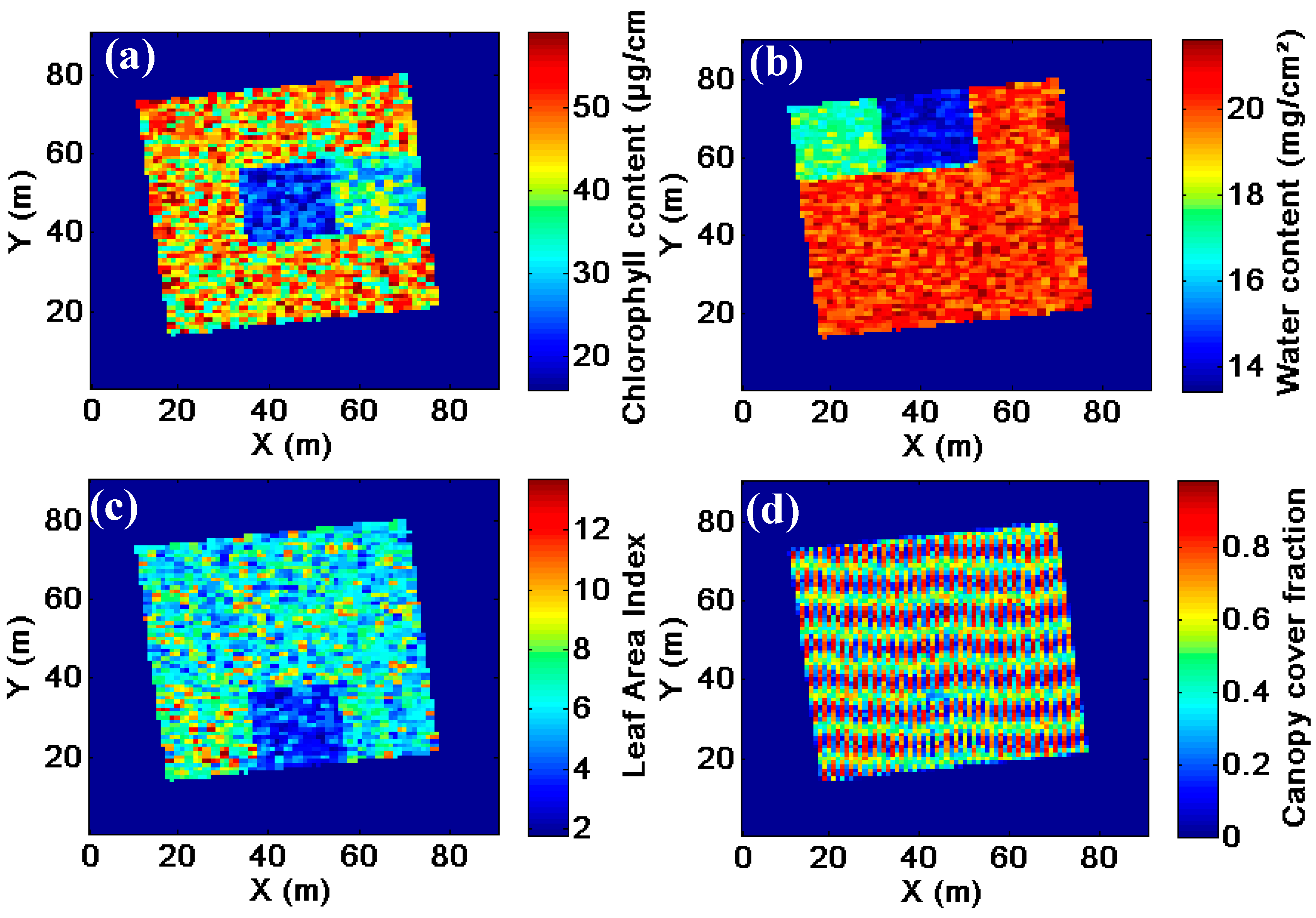
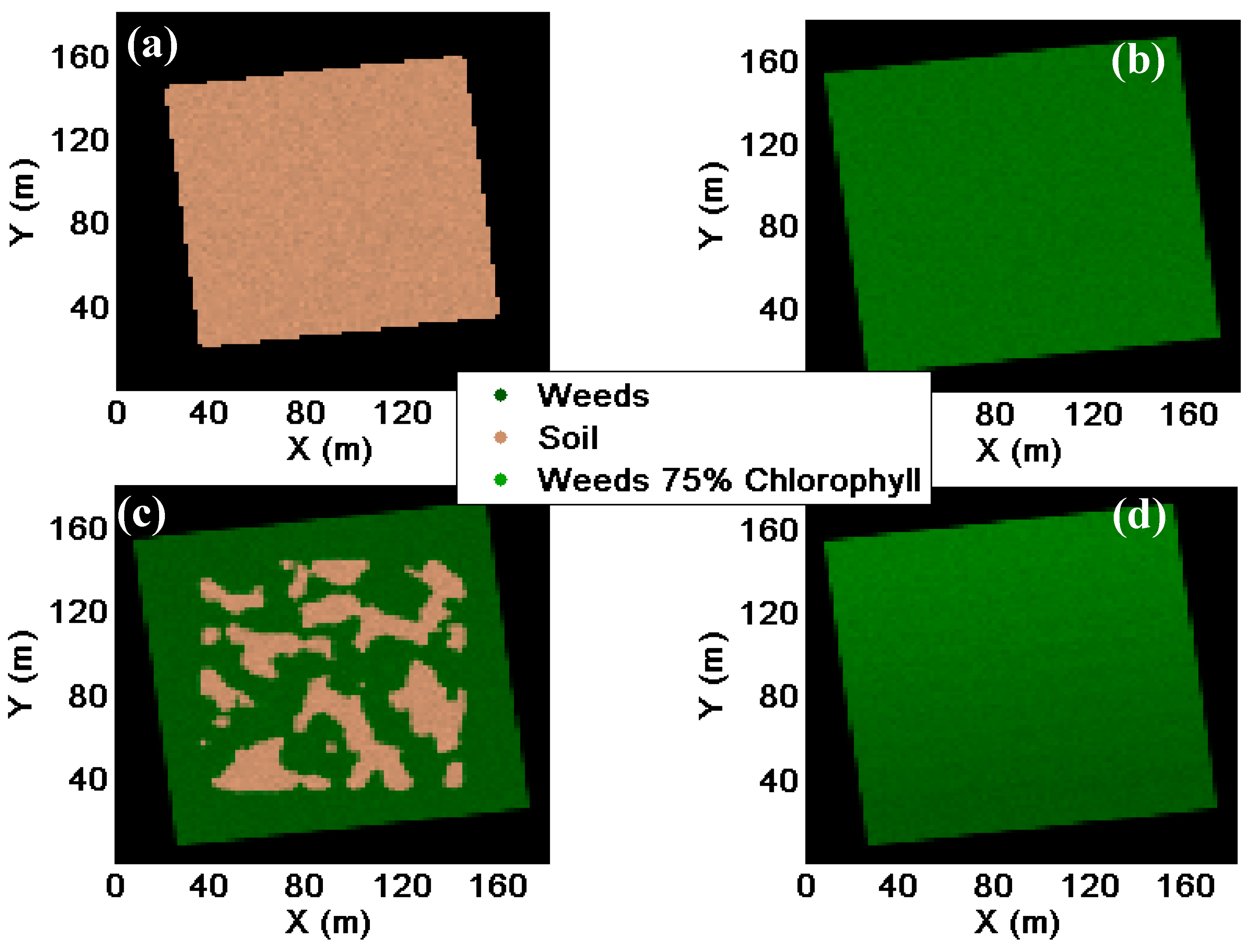
The goal of this study was to investigate the view-angle sensitivity of common spectral vegetation indices on the estimation of biophysical variables—i.e., chlorophyll content, water content and LAI—in orchards. In high spatial resolution imagery, changing view angles causes both BRDF- and mixture-related differences. As the latter influence can be minimized through a correction method, the view-angle sensitivity of common vegetation indices for high spatial resolution imagery of hedgerow cropping systems can be assessed and minimize the effects of varying viewing angles on change detection within and between time series. Synthetic imagery of a virtual orchard was used to include variable orchard conditions, as well as different background scenarios—i.e., non-vegetated, vegetated and partially vegetated. Finally, imagery from a satellite with off-nadir viewing capacities over an experimental orchard was investigated to highlight the importance of changing viewing geometry towards the estimation of biophysical variables.

2. Materials

2.1. Synthetic Imagery

Synthetic imagery was used in this study to improve our understanding of the effects of a changing viewing geometry on the remotely sensed data and the information derived from it [28,30,31]. The synthetic data provided exact cover fractions, spectral signatures and biophysical variables of the target crop for a range of viewing compositions. Additionally, the simulations were used to investigate the overall effect of viewing composition on the estimation of biophysical variables via vegetation indices.
In compliance with [28,31], the virtual orchard, developed by [32], consisted of virtual citrus trees (Citrus sinensis L.). The trees were arranged in a 3.5 by 2 m grid (row orientation of 7°; i.e., north-south direction). Within each orchard, several sections of the virtual orchard were modified to mimic stressed conditions for chlorophyll content, water content and LAI. Stressed leaf spectra were modified through PROSPECT [33]. Chlorophyll contents were extracted from in situ-measured unmodified leaf spectra and reduced by 25% and 50% and the water content by 15% and 30% [32]. LAI stress was introduced by randomly removing or adding leaves to the virtual trees representing 56% and 125% of the original LAI [32]. The spatial distribution and range of each variable is shown in Figure 1.
From these virtual orchards, different images were rendered in a physically-based ray-tracer (PBRT) [34]. The model has previously been calibrated and validated with the Radiation Transfer Model Intercomparison (RAMI) online model checker [35,36] and field data obtained in a citrus orchard in Wellington, South Africa [32,37]. Images were rendered with a direct and diffuse light source (solar elevation of 79.2° and solar azimuth of 339.6°) mimicking South African winter solstice [32]. The spectral range of the synthetic images was 350-2500 nm with a spectral resolution of 10 nm, while the spatial resolution of the sensor was fixed at 2 m. The resulting canopy cover fractions within the 2 m pixels are shown in Figure 1d. The influence of different viewing compositions was investigated by adjusting the position of the sensor. The sensor’s azimuth angles were varied between 0 and 315° with 45° increments and the sensor’s view angle was varied between 0 and 60° with 15° increments. As a result, each orchard composition was rendered from 33 different sensor positions.
The influence of different orchard conditions was investigated by varying the orchard floor or background through four different scenarios, while the position of the virtual trees remained identical for each scenario. Through these modifications, the sensitivity of commonly used vegetation indices to orchard- and viewing parameters could be investigated.
Scenario 1 (S1), a uniform soil background, consisting of an Albic Leptic Luvisol soil [38] measured in situ [39], shown in Figure 2a. Soil reflectance was assumed Lambertian.
Scenario 2 (S2), a uniform weed background (Figure 2b), consisting of Phleum pratense L. modeled with leaf reflectance obtained from the Leaf Optical Experiment database [32,40].
Scenario 3 (S3), a variable weed and soil background, consisting of a weed background with random and irregular soil patches (65/35% cover fraction distribution), depicted in Figure 2c.
Scenario 4 (S4), a variable weed background with a chlorophyll gradient. The weed background was modified similar to the leaf reflectances, increasing the chlorophyll content from 75% to the reference value (i.e., uniform weed background). A true color representation of the variable weed background is shown in Figure 2d.

2.2. Real Imagery

2.2.1. Study Area

The irrigated orchard, planted with Conference pear trees (Pyrus communis L. cv. “Conference”) on Quince C rootstock, was situated in Bierbeek, Belgium (50°49′34.59″N, 4°47′42.83″E). The 2.5 m high trees were planted in 2000 in a 3.5 by 1 meter grid. They were trained in a V-system with four fruiting branches on one central stem [41]. The orchard was situated on a south-east facing slope (3.5°) with a loamy soil and two dominant row azimuths, namely 41 and 131°. The trees received 100% of the crop evapotranspiration (ETc) [42,43], throughout most of the growing season.
The non-irrigated or rainfed orchard, situated in Kerkom, Belgium (50°46′24.25″N, 5°09′27.05″E), was planted in 2000 with Conference pear trees on Quince A rootstock. The 3.5 m high trees, planted in a 3.75 by 1.75 m grid, were trained in a Spindle bush system [41]. The orchard was situated on a south facing slope (1.1°) with a loamy soil and a row azimuth of 197°. The trees were rainfed and received no additional water input.
In both orchards, the soil under the trees was kept weed free for about 0.3 m from the trunk and grass was sown in between the tree rows.

2.2.2. Satellite Imagery

WorldView-2 multispectral images were acquired under different off-nadir viewing angles, with a ground sampling distance of 2.0 m and a spectral resolution complying eight bands: Coastal (400–450 nm), Blue (450–510 nm), Green (510–580 nm), Yellow (585–625 nm), Red (630–690 nm), Red Edge (705–745 nm), NIR1 (Near InfraRed 1; 770–895 nm) and NIR2 (860–1,040 nm). The acquisition details for the WorldView-2 images are shown in Table 1. All images were radiometrically [44], atmospherically [45] and geometrically corrected [46].

2.2.3. Reference Plots

During each satellite acquisition, ground reference plots were monitored, each plot consisting of four adjacent trees. In the rainfed orchard, 16 plots were selected on fixed intervals within two adjacent rows of similar structure and age. In the irrigated orchard, 32 plots were selected with variable age, soil type and row orientation. The position of each plot was determined with a differential global positioning system (Trimble RTK 58000). Spatial variation was introduced by the application of one-sided root-pruning (rainfed orchard) and deficit irrigation (irrigated orchard). The location of the ground measurements and both root-pruning and deficit irrigation treatments is shown in Figure 3.

3. Methods

3.1. Vegetation Indices

The spectral vegetation indices used in this study were divided into categories based on their proven or expected relationship with biophysical and structural variables (i.e., chlorophyll content, water content and LAI). The used vegetation indices are listed in Table 2 [5,8,9,47,48,49,50,51,52,53,54,55,56,57,58,59,60,61,62,63]. The indices were chosen because of a proven link with biophysical variables in fruit orchards [1,2,64].
Vegetation indices for which representative WorldView-2 band combinations were available, are also listed in Table 2. The conversion from narrowband to broadband vegetation indices should be viewed as an approximation as the exact wavelengths from the narrowband vegetation indices overlap in two or more satellite bands, e.g., WI (Water Index [9]).

3.2. Vegetation Index Correction

To remove canopy fraction differences for all high spatial resolution orchard images, a vegetation index correction was applied [28]. This correction algorithm rescaled the range of index values for all pixels to the range of index values for the pure canopy pixels (i.e., pixels with a canopy fractions over 0.8). The correction was applied in a moving window of size 7 by 7 pixels. Within each moving window, (i) background was assumed uniform, (ii) the pure canopy pixels were assumed to represent the true vegetation index range in the pure canopy pixels for that moving window and (iii) the presence of the full range of canopy fractions was assumed. Before the correction was applied, outliers were detected and removed, based on the threshold of 1.5 times the inter-quartile range from the upper or lower quartile [65]. Afterwards, the index values for each pixel were averaged from all the moving windows that included that pixel. In general, this correction assumed that the variability along the y-axis (i.e., vegetation index value) was only caused by the variability in tree conditions, while the variability along the x-axis (i.e., canopy fraction) was caused by the admixture of the background component. More information on this vegetation index correction can be found in [28].
For the synthetic images, the exact tree cover was known for each pixel. For the real satellite imagery, the canopy cover fraction was estimated through a Gram-Schmidt pan-sharpening [66] to produce multispectral bands with a panchromatic resolution (0.5 m). This pan-sharpened image was classified through unsupervised classification [67] and resampled for each 2 m multispectral pixel to provide an estimation of the canopy fractions, similar to Hamada et al. [68].

3.3. Determination of in situ Measured Biophysical and Structural Variables

During satellite acquisitions, biophysical variables were determined based on the inversion of leaf spectral measurements on 20 samples per plot. A validation experiment was acquired with lab measured chlorophyll and water content which achieved R2 values of 0.79 and 0.85 between measured and modeled water and chlorophyll content respectively (results not shown here). In addition, hemispherical photographs were collected for each plot using a Kodak Professional DCS 660 digital camera (6 mega pixels) with a Sigma 8mm Circular Fisheye lens (Sigma Corporation, Tokyo, Japan). Each plot was sampled 5 times at fixed positions [69] and processed with the CAN-EYE software to determine LAI based on canopy gap fraction [70]. An overview of the mean and standard deviations of for both orchards is shown in Table 3.

4. Results

4.1. Synthetic Imagery

The synthetic imagery in this study provided exact cover fractions, spectral signatures and biophysical variables of the target crop for a range of view angles. The simulations were used to investigate the overall effect of viewing geometry on the estimation of biophysical variables through vegetation indices without the influence of sensor/target anomalies.
In a first step the ground references or tree endmembers—pure canopy pixels collected from scenes of individual trees without background—were used to illustrate optimal coefficient of determination values (R2) between biophysical variables and vegetation indices. The variation of R2 values between vegetation indices and chlorophyll content, water content and LAI for different viewing compositions is shown in Figure 4. As only pure canopy pixels were used, view angle effects regarding variable canopy fraction distributions could be assumed absent and resulting effects attributed to BRDF.
Figure 4 illustrates the complexity of viewing composition influences on biophysical and structural variables estimation through vegetation indices. On the one hand, several indices—such as the NDVI, TCARI, PRI and CAI indices—showed an increase of R2 values with increased sensor zenith angles. On the other hand, the sLAIDI showed higher R2 values with LAI at nadir compared to off-nadir viewing angles. Figure 4 was only illustrative for imagery under ideal circumstances—i.e., pure canopy scenes without the influence of background. Therefore, the viewing composition distribution of R2 values for the uniform weed background (S2) are shown in Figure 5 prior to the vegetation index correction (Section 3.2). Figure 5 was limited to results from the S2 background scenario, as other scenarios presented similar distributions.
The distribution of R2 values in Figure 5 illustrated the influence of variable viewing angles on vegetation indices in a realistic scenario (i.e., uniform background of vegetation). For several indices, this distribution was mirrored around the row orientation (i.e., NDVI, SRPI, PRI, SIPI and NDII). This effect could most likely be attributed to variable canopy fraction distribution, as off-nadir viewing imagery perpendicular to the row orientation would represent a decreasingly smaller fraction of background. To circumvent this problem, a vegetation index correction algorithm (Section 3.2) was applied. The distribution of R2 values for S2 after the correction is shown in Figure 6. In addition, viewing geometry differences for R2 values between index values and biophysical variables are listed in Table 4. For Table 4, the differences between viewing compositions were quantified through the range of R2 values for each index and all viewing compositions in each scenario (Section 2.1).
Despite the correction algorithm removing the effects of variable canopy distribution in Figure 6 and Table 4, several indices were still significantly dependent on viewing composition. Only the distribution of R2 values for S2 was shown in Figure 6, as other background scenarios showed similar distributions, although the scale varied depending on either vegetated or non-vegetated background scenarios.
Figure 6 shows the dependency of viewing compositions for several vegetation indices while estimating biophysical and structural variables. Some indices showed higher R2 values for nadir viewing scenes and a decrease towards more off-nadir viewing scenes, for example the ZM (Figure 6e), SIPI (Figure 6k) and GM1 indices (Figure 6l). SRPI (Figure 6f), PRI (Figure 6g) and NDII (Figure 6s) showed increased R2 values for off-nadir scenes perpendicular to the row orientation, while R2 values decreased for scenes parallel to row orientation for higher sensor zenith angles.

4.2. Real Imagery

Similarly to the synthetic imagery, the satellite imagery was corrected for canopy cover fraction distribution based on the vegetation index correction algorithm described in [28]. Afterwards, index values for each plot were extracted. The R2 values between vegetation indices and measured biophysical variables are presented in Table 5.
The results depicted in Table 5 showed significant correlations between biophysical variables and vegetation indices when combining both orchards. Significant R2 values were found between chlorophyll content and the PRI, SRPI, NPCI and CTR1 indices. However, after processing imagery for both orchards separately, significantly higher R2 values were found in the rainfed orchard for chlorophyll related indices. For example, R2 values of 0.64, 0.59 and 0.58 for OSAVI, NDVI and CTR2 index values respectively. On the other hand, indices in the irrigated orchard showed no significant correlations. To visualize the influence of variable viewing geometry on the relationship between index values and biophysical variables, R2 values were calculated for each available viewing composition. In order to compare different row orientations, only the relative angle between the row azimuth and view azimuth was used. The results are shown in Figure 7.
Figure 7 showed the influence of viewing geometry on the estimation of biophysical and structural variables through vegetation indices. For several indices, the shaded side of the canopy presented higher R2 values compared to the sunlit side—i.e., NDVI (Figure 7a), MCARI (Figure 7c), TCARI (Figure 7d), CTR2 (Figure 7j) and RDVI (Figure 7q). Conversely, several indices were presenting higher R2 values for the sunlit side compared to the shaded side—i.e., CTR1 (Figure 7i) and TVI (Figure 7r). Finally, some indices presented high R2 values for both sunlit and shaded sides—i.e., OSAVI (Figure 7b), SIPI (Figure 7k) and WI (Figure 7m)—further illustrating that variable viewing geometry should be avoided or accounted for.

5. Discussion

The use of remote sensing within capital intensive orchard crops provides alternatives to time consuming, labor intensive and destructive in situ measurements. Practical use in hedgerow orchards under temperate climate conditions requires the use of high spatial resolution satellite sensors with off-nadir viewing capabilities [10,11]. However, this presence of variable viewing angles could affect the relationship between biophysical variables and spectral measurements [4,12,13]. Moreover, variable viewing angles within and between time series could obstruct the distinction between genuine changes and viewing geometry influences. In this study, the distribution of R2 values for different viewing compositions (Figure 4, Figure 5, Figure 6 and Figure 7) and the ranges for different background scenarios (Table 4) showed the necessity of careful selection of vegetation indices for applications using spectral imagery acquired under or subject to multiple viewing geometries.
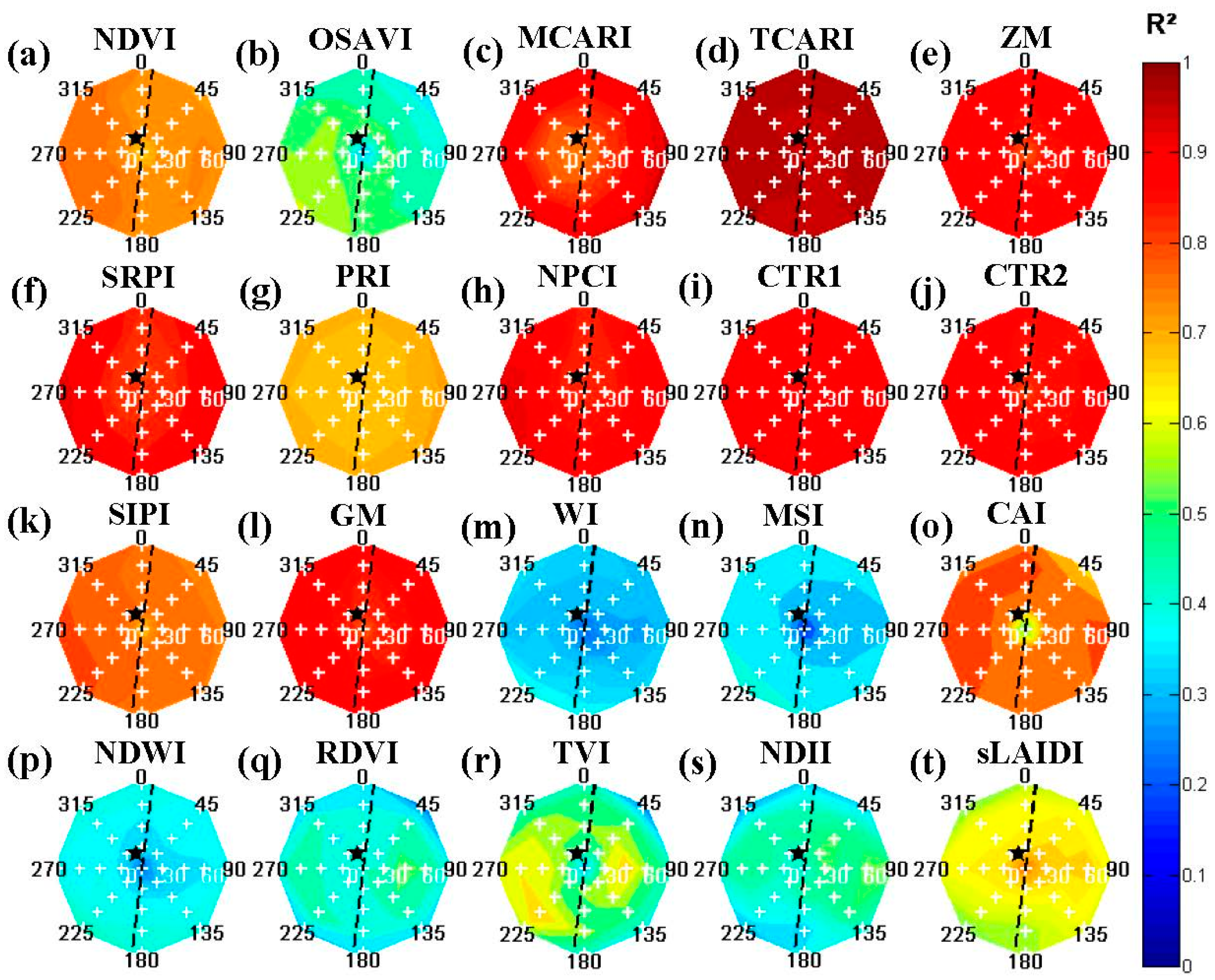
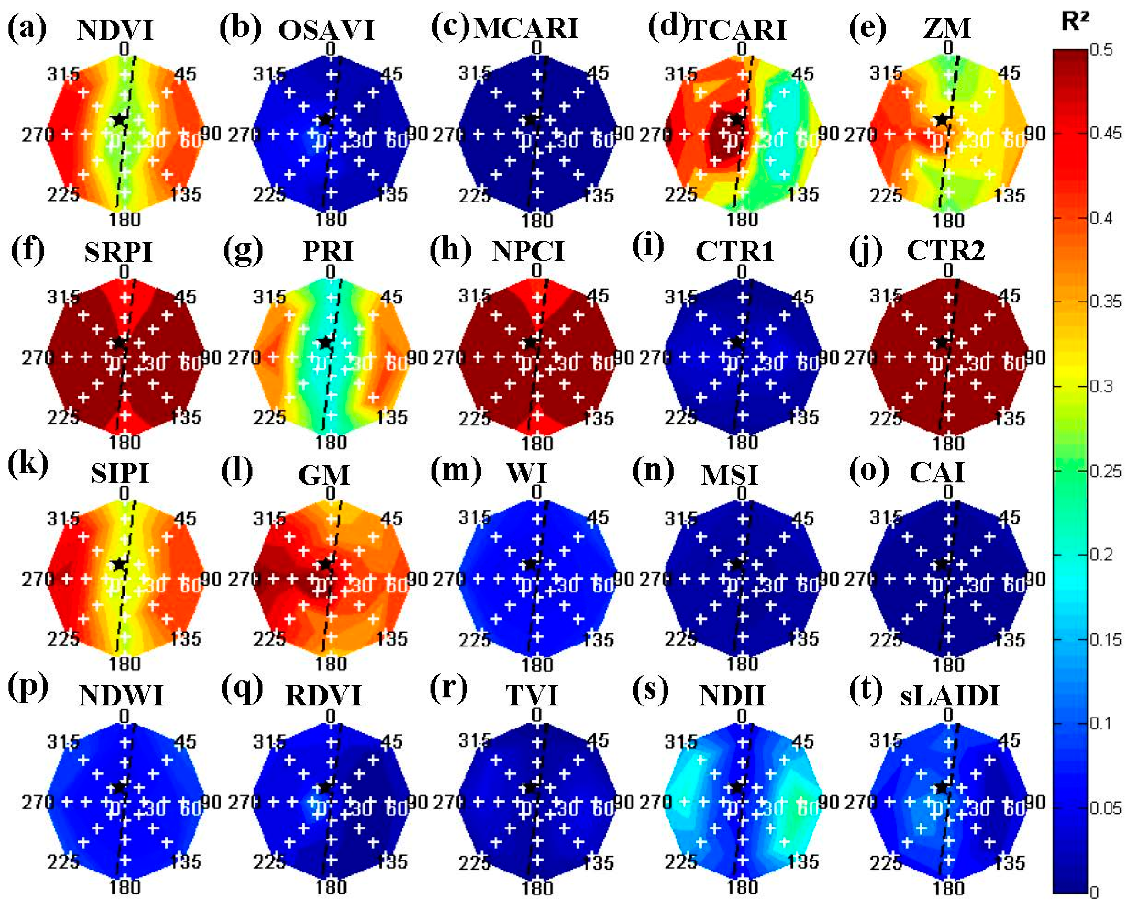
For high spatial resolution imagery, changing viewing geometries would cause both differences related to Bidirectional Reflectance Distribution Function (BRDF) influences [21] and to variable canopy fraction mixtures. The former was visible for the tree endmembers, rendered without background and extracted from pure canopy pixels (Figure 4). For these reference images, several indices showed a variable distribution favoring more nadir viewing—i.e., sLAIDI (Figure 4t)—or off-nadir viewing scenes—i.e., OSAVI (Figure 4b), WI (Figure 4m), CAI (Figure 4o) and TVI (Figure 4r). These effect could be attributed to the inherent BRDF effects and should be avoided or corrected for [16,17,18,19,20,21]. However, other indices showed a less significant change in R2 values and were less affected for these ideal circumstances.
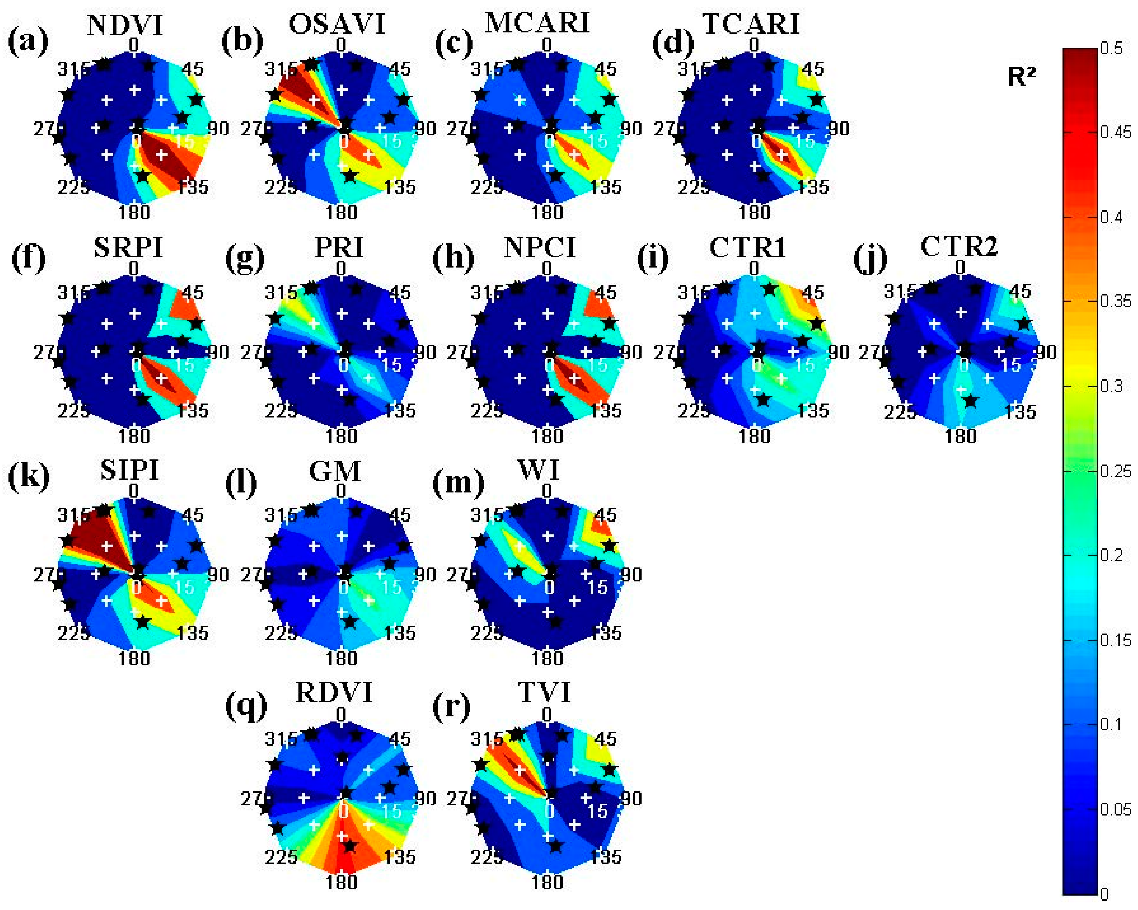
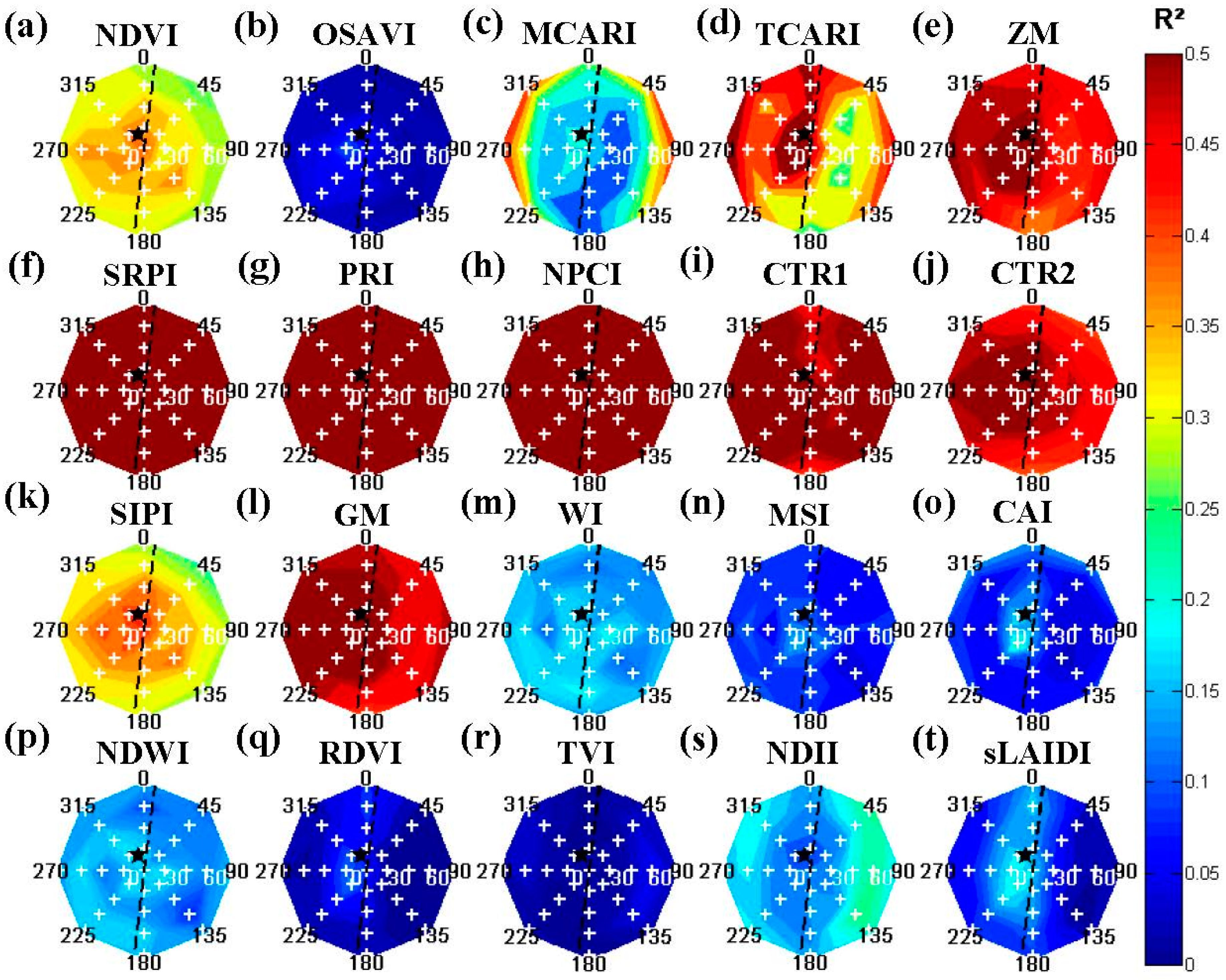
The synthetic imagery also demonstrated a high dependence of several indices towards canopy fraction distribution (Figure 5), which was removed through a vegetation index correction (Figure 6). After the correction, the lowest R2 values from the synthetic imagery were found for the most variable background scenario—i.e., the soil and weed background or S3 (Table 4). Generally, the differences between different background scenarios were relatively small. This was most likely the result of the vegetation index correction [28], which removed most of the influence of background mixtures and variable canopy cover fractions. Exceptions hereof were indices that were related to vegetative cover fraction, e.g., NDVI [71], which showed significantly higher R2 values for vegetated backgrounds (S2 and S4, Table 4) compared to non-vegetated backgrounds (S1 and S3, Table 4). This could be the result of the assumption of Lambertian behavior for the soil backgrounds. Although the range of R2 values will be similar, the R2 values could be lower for non-Lambertian backgrounds. Overall, the R2 values were significantly higher between vegetation indices and chlorophyll content compared to LAI and water content, because of larger differences between treatments and the inherent relationship between leaf area and the amount of canopy water content [5].
For the synthetic imagery, several commonly used vegetation indices presented an influence towards variable viewing geometries. PRI, NDII and SRPI values showed higher R2 values perpendicular to the row orientation compared to parallel to rows for higher off-nadir view angles (Figure 6). This might be attributed to the inclusion of background with parallel viewing to the rows, as imagery perpendicular to the rows would not present any background. Overall, differences between off-nadir viewing parallel or perpendicular to the row orientation might be greater without the use of the vegetation index correction to normalize for different canopy cover fractions. On the other hand, this view angle sensitivity of PRI was similar to [24,25,72], finding a large difference between PRI values from forward (shaded) and backward (sunlit) scattered scenes. Other indices, such as NDVI, GM, ZM and SIPI, showed a decrease in R2 values from nadir to off-nadir viewing scenes (Figure 6). These results were similar to studies indicating a high dependence of NDVI towards variable viewing angles [24,73,74] and a degraded correlation with NDVI-derived products [18].
The R2 values of satellite derived vegetation indices (Table 5) were significantly lower compared to the synthetic images (Table 4). This was most likely by the restricted amount of point measurements for the real imagery and the use of different row orientations within and between the orchards. On the other hand, also a suboptimal vegetation index correction could cause a decrease in R
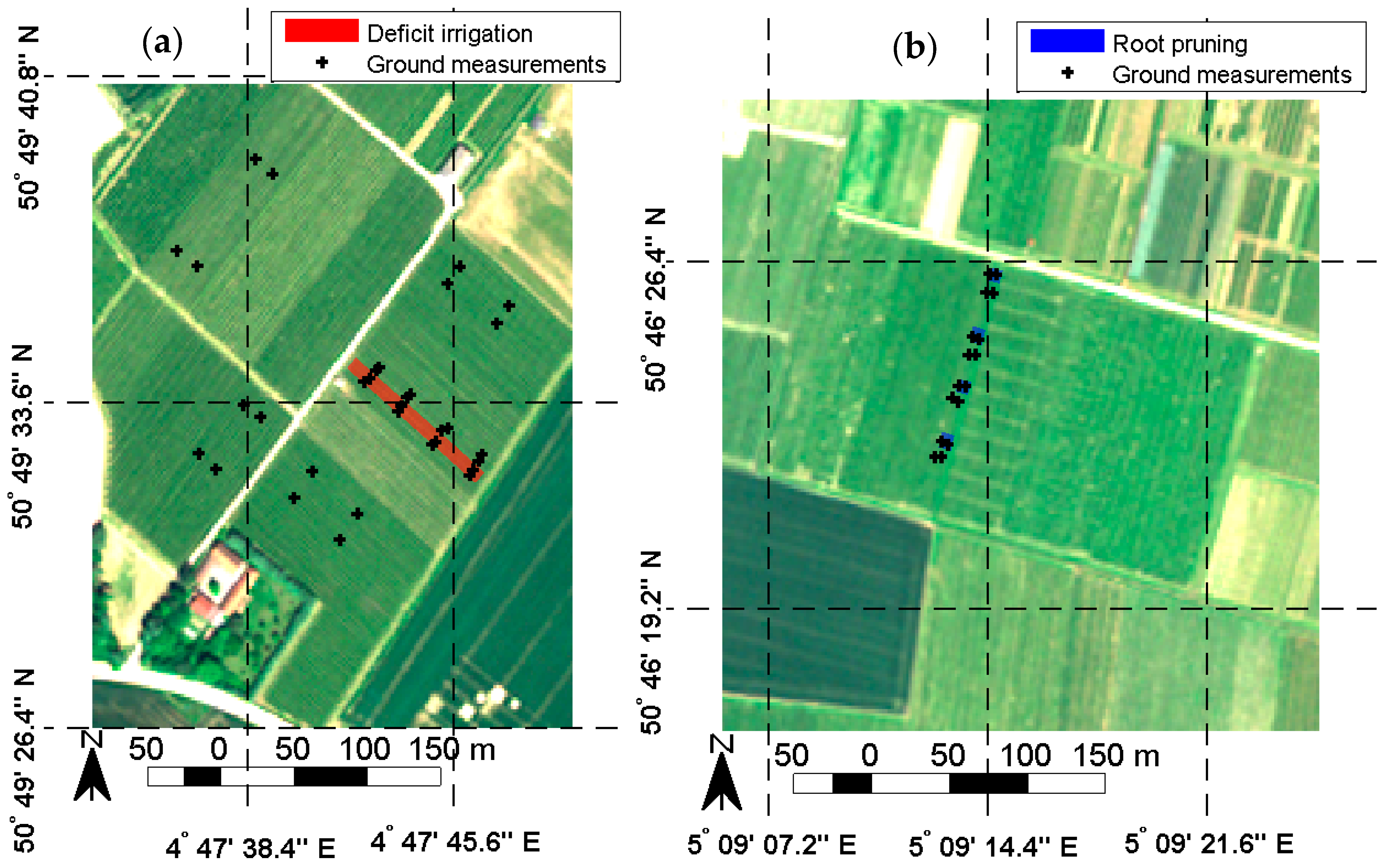
2 values between indices and variables. For the rainfed orchard, R2 increased significantly because of the similar row azimuth for all ground control plots. For the irrigated orchard, a significant decrease in R2 values was the result of both sunlit and shaded canopies within one scene, as both 41 and 131° row orientations were monitored. The increased influence of shadow compared to the synthetic imagery was caused by a decrease in illumination elevation and the presence of a hedgerow cropping system causing one predominantly shaded and sunlit side [41,75]. Several studies have shown the negative effect of shaded canopy parts on the correlation between vegetation indices and biophysical variables [3,4,76]. As the virtual orchard trees consisted of spherical canopies, shaded canopy sections and the effects of shadow on the vegetation indices were of less importance [3].
The vegetation index correction algorithm could not mitigate the inclusion of shadow on the variation of index values, as it is not directly related to canopy cover fraction. Conversely, problems could be avoided by segmenting or classifying the canopies into sunlit and shaded areas—e.g., Stagakis et al. [2,3]. However, for hedgerow systems problems with canopy anisotropy would be enlarged and cause significant differences between both faces of the canopy [13], obstructing derivation of structural variables—i.e., plant cover, canopy height and biomass—from multiple viewing angles. Another solution would be the minimization of shaded pixels in the analysis [3,76,77]. To illustrate the usefulness of this approach, a selection was made for all satellite images (Section 2.2) based on row orientation, viewing and illumination angles. Similarly to [4], scenes with high off-nadir viewing angles—i.e., off-nadir viewing angles over 20°—and viewing geometries opposite to the sun were removed as they consisted mostly of shaded canopies. Off-nadir viewing angles under 20° would result in partially sunlit scenes and were shown less affected [4]. The average R2 values for all indices after the selection of sunlit image pixels are shown in Table 6.
Table 6 illustrated the usefulness of pixel selection based on scene illumination for the irrigated orchard, as a significant increase in R2 values was found between biophysical variables and index values compared to Table 5. The indices showing a significant increase also showed higher R2 values for sunlit scene compositions in Figure 7. On the other hand, indices which presented higher R2 values for shaded scene compositions—i.e., NDVI, CTR2, MCARI, OSAVI and TCARI—showed similar or decreased R2 values.
For the rainfed orchard, a significant decrease of R2 values was present for almost all indices after the selection of sunlit pixels compared to Table 5. This was the effect of the different growing systems within both orchards. On the one hand, the Spindle bush system (rainfed orchard) resulted in open tree canopies and more sunlit areas [41]. On the other hand, the hedgerow V-system (irrigated orchard) resulted in variable canopy faces—i.e., one predominantly sunlit and shaded side [41].
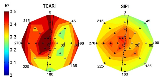
With regards to the optimal vegetation indices for high spatial resolution imagery, PRI, CTR1, SIPI and GM provided more stable correlations with chlorophyll content for variable viewing geometries (Figure 6, Table 5 and Table 6). However, these indices were highly affected by the canopy fraction distribution and should be corrected or normalized prior to analysis (Figure 5 and Figure 6). With regards to water content and LAI, WI and sLAIDI provided good correlations for nadir viewing scenes, with a significant decrease towards off-nadir viewing angles. Other vegetation indices could be used in certain circumstances, but should be avoided in time series with variable viewing angles, e.g., NDVI, OSAVI, MCARI, TCARI, RDVI and TVI (Figure 6, Table 5 and Table 6). Although the vegetation indices (Table 2) were selected based on previous studies in fruit orchards, the list was not complete [1,2,64]. Further research is required for vegetation indices not represented here prior to their use for applications with multiple viewing angles.
Overall, the results illustrated the necessity of a vegetation index selection or correction based on each specific circumstance and data set. However, through the careful selection of vegetation indices, an optimal derivation of biophysical variable should be plausible for applications with multiple viewing angles. Moreover, depending on the size of the available time series for a fixed target location, index values could be normalized with regards to view angle—e.g., Seaquist and Olsson [73]. However, the most important limitation to this approach is the high amount of images required within a relatively small time window to minimize influences of a changing solar angle.

6. Conclusions

Stress-related biophysical and structural variables of capital intensive orchard crops can be approximated with accurate and consistent estimations of spectral vegetation indices from off-nadir viewing satellite imagery. However, the variable viewing compositions of each image could affect this relationship. Most of the research studying this effect has focused on cropping systems with complete canopy cover, while imagery over orchard cropping systems could cause mixtures between canopies and backgrounds. This study investigated the sensitivity of common spectral vegetation indices on changing viewing geometries and its relationship with the estimation of biophysical variables—i.e., chlorophyll content, water content and Leaf Area Index (LAI). Ultimately to minimize variable viewing influences within and between time series, which could obstruct change detection because of the confusion with genuine changes. This was achieved through the use of synthetic and satellite imagery over a virtual citrus orchard and an experimental hedgerow pear orchard respectively.
Results indicated significant differences between nadir and off-nadir viewing scenes for some indices (∆R2 > 0.4). Several indices—such as the Photochemical Reflectance Index (PRI), Normalized Difference Infrared Index (NDII) and Simple Ratio Pigment Index (SRPI)—showed higher coefficient of determination (R2) values for higher off-nadir view angles perpendicular compared to parallel to the row orientation. On the other hand, indices—such as the Normalized Difference Vegetation Index (NDVI), Gitelson and Merzlyak (GM), Zarco and Miller (ZM) and Structure Insensitive Pigment Index (SIPI)—showed a decrease in R2 values from nadir to off-nadir viewing scenes.
In general, this study showed the necessity for a careful selection of vegetation indices for estimating biophysical variables, especially for applications with multiple viewing angles.

Acknowledgments

This work was supported by the Agency for Innovation by Science and Technology in Flanders (IWT-Vlaanderen). The research was funded through a project in cooperation with the Soil Service of Belgium (BDB) and the Research Center for Fruit (Proefcentrum Fruitteelt in Sint-Truiden). The authors would like to thank fruit grower Jan Vandervelpen for allowing research in his orchard and making this work possible.

Author Contributions

The contribution of the authors to this work were: Jonathan Van Beek 1,2,3,4,5, Laurent Tits 2,3,4, Ben Somers 2,3,4, Tom Deckers 1,4,5, Pieter Janssens 1,4,5 and Pol Coppin 1,4,5. 1 Experimental design; 2 analysis and interpretation; 3 manuscript preparation and writing; 4 paper review; 5 project coordination.

Conflicts of Interest

The authors declare no conflict of interest.

References

  1. Zarco-Tejada, P.J.; Berjon, A.; Lopez-Lozano, R.; Miller, J.R.; Martin, P.; Cachorro, V.; Gonzalez, M.R.; de Frutos, A. Assessing vineyard condition with hyperspectral indices: Leaf and canopy reflectance simulation in a row-structured discontinuous canopy. Remote Sens. Environ. 2005, 99, 271–287. [Google Scholar] [CrossRef]
  2. Stagakis, S.; Markos, N.; Sykioti, O.; Kyparissis, A. Monitoring canopy biophysical and biochemical parameters in ecosystem scale using satellite hyperspectral imagery: An application on a Phlomis fruticosa Mediterranean ecosystem using multiangular CHRIS/PROBA observations. Remote Sens. Environ. 2010, 114, 977–994. [Google Scholar] [CrossRef]
  3. Stagakis, S.; González-Dugo, V.; Cid, P.; Guillén-Climent, M.L.; Zarco-Tejada, P.J. Monitoring water stress and fruit quality in an orange orchard under regulated deficit irrigation using narrow-band structural and physiological remote sensing indices. ISPRS J. Photogramm. Remote Sens. 2012, 71, 47–61. [Google Scholar] [CrossRef]
  4. Van Beek, J.; Tits, L.; Somers, B.; Coppin, P. Stem Water Potential Monitoring in Pear Orchards through WorldView-2 Multispectral Imagery. Remote Sens. 2013, 5, 6647–6666. [Google Scholar] [CrossRef]
  5. Delalieux, S.; Somers, B.; Hereijgers, S.; Verstraeten, W.; Keulemans, W.; Coppin, P. A near-infrared narrow-waveband ratio to determine Leaf Area Index in orchards. Remote Sens. Environ. 2008, 112, 3762–3772. [Google Scholar] [CrossRef]
  6. Pinter, P.J.; Hatfield, J.L.; Schepers, J.S.; Barnes, E.M.; Moran, M.S.; Daughtry, C.S.T.; Upchurch, D.R. Remote Sensing for Crop Management. Photogramm. Eng. Remote Sens. 2003, 69, 647–664. [Google Scholar] [CrossRef]
  7. Dorigo, W.A.; Zurita-Milla, R.; de Wit, A.J.W.; Brazile, J.; Singh, R.; Schaepman, M.E. A review on reflective remote sensing and data assimilation techniques for enhanced agroecosystem modeling. Int. J. Appl. Earth Obs. Geoinf. 2007, 9, 165–193. [Google Scholar] [CrossRef]
  8. Gamon, J.A.; Penuelas, J.; Field, C.B. A narrow-waveband spectral index that tracks diurnal changes in photosynthetic efficiency. Remote Sens. Environ. 1992, 41, 35–44. [Google Scholar]
  9. Penuelas, J.; Filella, I.; Biel, C.; Serrano, L.; Savé, R. The reflectance at the 950–970 nm region as an indicator of plant water status. Int. J. Remote Sens. 1993, 14, 1887–1905. [Google Scholar] [CrossRef]
  10. Moran, S.; Fitzgerald, G.; Rango, A.; Walthall, C.; Barnes, E.; Bausch, W.; Clarke, T.; Daughtry, C.; Everitt, J.; Escobar, D.; et al. Sensor Development and Radiometric Correction for Agricultural Applications. Photogramm. Eng. Remote Sens. 2003, 69, 705–718. [Google Scholar] [CrossRef]
  11. Perry, E.M.; Dezzani, R.J.; Seavert, C.F.; Pierce, F.J. Spatial variation in tree characteristics and yield in a pear orchard. Precis. Agric. 2009, 11, 42–60. [Google Scholar] [CrossRef]
  12. Stuckens, J.; Dzikiti, S.; Verstraeten, W.W.; Verreynne, S.; Swennen, R.; Coppin, P. Physiological interpretation of a hyperspectral time series in a citrus orchard. Agric. For. Meteorol. 2011, 151, 1002–1015. [Google Scholar] [CrossRef]
  13. Meggio, F.; Zarco-Tejada, P.J.; Miller, J.R.; Martín, P.; González, M.R.; Berjón, A. Row orientation and viewing geometry effects on row-structured vine crops for chlorophyll content estimation. Can. J. Remote Sens. 2008, 34, 220–234. [Google Scholar]
  14. Chopping, M.; Moisen, G.G.; Su, L.; Laliberte, A.; Rango, A.; Martonchik, J.V.; Peters, D.P.C. Large area mapping of southwestern forest crown cover, canopy height, and biomass using the NASA Multiangle Imaging Spectro-Radiometer. Remote Sens. Environ. 2008, 112, 2051–2063. [Google Scholar] [CrossRef]
  15. Wolf, A.; Berry, J.A.; Asner, G.P. Allometric constraints on sources of variability in multi-angle reflectance measurements. Remote Sens. Environ. 2010, 114, 1205–1219. [Google Scholar] [CrossRef]
  16. Shepherd, J.D.; Dymond, J.R. BRDF Correction of Vegetation in AVHRR Imagery. Remote Sens. Environ. 2000, 74, 397–408. [Google Scholar] [CrossRef]
  17. Schaaf, C.B.; Gao, F.; Strahler, A.H.; Lucht, W.; Li, X.; Tsang, T.; Strugnell, N.C.; Zhang, X.; Jin, Y.; Muller, J.-P.; et al. First operational BRDF, albedo nadir reflectance products from MODIS. Remote Sens. Environ. 2002, 83, 135–148. [Google Scholar] [CrossRef]
  18. Huete, A.; Didan, K.; Miura, T.; Rodriguez, E.; Gao, X.; Ferreira, L. Overview of the radiometric and biophysical performance of the MODIS vegetation indices. Remote Sens. Environ. 2002, 83, 195–213. [Google Scholar] [CrossRef]
  19. Vermote, E.; Justice, C.O.; Breon, F.-M. Towards a Generalized Approach for Correction of the BRDF Effect in MODIS Directional Reflectances. IEEE Trans. Geosci. Remote Sens. 2009, 47, 898–908. [Google Scholar] [CrossRef]
  20. Bréon, F.-M.; Vermote, E. Correction of MODIS surface reflectance time series for BRDF effects. Remote Sens. Environ. 2012, 125, 1–9. [Google Scholar] [CrossRef]
  21. De Abelleyra, D.; Verón, S.R. Comparison of different BRDF correction methods to generate daily normalized MODIS 250m time series. Remote Sens. Environ. 2014, 140, 46–59. [Google Scholar] [CrossRef]
  22. Sandmeier, S.; Müller, C.; Hosgood, B.; Andreoli, G. Physical mechanisms in hyperspectral BRDF data of grass and watercress. Remote Sens. Environ. 1998, 66, 222–233. [Google Scholar] [CrossRef]
  23. Okin, G.S.; Clarke, K.D.; Lewis, M.M. Comparison of methods for estimation of absolute vegetation and soil fractional cover using MODIS normalized BRDF-adjusted reflectance data. Remote Sens. Environ. 2013, 130, 266–279. [Google Scholar] [CrossRef]
  24. Verrelst, J.; Schaepman, M.E.; Koetz, B.; Kneubühler, M. Angular sensitivity analysis of vegetation indices derived from CHRIS/PROBA data. Remote Sens. Environ. 2008, 112, 2341–2353. [Google Scholar] [CrossRef]
  25. Hall, F.G.; Hilker, T.; Coops, N.C.; Lyapustin, A.; Huemmrich, K.F.; Middleton, E.; Margolis, H.; Drolet, G.; Black, T.A. Multi-angle remote sensing of forest light use efficiency by observing PRI variation with canopy shadow fraction. Remote Sens. Environ. 2008, 112, 3201–3211. [Google Scholar] [CrossRef]
  26. Galvão, L.S.; Roberts, D.A.; Formaggio, A.R.; Numata, I.; Breunig, F.M. View angle effects on the discrimination of soybean varieties and on the relationships between vegetation indices and yield using off-nadir Hyperion data. Remote Sens. Environ. 2009, 113, 846–856. [Google Scholar] [CrossRef]
  27. Stuckens, J.; Somers, B.; Albrigo, G.L.; Dzikiti, S.; Verstraeten, W.W. Off-nadir Viewing for Reducing Spectral Mixture Issues in Citrus Orchards. Photogramm. Eng. Remote Sens. 2010, 76, 1261–1274. [Google Scholar] [CrossRef]
  28. Van Beek, J.; Tits, L.; Somers, B.; Deckers, T.; Janssens, P.; Coppin, P. Reducing background effects in orchards through spectral vegetation index correction. Int. J. Appl. Earth Obs. Geoinf. 2014, 34, 167–177. [Google Scholar] [CrossRef]
  29. Tits, L.; Somers, B.; Saeys, W.; Coppin, P. Site-Specific Plant Condition Monitoring through Hyperspectral Alternating Least Squares Unmixing. IEEE J. Sel. Top. Appl. Earth Obs. Remote Sens. 2014, 7, 3606–3618. [Google Scholar] [CrossRef]
  30. Tits, L.; De Keersmaecker, W.; Somers, B.; Asner, G.P.; Farifteh, J.; Coppin, P. Hyperspectral shape-based unmixing to improve intra- and interclass variability for forest and agro-ecosystem monitoring. ISPRS J. Photogramm. Remote Sens. 2012, 74, 163–174. [Google Scholar] [CrossRef]
  31. Tits, L.; Somers, B.; Stuckens, J.; Farifteh, J.; Coppin, P. Integration of in situ measured soil status and remotely sensed hyperspectral data to improve plant production system monitoring: Concept, perspectives and limitations. Remote Sens. Environ. 2013, 128, 197–211. [Google Scholar] [CrossRef]
  32. Stuckens, J.; Somers, B.; Delalieux, S.; Verstraeten, W.W.; Coppin, P. The impact of common assumptions on canopy radiative transfer simulations: A case study in Citrus orchards. J. Quant. Spectrosc. Radiat. Transf. 2009, 110, 1–21. [Google Scholar] [CrossRef]
  33. Jacquemoud, S.; Baret, F. Prospect: A model of leaf optical properties spectra. Remote Sens. Environ. 1990, 34, 75–91. [Google Scholar] [CrossRef]
  34. Pharr, M.; Humphreys, G. Physically Based Rendering, From Theory to Implementation; Morgan Kaufmann: San Fransisco, CA, USA, 2004; p. 1019. [Google Scholar]
  35. Widlowski, J.-L.; Taberner, M.; Pinty, B.; Bruniquel-Pinel, V.; Disney, M.; Fernandes, R.; Gastellu-Etchegorry, J.-P.; Gobron, N.; Kuusk, A.; Lavergne, T.; et al. Third Radiation Transfer Model Intercomparison (RAMI) exercise: Documenting progress in canopy reflectance models. J. Geophys. Res. 2007, 112, D09111. [Google Scholar] [CrossRef]
  36. Widlowski, J.-L.; Mio, C.; Disney, M.; Adams, J.; Andredakis, I.; Atzberger, C.; Brennan, J.; Busetto, L.; Chelle, M.; Ceccherini, G.; et al. The fourth phase of the radiative transfer model intercomparison (RAMI) exercise: Actual canopy scenarios and conformity testing. Remote Sens. Environ. 2015, 169, 418–437. [Google Scholar] [CrossRef]
  37. Somers, B.; Delalieux, S.; Verstraeten, W.W.; Coppin, P. A Conceptual Framework for the Simultaneous Extraction of Sub-pixel Spatial Extent and Spectral Characteristics of Crops. Photogramm. Eng. Remote Sens. 2009, 75, 57–68. [Google Scholar] [CrossRef]
  38. FAO. Soils Map of the World: Revised Legend; Food and Agriculture Organization of the United Nations: Rome, Italy, 1988. [Google Scholar]
  39. Somers, B.; Gysels, V.; Verstraeten, W.W.; Delalieux, S.; Coppin, P. Modelling moisture-induced soil reflectance changes in cultivated sandy soils: a case study in citrus orchards. Eur. J. Soil Sci. 2010, 61, 1091–1105. [Google Scholar] [CrossRef]
  40. Hosgood, B.; Jacquemoud, S.; Andreoli, G.; Verdebout, J.; Pedrini, A.; Schmuck, G. Leaf Optical Properties EXperiment 93 (LOPEX93); Report EUR 16095 EN; European Commission—Joint Research Centre: Ispra, Italy, 1994. [Google Scholar]
  41. Sansavini, S.; Musacchi, S. Canopy architecture, training and pruning in the modern European pear orchards: An overview. Acta Hortic. 1994, 367, 152–172. [Google Scholar] [CrossRef]
  42. Allen, R.G.; Pereira, L.S.; Raes, D.; Smith, M. Crop Evapotranspiration—Guidelines for Computing Crop Water Requirements—FAO Irrigation and Drainage Paper 56; FAO: Rome, Italy, 1998. [Google Scholar]
  43. Janssens, P.; Deckers, T.; Elsen, F.; Elsen, A.; Schoofs, H.; Verjans, W.; Vandendriessche, H. Sensitivity of root pruned “Conference” pear to water deficit in a temperate climate. Agric. Water Manag. 2011, 99, 58–66. [Google Scholar] [CrossRef]
  44. Updike, T.; Comp, C. Radiometric Use of WorldView-2 Imagery Technical Note; DigitalGlobe: Westminster, CO, USA, 2010; p. 16. [Google Scholar]
  45. Adler-Golden, S.M.; Berk, A.; Bernstein, L.S.; Richtsmeier, S.; Acharya, P.K.; Matthew, M.W.; Anderson, G.P.; Allred, C.L.; Jeong, L.S.; Chetwynd, J.H. FLAASH, A MODTRAN4 Atmospheric correction package for Hyperspectral Data retrievals and simulations. In Proceedings of the Summaries of the Seventh JPL Airborne Earth Science Workshop, Pasadena, CA, USA, 12–16 January 1998; p. 442.
  46. Grodecki, J.; Dial, G. Block Adjustment of High-Resolution Satellite Images Described by Rational Polynomials. Photogramm. Eng. Remote Sens. 2003, 69, 59–68. [Google Scholar] [CrossRef]
  47. Rouse, J.W.; Haas, R.H.; Schell, J.A.; Deering, D.W.; Harlan, J.C. Monitoring the Vernal Advancements and Retrogradation of Natural Vegetation; NASA Technical Report 1974; NASA: College Station, TX, USA; p. 371.
  48. Rondeaux, G.; Steven, M.; Baret, F. Optimization of Soil-Adjusted Vegetation Indices. Remote Sens. Environ. 1996, 107, 95–107. [Google Scholar] [CrossRef]
  49. Daughtry, C.S.T.; Walthall, C.L.; Kim, M.S.; Brown de Colstoun, E.; McMurtrey, J.E., III. Estimating Corn Leaf Chlorophyll Concentration from Leaf and Canopy Reflectance. Remote Sens. Environ. 2000, 74, 229–239. [Google Scholar] [CrossRef]
  50. Haboudane, D.; Miller, J.R.; Tremblay, N.; Zarco-Tejada, P.J.; Dextraze, L. Integrated narrow-band vegetation indices for prediction of crop chlorophyll content for application to precision agriculture. Remote Sens. Environ. 2002, 81, 416–426. [Google Scholar] [CrossRef]
  51. Zarco-Tejada, P.J.; Miller, J.R.; Noland, T.L.; Mohammed, G.H.; Sampson, P.H. Scaling-up and model inversion methods with narrowband optical indices for chlorophyll content estimation in closed forest canopies with hyperspectral data. IEEE Trans. Geosci. Remote Sens. 2001, 39, 1491–1507. [Google Scholar] [CrossRef]
  52. Penuelas, J.; Filella, I.; Lloret, P.; Munoz, F.; Vilajeliu, M. Reflectance assessment of mite effects on apple trees. Int. J. Remote Sens. 1995, 16, 2727–2733. [Google Scholar] [CrossRef]
  53. Penuelas, J.; Gamon, J.A.; Fredeen, A.L.; Merino, J.; Field, C.B. Reflectance Indices Associated with Physiological Changes in Nitrogen- and Water-Limited Sunflower Leaves. Remote Sens. Environ. 1994, 48, 135–146. [Google Scholar] [CrossRef]
  54. Carter, G.A. Ratios of leaf reflectances in narrow wavebands as indicators of plant stress. Int. J. Remote Sens. 1994, 15, 697–703. [Google Scholar] [CrossRef]
  55. Carter, G.A.; Cibula, W.G.; Dell, T.R. Spectral reflectance characteristics and digital imagery of a pine needle blight in the southeastern United States. Can. J. For. Res. 1996, 26, 402–407. [Google Scholar] [CrossRef]
  56. Gitelson, A.A.; Merzlyak, M.N. Signature Analysis of Leaf Reflectance Spectra: Algorithm Development for Remote Sensing of Chlorophyll. J. Plant Physiol. 1996, 148, 494–500. [Google Scholar] [CrossRef]
  57. Hunt, E.R.; Rock, B.N. Detection of changes in leaf water of, content using near- and middle-infrared reflectances. Remote Sens. Environ. 1989, 30, 43–54. [Google Scholar]
  58. Ceccato, P.; Flasse, S.; Tarantola, S.; Jacquemoud, S.; Grégoire, J.-M. Detecting vegetation leaf water content using reflectance in the optical domain. Remote Sens. Environ. 2001, 77, 22–33. [Google Scholar] [CrossRef]
  59. Nagler, P.L.; Daughtry, C.S.T.; Goward, S.N. Plant litter and soil reflectance. Remote Sens. Environ. 2000, 71, 207–215. [Google Scholar] [CrossRef]
  60. Gao, B. NDWI A Normalized Difference Water Index for Remote Sensing of Vegetation Liquid Water From Space. Remote Sens. Environ. 1996, 58, 257–266. [Google Scholar] [CrossRef]
  61. Roujean, J.-L.; Breon, F.-M. Estimating PAR absorbed by vegetation from bidirectional reflectance measurements. Remote Sens. Environ. 1995, 51, 375–384. [Google Scholar] [CrossRef]
  62. Broge, N.H.; Leblanc, E. Comparing prediction power and stability of broadband and hyperspectral vegetation indices for estimation of green leaf area index and canopy chlorophyll density. Remote Sens. Environ. 2001, 76, 156–172. [Google Scholar] [CrossRef]
  63. Yilmaz, M.T.; Hunt, E.R.; Jackson, T.J. Remote sensing of vegetation water content from equivalent water thickness using satellite imagery. Remote Sens. Environ. 2008, 112, 2514–2522. [Google Scholar] [CrossRef]
  64. Rodríguez-pérez, J.R.; Riaño, D.; Carlisle, E.; Ustin, S.; Smart, D.R. Evaluation of Hyperspectral Reflectance Indexes to Detect Grapevine Water Status in Vineyards. Am. J. Enol. Vitic. 2007, 58, 302–317. [Google Scholar]
  65. Laurikkala, J.; Juhola, M.; Kentala, E. Informal Identification of Outliers in Medical Data. In Fifth International Workshop on Intelligent Data Analysis in Medicine and Pharmacology IDAMAP-2000 Berlin, 22 August, Proceedings of the Organized as a workshop of the 14th European Conference on Artificial Intelligence ECAI-2000, Berlin, Germany, 20–25 August 2000.
  66. Laben, C.A.; Brower, B.V. Process for Enhancing the Spatial Resolution of Multispectral Imagery Using Pan-Sharpening. U.S. Patent No. 6,011,875, 4 January 2000. [Google Scholar]
  67. Tou, J.T.; Gonzalez, R.C. Pattern Recognition Principles; Addison-Wesley Publishing Company: Reading, MA, USA, 1974; p. 377. [Google Scholar]
  68. Hamada, Y.; Stow, D.A.; Roberts, D.A. Estimating life-form cover fractions in California sage scrub communities using multispectral remote sensing. Remote Sens. Environ. 2011, 115, 3056–3068. [Google Scholar] [CrossRef]
  69. López-Lozano, R.; Baret, F.; García de Cortázar-Atauri, I.; Bertrand, N.; Casterad, M.A. Optimal geometric configuration and algorithms for LAI indirect estimates under row canopies: The case of vineyards. Agric. For. Meteorol. 2009, 149, 1307–1316. [Google Scholar] [CrossRef]
  70. Demarez, V.; Duthoit, S.; Baret, F.; Weiss, M.; Dedieu, G. Estimation of leaf area and clumping indexes of crops with hemispherical photographs. Agric. For. Meteorol. 2008, 148, 644–655. [Google Scholar] [CrossRef] [Green Version]
  71. Jiang, Z.; Huete, A.R.; Chen, J.; Chen, Y.; Li, J.; Yan, G.; Zhang, X. Analysis of NDVI and scaled difference vegetation index retrievals of vegetation fraction. Remote Sens. Environ. 2006, 101, 366–378. [Google Scholar] [CrossRef]
  72. Barton, C.V.M.; North, P.R.J. Remote sensing of canopy light use efficiency using the photochemical reflectance index: Model and sensitivity analysis. Remote Sens. Environ. 2001, 78, 264–273. [Google Scholar] [CrossRef]
  73. Seaquist, J.W.; Olsson, L. A simple method to account for off-nadir-scattering in the NOAA/NASA Pathfinder AVHRR Land Data Set. Int. J. Remote Sens. 1998, 19, 1425–1431. [Google Scholar] [CrossRef]
  74. Goodin, D.G.; Gao, J.; Henebry, G.M. The Effect of Solar Illumination Angle and Sensor View Angle on Observed Patterns of Spatial Structure in Tallgrass Prairie. IEEE Trans. Geosci. Remote Sens. 2004, 42, 154–165. [Google Scholar] [CrossRef]
  75. Van Beek, J.; Tits, L.; Somers, B.; Deckers, T.; Verjans, W.; Bylemans, D.; Janssens, P.; Coppin, P. Temporal Dependency of Yield and Quality Estimation through Spectral Vegetation Indices in Pear Orchards. Remote Sens. 2015, 7, 9886–9903. [Google Scholar] [CrossRef]
  76. Suárez, L.; Zarco-Tejada, P.J.; Sepulcre-Cantó, G.; Pérez-Priego, O.; Miller, J.R.; Jiménez-Muñoz, J.C.; Sobrino, J. Assessing canopy PRI for water stress detection with diurnal airborne imagery. Remote Sens. Environ. 2008, 112, 560–575. [Google Scholar] [CrossRef]
  77. Zarco-Tejada, P.J.; Miller, J.R. Minimization of shadow effects in forest canopies for chlorophyll content estimation using red edge optical indices through radiative transfer: implications for MERIS. In Proceedings of the IEEE 2001 International Geoscience and Remote Sensing Symposium, 2001. (IGARSS ’01), Sydney, NSW, Australia, 9–13 July 2001; Volume 2, pp. 736–738.
Figure 1. Spatial distribution of biophysical and structural variables in the virtual orchard for (a) chlorophyll content, (b) water content, (c) leaf area index and (d) canopy cover fractions.
Jimaging 02 00015 g001
Figure 2. Spatial distribution of background scenarios (a) uniform soil background (S1); (b) uniform weed background (S2); (c) variable weed and soil background (S3); (d) variable weed background with a chlorophyll gradient.
Jimaging 02 00015 g002
Figure 3. RGB WorldView-2 satellite imagery taken over (a) the irrigated pear orchard in Bierbeek, Belgium on Day of Year (DOY) 232 in 2012 and (b) the rainfed orchard in Kerkom, Belgium on DOY 148 in 2012. The highlighted areas indicate the deficit irrigation treatment (red) and the root-pruning treatment (blue), while the symbols represent the location of the ground measurement plots.
Jimaging 02 00015 g003
Figure 4. Viewing composition distribution of coefficient of determination (R2) values between (a) Normalized Difference Vegetation Index (NDVI), (b) Optimization Soil-Adjusted Vegetation Index (OSAVI), (c) Modified Chlorophyll Absorption in Reflectance Index (MCARI), (d) Transformed Chlorophyll Absorption in Reflectance Index (TCARI), (e) Zarco and Miller (ZM), (f) Simple Ratio Pigment Index (SRPI), (g) Photochemical Reflectance Index (PRI), (h) Normalized Pigment Chlorophyll Index (NPCI), (i) Carter Index (CTR1), (j) Carter Index (CTR2), (k) Structure Insensitive Pigment Index (SIPI), (l) Gitelson and Merzlyak Index (GM), (m) Water Index (WI), (n) Moisture Stress Index (MSI), (o) Cellulose Absorption Index (CAI), (p) Normalized Difference Water Index (NDWI), (q) Renormalized Difference Vegetation Index (RDVI), (r) Triangular Vegetation Index (TVI), (s) Normalized Difference Infrared Index (NDII), (t) standardized Leaf Area Index Determining Index (sLAIDI) and (a–l) chlorophyll-, (m–p) water content and (q–t) Leaf Area Index (LAI) respectively. Star symbols denote illumination source, dotted lines denote tree row orientation and white crosses indicate different scenes. Index values were obtained from scenes without background to represent tree endmembers.
Jimaging 02 00015 g004
Figure 5. Viewing composition distribution of coefficient of determination (R2) values between (a) NDVI, (b) OSAVI, (c) MCARI, (d) TCARI, (e) ZM, (f) SRPI, (g) PRI, (h) NPCI, (i) CTR1, (j) CTR2, (k) SIPI, (l) GM, (m) WI, (n) MSI, (o) CAI, (p) NDWI, (q) RDVI, (r) TVI, (s) NDII, (t) sLAIDI and (a–l) chlorophyll-, (m–p) water content and (q–t) LAI respectively. Star symbols denote illumination source, dotted lines denote tree row orientation and white crosses indicate different scenes. Index values were obtained from scenes with a uniform weed background (S2) before a vegetation index correction.
Jimaging 02 00015 g005
Figure 6. Viewing composition distribution of coefficient of determination (R2) values between (a) NDVI, (b) OSAVI, (c) MCARI, (d) TCARI, (e) ZM, (f) SRPI, (g) PRI, (h) NPCI, (i) CTR1, (j) CTR2, (k) SIPI, (l) GM, (m) WI, (n) MSI, (o) CAI, (p) NDWI, (q) RDVI, (r) TVI, (s) NDII, (t) sLAIDI and (a–l) chlorophyll-, (m–p) water content and (q–t) LAI respectively. Star symbols denote illumination source, dotted lines denote tree row orientation and white crosses indicate different scenes. Index values were obtained from scenes with a uniform weed background (S2) after a vegetation index correction.
Jimaging 02 00015 g006
Figure 7. Viewing composition distribution of coefficient of determination (R2) values between (a) Normalized Difference Vegetation Index (NDVI), (b) Optimization Soil-Adjusted Vegetation Index (OSAVI), (c) Modified Chlorophyll Absorption in Reflectance Index (MCARI), (d) Transformed Chlorophyll Absorption in Reflectance Index (TCARI), (f) Simple Ratio Pigment Index (SRPI), (g) Photochemical Reflectance Index (PRI), (h) Normalized Pigment Chlorophyll Index (NPCI), (i) Carter Index (CTR1), (j) Carter Index (CTR2), (k) Structure Insensitive Pigment Index (SIPI), (l) Gitelson and Merzlyak Index (GM), (m) Water Index (WI), (q) Renormalized Difference Vegetation Index (RDVI), (r) Triangular Vegetation Index (TVI) and (a–l) chlorophyll-, (m) water content and (q–r) Leaf Area Index (LAI) respectively. Star symbols viewing geometries. Index values were obtained after the use of a vegetation index correction (Section 3.2) from imagery at irrigated and rainfed orchard (Section 2.2).
Jimaging 02 00015 g007
Table 1. Metadata of WorldView-2 acquisitions used in this study.
LocationYearDay Of Year (DOY)Off-Nadir Viewing Angle (°)Satellite Azimuth (°)Satellite Elevation (°)
Irrigated Orchard201121410.845.978
20121482.7181.186.7
23218.9209.868.6
201318926.114.760.7
21425.6107.961
Rainfed Orchard201119643.3116.139.7
2144.868.684.7
201214815199.872.9
23223.7211.162.9
20131872899.158.2
21427.4133.558.7
Table 2. Overview of the biophysical and structural vegetation indices used in this study, their formulation and reference. The distinction was made between chlorophyll content, water content and Leaf Area Index (LAI)—related indices. Vegetation indices were approximated by WorldView-2 bands.
IndexFormulationReferenceWorldView-2 Band Combination
Chlorophyll content related indices
NDVI (Normalized Difference Vegetation Index)(RNIR − RRed)/(RNIR + RRed)[47](RNIR1 − RRed)/(RNIR1 + RRed)
OSAVI (Optimization SAVI ª)(1 + 0.16) * (R800 − R670)/(R800 − R670 + 0.16)[48](1 + 0.16) * (RNIR1 − RRed)/(RNIR1 − RRed + 0.16)
MCARI (Modified CARI b)[(R700 − R670) − 0.2 * (R700 − R550) ]* (R700/R670)[49][(RRed-edge − RRed) − 0.2 * (RRed-edge − RGreen) ]* (RRed-edge/RRed)
TCARI (Transformed CARI b)3 * (R700 − R670) − 0.2 * (R700 − R550) * (R700/R670)[50]3 * (RRed-edge − RRed) − 0.2 * (RRed-edge − RGreen) * (RRed-edge/RRed)
ZM (Zarco and Miller)R750/R710[51]-
SRPI (Simple Ratio Pigment Index)R430/R680[52]RCoastal/RRed
PRI (Photochemical Reflectance Index)(R531 − R570)/(R531 + R570)[8](RGreen − RBlue)/(RGreen + RBlue)
NPCI (Normalized Pigment Chlorophyll Index)(R680 − R430)/(R680 + R430)[53](RRed − RCoastal)/(RRed + RCoastal)
CTR1 (Carter Index)R695/R420[54](RRed-edge + RRed)/(2*RCoastal)
CTR2 (Carter Index)R695/R760[55](RRed-edge + RRed)/(2*RNIR1)
SIPI (Structure Insensitive Pigment Index)(R800 − R450)/(R800 + R650)[52](RNIR1 − RCoastal)/(RNIR1 + RRed)
GM (Gitelson and Merzlyak Index)R750/R550[56]RRed-edge/RGreen
Water content related indices
WI (Water Index)R900/R970[9]RNIR1/RNIR2
MSI (Moisture Stress Index)R1600/R820[57,58]-
CAI (Cellulose Absorption Index)0.5 * (R2000 + R2200) − R2100[59]-
NDWI (Normalized Difference Water Index)(R850 − R1240)/(R850 + R1240)[60]-
LAI related indices
RDVI (Renormalized Difference Vegetation Index)(R800 − R670)/√(R800 + R670)[61](RNIR1 − RRed)/√(RNIR1 + RRed)
TVI (Triangular Vegetation Index)0.5 * [ 120 * (R750 − R550) − 200* (R670 − R550)][62]0.5 * [ 120 * (RRed − RGreen) − 200* (RRed − RGreen)]
NDII (Normalized Difference Infrared Index)(R850 − R1650)/(R850 + R1650)[63]-
sLAIDI (standardized LAI Determining Index)5 * [(R1050 − R1250)/(R1050 + R1250)][5]-
With Rx the reflectance at band or wavelength x; Near Infrared (NIR); ª Soil-Adjusted Vegetation Index (SAVI); b Chlorophyll Absorption in Reflectance Index (CARI).
Table 3. The mean (± standard deviation) of leaf chlorophyll, leaf water content and Leaf Area Index (LAI) for the reference plots in both the irrigated (n = 32) and rainfed orchard (n = 16).
LocationChlorophyll Content (µg/cm²)Water Content (mg/cm²)LAI
Irrigated Orchard82.9 (±14.1)19.1 (±2.0)2.5 (±0.6)
Rainfed Orchard81.3 (±10.8)17.8 (±3.2)1.5 (±0.5)
Table 4. Overview of the ranges for coefficient of determination values (R2) between biophysical or structural variables and vegetation indices over different viewing compositions (Section 2.1). The distinction was made between chlorophyll content, water content and Leaf Area Index (LAI)—related indices. Results were shown for reference (without background) and a uniform soil background (S1), a uniform weed background (S2) background, a variable weed and soil background (S3) and a variable chlorophyll weed background (S4) after the use of a vegetation index correction (Section 3.2).
IndexReference R2 RangeS1 R2 RangeS2 R2 RangeS3 R2 RangeS4 R2 Range
Chlorophyll content related indices
NDVI0.67 *–0.77 *0.03 *–0.20 *0.26 *–0.39 *0.06 *–0.21 *0.30 *–0.43 *
OSAVI0.31 *–0.61 *0.01 *–0.06 *0.01 *–0.11 *0.01 *–0.05 *0.02 *–0.12 *
MCARI0.77 *–0.95 *0.42 *–0.53 *0.09 *–0.46 *0.09 *–0.33 *0.11 *–0.49 *
TCARI0.93 *–0.97 *0.40 *–0.65 *0.25 *–0.67 *0.29 *–0.55 *0.29 *–0.65 *
ZM0.78 *–0.90 *0.31 *–0.50 *0.37 *–0.57 *0.31 *–0.50 *0.43 *–0.59 *
SRPI0.81 *–0.94 *0.41 *–0.57 *0.59 *–0.67 *0.45 *–0.61 *0.59 *–0.70 *
PRI0.68 *–0.71 *0.56 *–0.62 *0.52 *–0.60 *0.34 *–0.58 *0.55 *–0.65 *
NPCI0.83 *–0.93 *0.40 *–0.57 *0.57 *–0.67 *0.44 *–0.61 *0.58 *–0.69 *
CTR10.87 *–0.91 *0.42 *–0.58 *0.40 *–0.63 *0.22 *–0.48 *0.40 *–0.66 *
CTR20.80 *–0.89 *0.19 *–0.42 *0.39 *–0.58 *0.18 *–0.39 *0.45 *–0.61 *
SIPI0.69 *–0.81 *0.04 *–0.22 *0.24 *–0.43 *0.07 *–0.21 *0.28 *–0.48 *
GM0.79 *–0.90 *0.31 *–0.51 *0.40 *–0.61 *0.30 *–0.50 *0.44 *–0.61 *
Water content related indices
WI0.22 *–0.41 *0.07 *–0.21 *0.10 *–0.20 *0.07 *–0.16 *0.08 *–0.21 *
MSI0.18 *–0.45 *0.02 *–0.12 *0.04 *–0.17 *0.01 *–0.08 *0.04 *–0.17 *
CAI0.50 *–0.84 *0.01 *–0.13 *0.02 *–0.25 *0.00–0.12 *0.02 *–0.21 *
NDWI0.24 *–0.45 *0.05 *–0.15 *0.08 *–0.18 *0.03 *–0.08 *0.08 *–0.20 *
LAI related indices
RDVI0.26 *–0.55 *0.01 *–0.10 *0.00–0.13 *0.01 *–0.08 *0.00–0.15 *
TVI0.23 *–0.71 *0.00–0.01 *0.00–0.06 *0.00–0.01 *0.00–0.02 *
NDII0.30 *–0.53 *0.07 *–0.29 *0.09 *–0.26 *0.05 *–0.22 *0.09 *–0.26 *
SLAIDI0.53 *–0.75 *0.04 *–0.21 *0.00 *–0.21 *0.03 *–0.17 *0.02 *–0.20 *
* p-value < 0.01.
Table 5. Coefficient of determination (R2) values between biophysical and structural variables and vegetation indices for satellite imagery (Section 2.2.2) after the use of a vegetation index correction (Section 3.2). The distinction was made between chlorophyll content, water content and Leaf Area Index (LAI)—related indices for both orchards combined and for each orchard separately. Indices for which appropriate bands were not available were omitted (Table 2).
IndexR2 Values both Orchards (n = 232)R2 Values Irrigated Orchard (n = 144)R2 Values Rainfed Orchard (n = 88)IndexR2 Values both Orchards (n = 232)R2 Values Irrigated Orchard (n = 144)R2 Values Rainfed Orchard (n = 88)
Chlorophyll content related indicesWater content related indices
NDVI0.030.000.59 *WI0.000.010.16 *
OSAVI0.010.06 *0.64 *MSI---
MCARI0.030.12 *0.48 *CAI---
TCARI0.010.000.02NDWI---
ZM---
SRPI0.14 *0.040.30 *LAI related indices
PRI0.25 *0.06 *0.16 *RDVI0.000.000.01
NPCI0.18 *0.030.40 *TVI0.010.010.02
CTR10.37 *0.010.27 *NDII---
CTR20.12 *0.04 *0.58 *SLAIDI---
SIPI0.020.020.38 *
GM0.05 *0.020.43 *
* p-value < 0.01.
Table 6. Coefficient of determination (R2) values between biophysical and structural variables and vegetation indices for satellite imagery (Section 2.2.2) after the use of a vegetation index correction (Section 3.2). The distinction was made between chlorophyll content, water content and Leaf Area Index (LAI)—related indices for both orchards combined and for each orchard separately. Pixels were selected based on the combination of large off-nadir viewing angles (i.e., over 20°) and a viewing geometry on the opposite side of the rows with regards to the illumination source. Indices for which appropriate bands were not available were omitted (Table 2).
IndexR2 Values both Orchards (n = 160)R2 Values Irrigated Orchard (n = 112)R2 Values Rainfed Orchard (n = 48)IndexR2 Values both Orchards (n = 160)R2 Values Irrigated Orchard (n = 112)R2 Values Rainfed Orchard (n = 48)
Chlorophyll content related indicesWater content related indices
NDVI0.010.010.01WI0.07 *0.13 *0.00
OSAVI0.040.07 *0.04MSI---
MCARI0.14 *0.22 *0.00CAI---
TCARI0.06 *0.040.02NDWI---
ZM---
SRPI0.07 *0.09 *0.13LAI related indices
PRI0.24 *0.28 *0.20RDVI0.020.050.00
NPCI0.09 *0.11 *0.14TVI0.000.17 *0.01
CTR10.37 *0.42 *0.29 *NDII---
CTR20.02 0.06*0.01 SLAIDI---
SIPI0.16*0.24*0.21
GM0.20*0.23*0.07
* p-value < 0.01.

