
Active Shapes for Automatic 3D Modeling of Buildings

Department of Geoscience and Remote Sensing, Delft University of Technology, Stevinweg 1, Delft 2628CN, The Netherlands
*
Authors to whom correspondence should be addressed.
J. Imaging 2015, 1(1), 156-179; https://doi.org/10.3390/jimaging1010156
Submission received: 27 August 2015
/
Accepted: 4 November 2015
/
Published: 20 November 2015
Abstract
:Recent technological developments help us to acquire high quality 3D measurements of our urban environment. However, these measurements, which come as point clouds or Digital Surface Models (DSM), do not directly give 3D geometrical models of buildings. In addition to that, they are not suitable for fast 3D rendering. Therefore, detection and 3D reconstruction of buildings is an important research topic. We introduce a new active shape fitting algorithm for generating building models. Two significant improvements of the introduced method compared to our previous active shape algorithm are: (1) here, active shapes are initialized as cubes; and (2) the new energy function is computed by measuring the distances of the vertical cube faces to the building facade points and also by measuring the mean distance between the rooftop points and the top face of the cube. The proposed method helps to obtain 3D building models automatically even when the facade borders are difficult to detect because of neighboring trees or other objects. For testing the proposed approach, we use Airborne Laser Scanning (ALS) data of an area in Delft, The Netherlands. We compare the proposed 3D active shape fitting method with a previously developed 2D method. The results show the possible usage of the algorithm when simple and easy-to-render 3D models of large cities are needed.
1. Introduction
Three-dimensional (3D) building models are useful, especially for 3D change detection and quick map updating. Besides, the models can be used for generating 3D simulations of hazardous events (i.e., flooding, earthquakes, air pollution, etc.). Recent technological developments help us to acquire high quality 3D input data. However, even the highest resolution 3D data do not clearly indicate where the buildings are and what kind of 3D geometry they have. In order to bring a solution to this problem, we introduce a fully-automatic method using Digital Elevation Models (DEMs) as the input. The quality and the ground sampling distance of the DEMs are often different. Besides, they might contain noise and redundant details, which makes the 3D representation cluttered. If we also consider the high geometrical variety of building structures, it becomes very obvious that robust and intelligent algorithms are needed.
In last years, there has been a considerable amount of research on 3D modelling of urban structures. The earliest studies in this field generally depend on edge, line and polygon extraction from grayscale images or from DEMs [1,2,3,4]. Liu et al. [5] applied structure-from-motion (SFM) to a collection of photographs to infer a sparse set of 3D points, and furthermore they performed 2D to 3D registration using camera parameters and photogrammetric techniques. Some of the significant studies in this field focused on alignment work [6] and viewpoint consistency constraints [7]. Those traditional methods assume a clean, correct 3D model with known contours that produce edges when projected. 2D shape to image matching is another well-explored topic in literature. The most popular methods include chamfer matching [8], Hausdorff matching [9] and shape context matching as Belongie et al. [10] introduced. Most of the time models are generated from airborne or satellite sensors and the representations are improved by texture mapping. As in previous studies of Mastin et al. [11] and Kaminsky et al. [12], this mapping is mostly done using optical aerial or satellite images and texture mapping is applied onto 3D models of the scene. 3D models are either generated by multiple view stereo images using triangulation techniques or by using active sensors like laser scanners. Some of the researchers generated 3D models manually.
Advances in airborne laser ranging (LIDAR) technology have made the acquisition of high resolution digital elevation models more efficient and cost effective. However, still, most of the existing methods require human interaction with the software for guidance of the semi-automatic process, and the modeling results are sometimes not simplified enough to be easily 3D rendered, while preserving important structural features. For rapid and fully-automatic modeling of urban objects, Sirmacek and Unsalan [13] developed a fast 2D method to detect rectangular building footprints using a rectangular active shape that grows in two dimensions. The active shape tries to achieve the best fitting position on a binary mask, which contains the extracted building edges. Unfortunately, they could not detect complex building geometries, but only rectangular ones. In a following study, Sirmacek et al. [14] improved the algorithm in order to detect buildings with complex footprint shapes. This is done by fitting a chain of active shape models on the input data, which is again a 2D binary mask containing building edges. Although they achieved good results in terms of building footprints, building height values were not representative (only one single height value is assigned to each building model) [15]. In order to be able to add more details to 3D models, Huang and Brenner proposed a rule-based plane fitting method to reconstruct building rooftops [16]. Although, the method gave satisfying results on simple rooftops, it is found difficult to use on larger scenes with varying building rooftop shapes due to the dependency of the algorithm on a relative high number of predefined rules and parameters. In a following study, Huang et al. extended this roof reconstruction method by using a pre-defined rooftop library [17]. Rottensteiner et al. have prepared a dataset and test setup to compare different urban object detection, building extraction and 3D reconstruction approaches [18]. From their test results, they have concluded that every approach has its own strengths and weaknesses, and there is not one single approach that robustly solves the reconstruction problem for all possible different scenes with their own variety of building structures. This indicates that no method seems to be able to fully exploit the accuracy potential in the sensor data. Therefore, it is desirable to further improve algorithms to optimally profit from the potential information contents of the input data. Zhou and Neumann [19] have generated highly accurate 3D models of cities, including ground, vegetation and buildings as three different classes. To do so, they have generated a ground model, then classified tree points and, finally, used an energy minimization algorithm to model building structures. One of the main disadvantages of this approach is that the classification stage of the algorithm requires multiple passes of laser scans from different angles, which is not available for cities in most cases. Vosselman and Dijkman [20] introduced an automatic 3D building model generation method using airborne laser scanning point clouds. However, since the proposed method is based on detection of straight lines using Hough transform for extracting the building footprint shapes, the algorithm can reconstruct buildings that have visible and straight facades in the point clouds. If the building facade is partially occluded by surrounding trees, the building footprint extraction and 3D model generation might not be performed successfully. The same problem might occur in other automatic 3D building modeling algorithms that rely on the extraction of connected straight line segments (as the studies [21,22] have introduced).
Herein, we propose a 3D building reconstruction method that uses virtual models that are initiated from automatically-detected seed point locations. The seed point extraction is done using the method that is introduced in the earlier two-dimensional active shape growing method [15]. However, herein, we present an improved version of active shape growing. The new active shapes grow in three dimensions instead of two. While they are growing in three dimensions, they try to adjust their orientations in order to fit to the estimated building footprint areas and also to the height of the input data. In the 2D active shape growing approach, trees or other objects that are adjacent to buildings are also included in the estimated building footprint areas. Therefore, they used to appear in the final 3D building model accidentally. However, the new 3D active shape growing approach can detect the discontinuity of the heights, and it can ignore the objects that are adjacent to the building, even if they appear in the estimated building footprint area. Therefore, the new 3D active shape growing approach gives higher accuracy when there are other objects around the building, while the 2D active shape growing approach connects them to the building model. The mathematical computational costs of the proposed method are heavy for real-time results; however, as the method is robust and as it enables fully-automatic reconstruction, it is quite promising to bring benefits to the 3D urban structure modeling field. Besides, the obtained simplistic building representations give a chance to render 3D data easily in simulations and require smaller memory space to store data.
2. 3D Model Generation
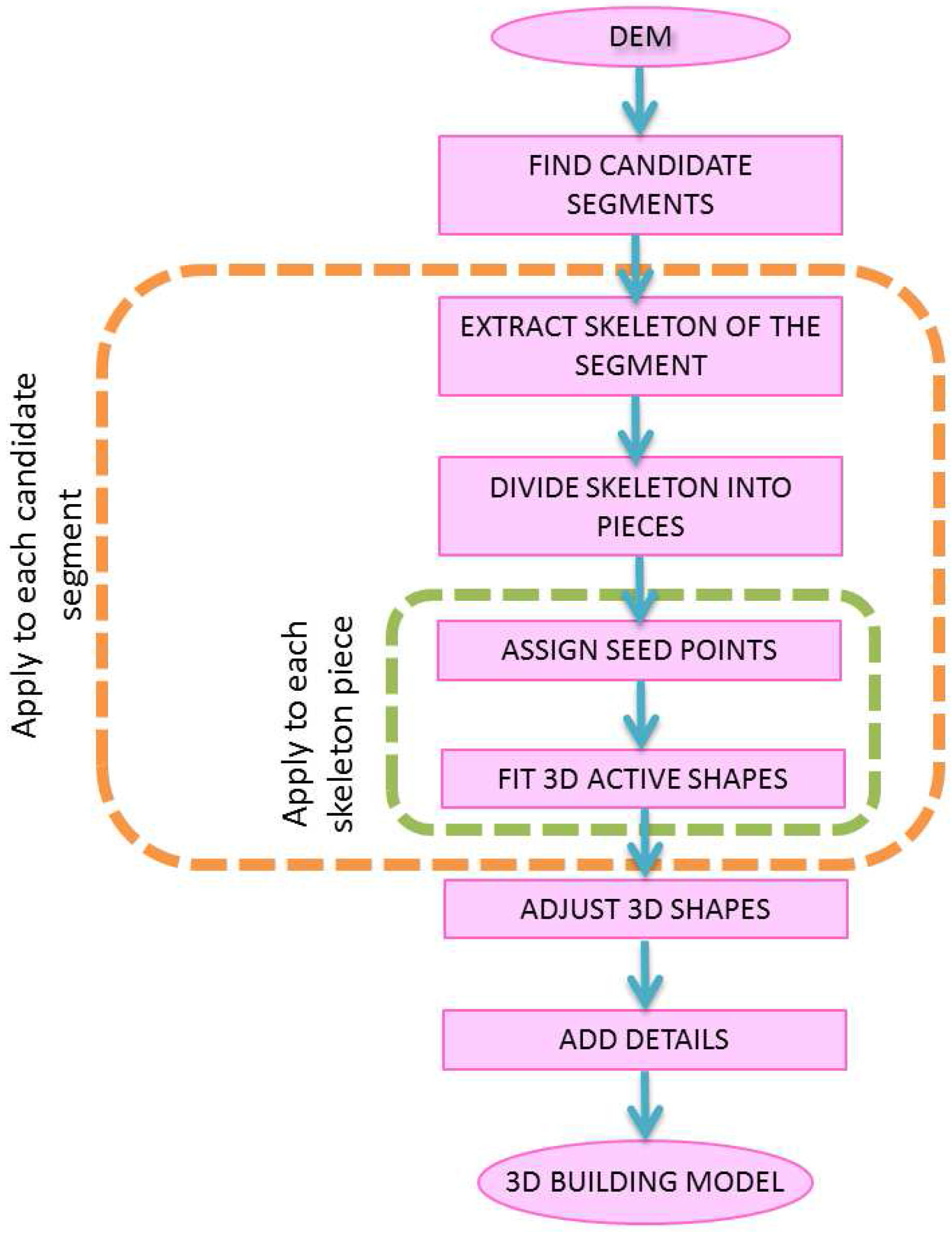
In Figure 1, we demonstrate the steps of the proposed algorithm in basic modules. The process starts by finding candidate segments. Next, we take each candidate segment and extract its skeleton. In order to simplify the 3D shape detection problem, especially for complex building segments, we divide the skeleton into pieces and process each skeleton piece separately. On each skeleton piece, we assign seed points. From each seed point, a 3D active shape start is initiated to grow and fit in the best possible position. After 3D active shape fitting is applied to all seed points in a building segment, the Adjust 3D Shapes module merges all 3D shapes, makes corrections when it is necessary and obtains a single 3D shape that corresponds to the 3D building reconstruction. Finally, in the Add Details module, it is possible to add details to the 3D model, such as facade texture or 3D rooftops, in order to increase the details of the building model and make it look more realistic. In the whole process, only in this module is human interaction necessary. In the following subsections, we explain each algorithm module in detail.
Figure 1.
Workflow of the 3D Building Model Generation Algorithm.
2.1. Extracting Approximate Building Footprint Segments
Before detecting the exact building footprint and modelling the 3D building structure, we start by finding segments which may corespond to a possible building footprint. If a normalized digital elevation model is available, objects which are higher than a constant value could be segmented by applying a simple height threshold, as a normalized digital elevation model contains the heights of the objects relative to the terrain elevation [23]. However, in most cases, only a DEM is available as input data and a normalize digital elevation model must be generated first which increases the computation load. Using simple thresholding on a DEM causes wrong segmentation results especially on hilly regions. Instead of calculating the normalized digital elevation model, in this study we choose to use local thresholding to the input DEM in order to detect the approximate location and footprint shapes of the buildings.
Figure 2.
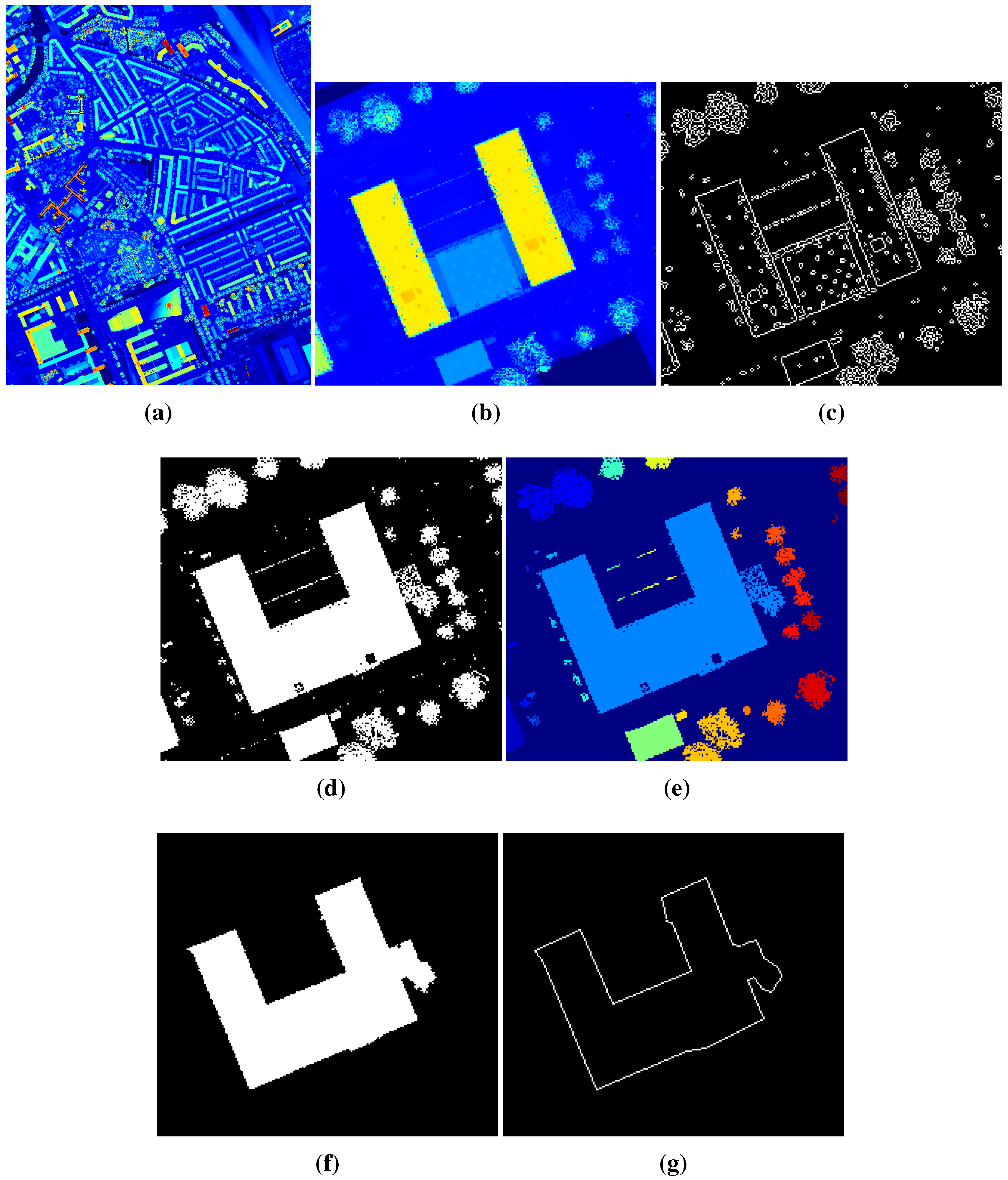
(a) Airborne laser scanning DEM of Delft city; (b) an example building to illustrate the steps of the proposed algorithm; (c) Canny edges of the DEM shown in (b); (d) local thresholding result for the DEM shown in (b); (e) connected components labeled with different colors for detected segments shown in (d); (f) the object of interest is chosen by removing the connected components that are smaller than a certain size threshold; (g) the result obtained by using a 2D active shape fitting approach presented in earlier work [13] (the neighboring tree is also detected as part of the building).
Figure 2.
(a) Airborne laser scanning DEM of Delft city; (b) an example building to illustrate the steps of the proposed algorithm; (c) Canny edges of the DEM shown in (b); (d) local thresholding result for the DEM shown in (b); (e) connected components labeled with different colors for detected segments shown in (d); (f) the object of interest is chosen by removing the connected components that are smaller than a certain size threshold; (g) the result obtained by using a 2D active shape fitting approach presented in earlier work [13] (the neighboring tree is also detected as part of the building).

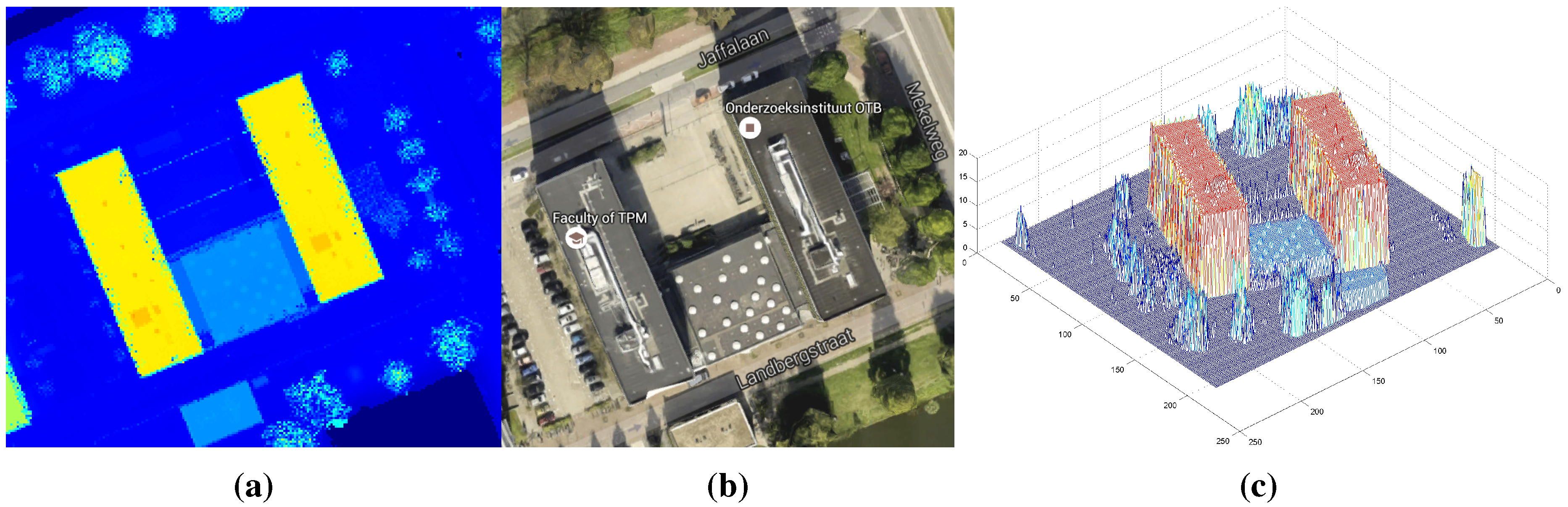
In Figure 2a, we show Airborne Laser Scanning (ALS) data sampling a part of Delft, The Netherlands. A DEM is generated by assigning the 3D laser measurement values to a gridded surface in order to generate an image file where the pixel brightness values correspond to the height value above sea level. Figure 3 shows a building selected from this area to illustrate the steps of the algorithm. Figure 3a,b shows the Google Street View and Google Earth images, respectively. Figure 3c shows the ALS data taken over this showcase building. In Figure 2b, a sub-part of the DEM () that is generated using ALS data is shown. In our application, we have used a -m grid size.
For local thresholding, a pixel size sliding window is used over the DEM, and a new threshold value is used for each window. This window size is chosen by considering approximate building sizes in the input DEMs. However, the thresholding result does not differ significantly with slight changes of window size or with slight changes of input image resolution. Therefore, it is possible to use the same window size for our input DEMs with different geometric resolutions.
After applying local thresholding to the example DEM, we obtain a binary result () where the pixels higher than the threshold value are labeled with a value of one. In Figure 2d, we show the local thresholding result () for the example DEM.
Segments are labelled using a connected component analysis [24], and small size components are eliminated, since they cannot represent buildings. Herein, we have selected the size threshold as 5000 pixels. However, the size threshold value must be selected considering the ground sampling resolution of the input DEM and minimum footprint sizes of the buildings in the study area. In Figure 2e,f, we present the result of the connected component analysis and size thresholding, respectively. As can be seen, small size segments corresponding to non-building objects are eliminated, and only building footprints are left. In this automatically-achieved result, the building footprints might have fluctuating borders depending on the quality of the input DEM. Besides, neighbouring trees might be detected as parts of the buildings, as it is also the case for our example building footprint in Figure 2g, which shows the building footprint detection result obtained by the previous active shape approach [13].
Figure 3.
(a) A Google Street View of the showcase building; (b) a Google Earth view of the show case building; (c) the original ALS DEM.
Figure 3.
(a) A Google Street View of the showcase building; (b) a Google Earth view of the show case building; (c) the original ALS DEM.

2.2. Assigning Seed Points
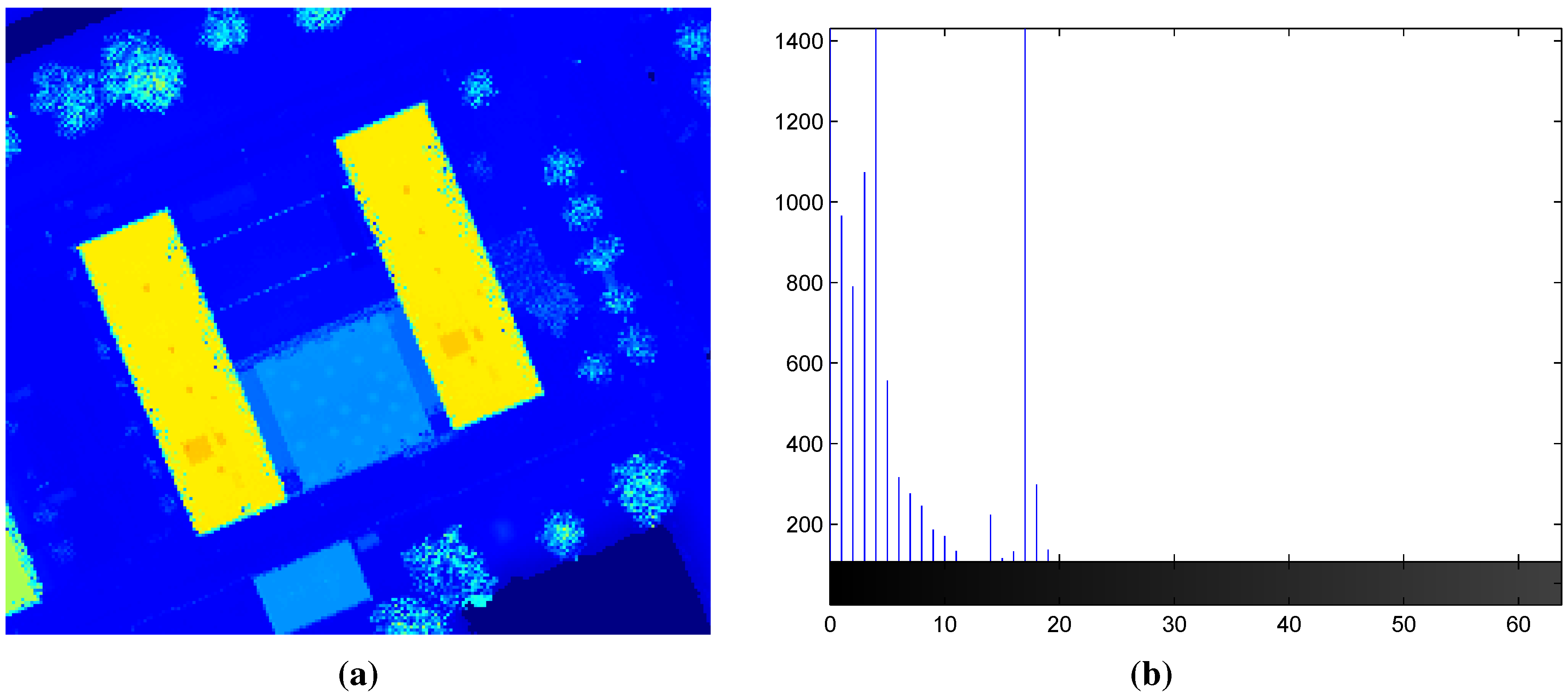
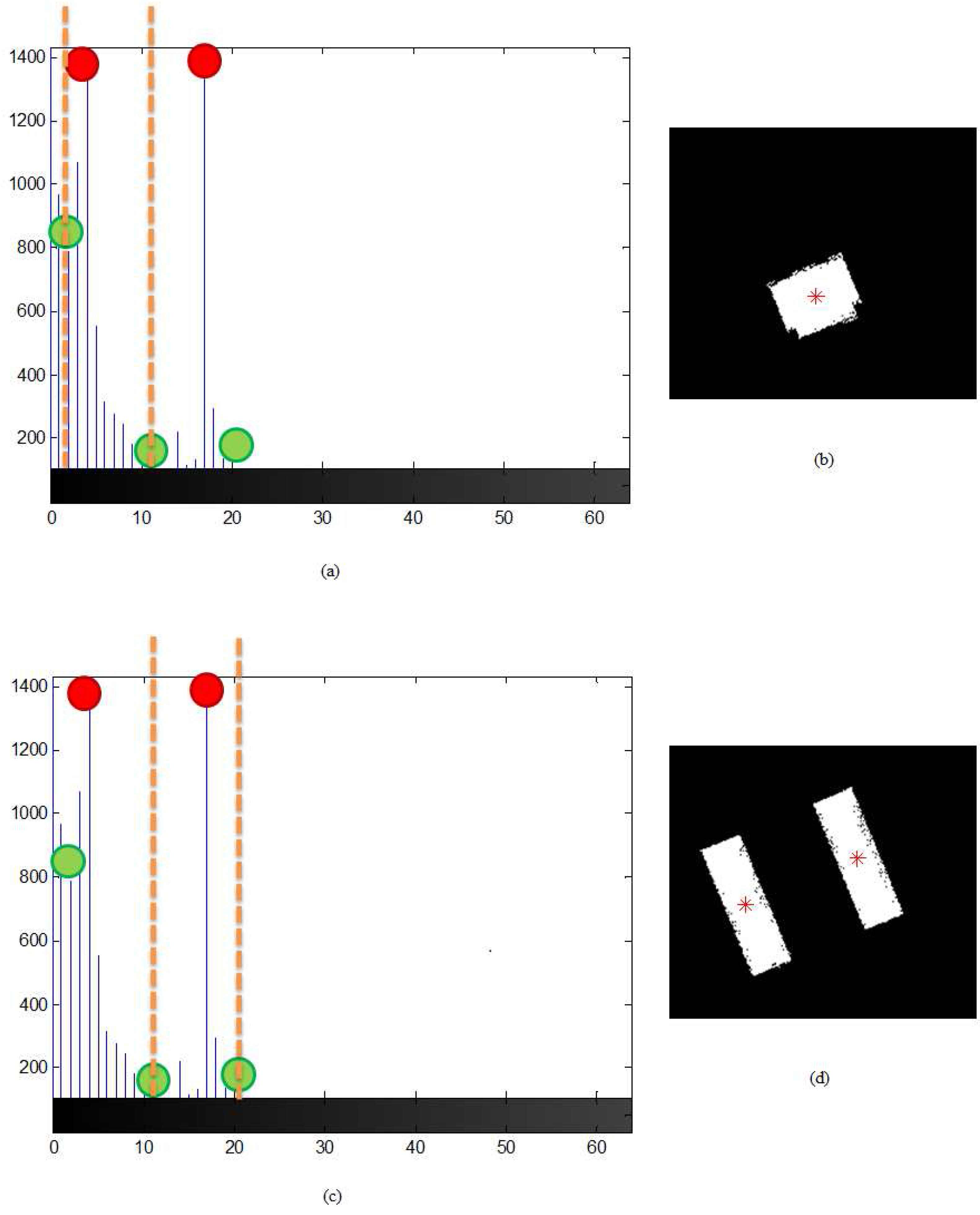
For each approximate building footprint segment, as obtained by the previous step, a height histogram is generated as the example one in Figure 4a. The horizontal axis of the histogram shows the elevation of the pixels in the DEM in meters. We have chosen 1-m bins for this representation. The vertical axis of the histogram shows how many times a height value appears in the DEM.
We use the local maxima of the histogram to distinguish building parts with a uniform height. To do so, each sequential local minimum pair is used for thresholding. In this way, building segments with different height values are distinguished. After this segmentation, for each segment, it is evaluated whether it is a simple shape. A method for testing the building footprint shape complexity is proposed in Sirmacek et al. [14]. In their approach, a shape is considered complex if it contains inner yards (holes). They make this decision by computing the Euler number of the binary building segment. The Euler number of a binary object is defined as the total number of objects (equal to one when only one building segment is taken) minus the total number of holes in those objects. If the Euler number is zero or below, the building segment is considered complex.
Figure 4.
(a) Airborne laser scanning based generated DEM data of the showcase building, (b) Height histogram for the given DEM. (The horizontal axis shows the elevation of the pixels in the DEM in . The vertical axis shows how many times a height value appears in the DEM.)
Figure 4.
(a) Airborne laser scanning based generated DEM data of the showcase building, (b) Height histogram for the given DEM. (The horizontal axis shows the elevation of the pixels in the DEM in . The vertical axis shows how many times a height value appears in the DEM.)

The following steps are used to estimate the model. The building segment is divided into elongated pieces using its skeleton, as described in [15,25]. To do so, junctions and endpoints of the building segment skeleton are extracted using basic morphological binary image processing approaches as they are introduced by Yung and Rosenfeld [26]. A junction is defined as a skeleton pixel that has more than two incident pixels. An endpoint is defined as a skeleton pixel that has only one incident pixel. The skeleton is divided into pieces by removing these junction pixels from the skeleton. Furthermore, each obtained skeleton piece is divided into pieces of l pixels in length maximally. Center pixels of the obtained skeleton pieces are chosen as seed-point locations to run the active shape growing algorithm. If the building segment is simple, a seed point is put at the center of mass of the shape. In [25], the segmentation, skeleton and seed point extraction steps are demonstrated on a complex building structure.
For our showcase building, the automatically-extracted initial seed points are shown in Figure 5b,d. After initial seed point selection, in the next step, we use each seed point location for growing a virtual 3D active shape model.
Figure 5.
(a) Thresholding cut-offs for the first and the second local minima of the height histogram, (b) the seed point location found by using the cut-offs given in (a), (c) thresholding cut-offs for the second and the third local minimums of the histogram, (d) the seed point locations found by using the cut-offs given in (c).

2.3. Fitting 3D Active Shape Models
3D active shape models are fit on the input DEM, by growing them starting from the detected initial seed point locations. Active shape model fitting is done by growing a virtual cube shape starting from a seed point, until the 3D shape model finds the best orientation and size which is evaluated in terms of reaching to the maximum value using a suitable energy function.
Sirmacek and Unsalan [13] proposed an automatic 2D rectangular shape approximation approach using previously-extracted Canny edges [27]. To fit rectangular active shapes to buildings, they start to grow the active rectangular shape on each seed point location . When the active rectangular shape grows in the θ direction and hits a Canny edge, the growing process is stopped, and an energy value is calculated. This process is repeated for the same seed point for different θ directions and each time the energy value is computed.
Here, we propose to improve this approach by modifying the previously-proposed energy equation in order to incorporate height information, as well. By considering the height information in the active shape growing process, the new energy formula becomes as follows:
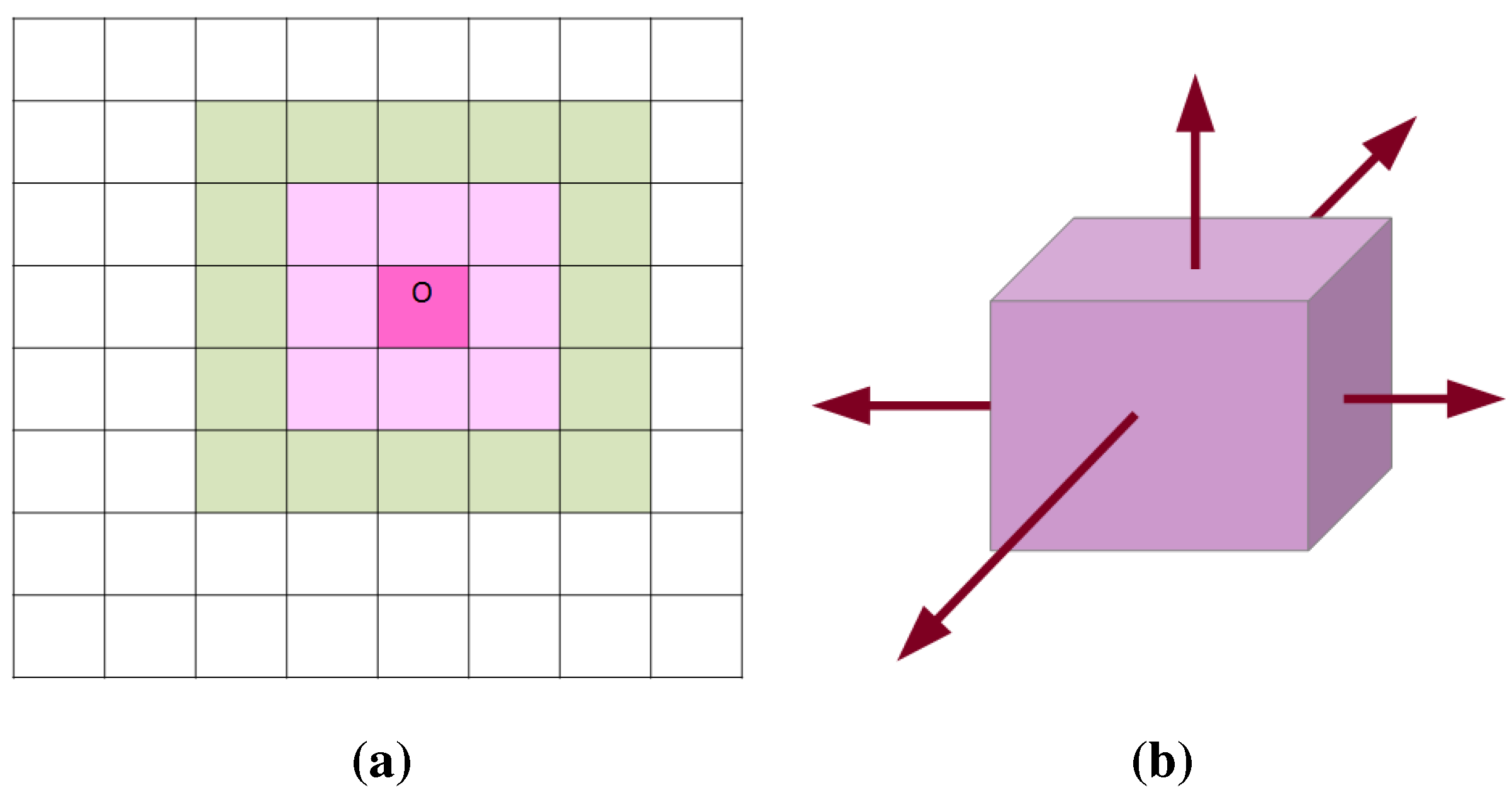
Here is the new energy value, which is computed at each growing iteration for four () vertical edges of the virtual box. In the formula, corresponds to the pixels that are inside the virtual box (the initial position of the virtual box, is indicated by the pink pixels in Figure 6a). Therefore, shows the mean of the height value inside the virtual box. denote the neighbour pixels of the l-th vertical box edge that are outside the virtual box (the initial position of the virtual box, is indicated by the green pixels in Figure 6a). Therefore, the value suddenly becomes very large when the l-th vertical box edge becomes very close to a building edge (because of the height difference between the rooftop and the terrain). In order to stop the growing of an edge at the right moment, we set a threshold value which is equal to 3 m in our application. So if the mean height of the inner pixels and the mean height of the outer pixels in the growing direction differ more than 3 m, we stop growing the virtual box in that direction. At each growing iteration, after four vertical edges are checked with respect to the energy test given in Equation (1), we assign the final value as the height of the virtual box. Therefore, the virtual box has actually five growing directions as illustrated in Figure 6b.
Figure 6.
(a) Illustration of a 3 × 3 pixel virtual box footprint at the initial position (magenta color center pixel represents the seed point at , pink pixels represent the pixels inside the virtual box borders, green pixels represent the pixels which are the outside neighbours of the virtual box borders), (b) Illustration of a 3D virtual box with 5 growing directions are indicated by arrows.

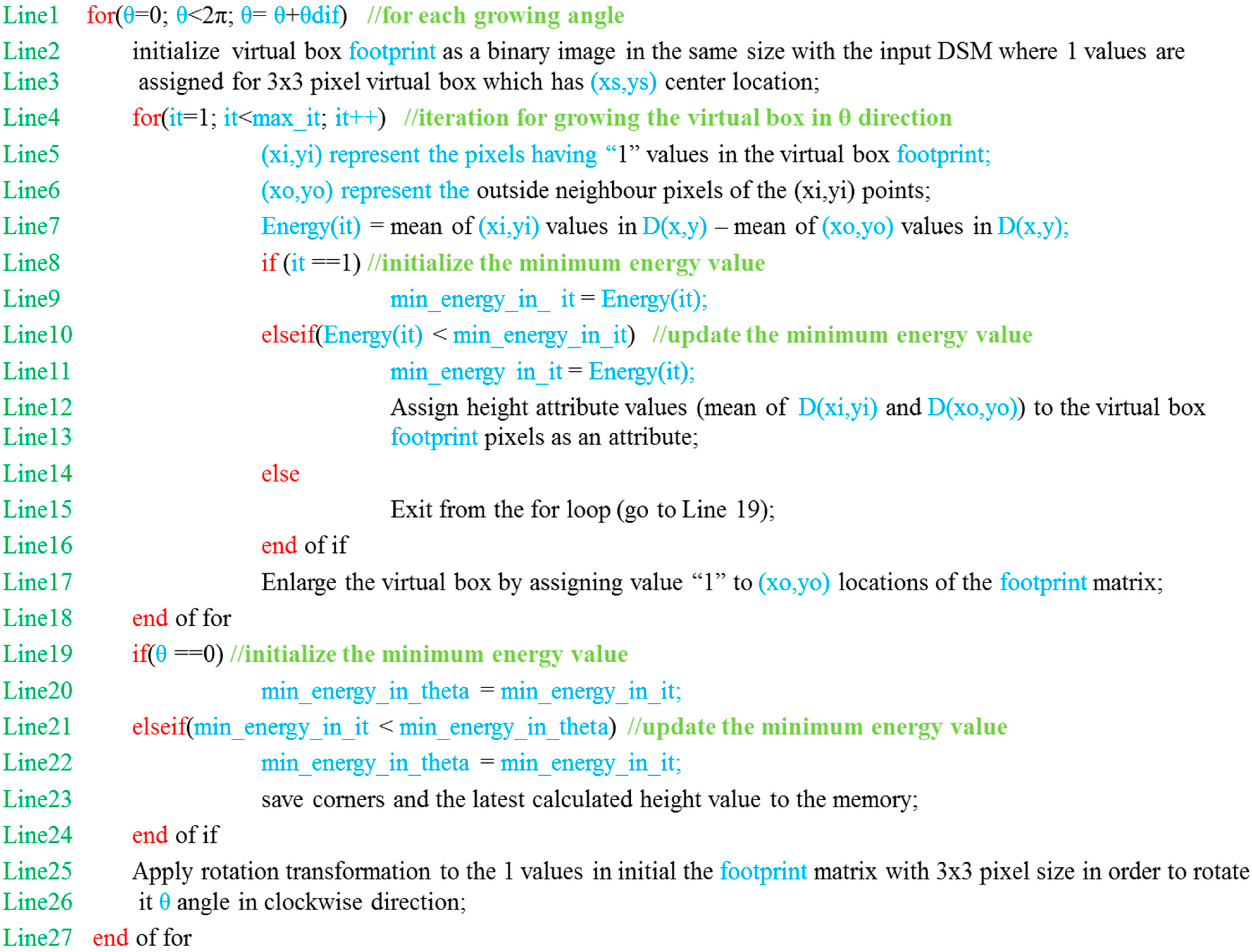
In Figure 7, we provide pseudocode for the 3D virtual box fitting algorithm. The algorithm includes two main loops; one for iteratively pushing the borders of the virtual box in the outward direction (the “for” loop at Line 4) and one for changing the angle to the next growing orientation after reaching the minimum energy value in the current growing orientation (the “for” loop at Line 1).
Figure 7.
Pseudocode of the 3D Virtual box growing function.
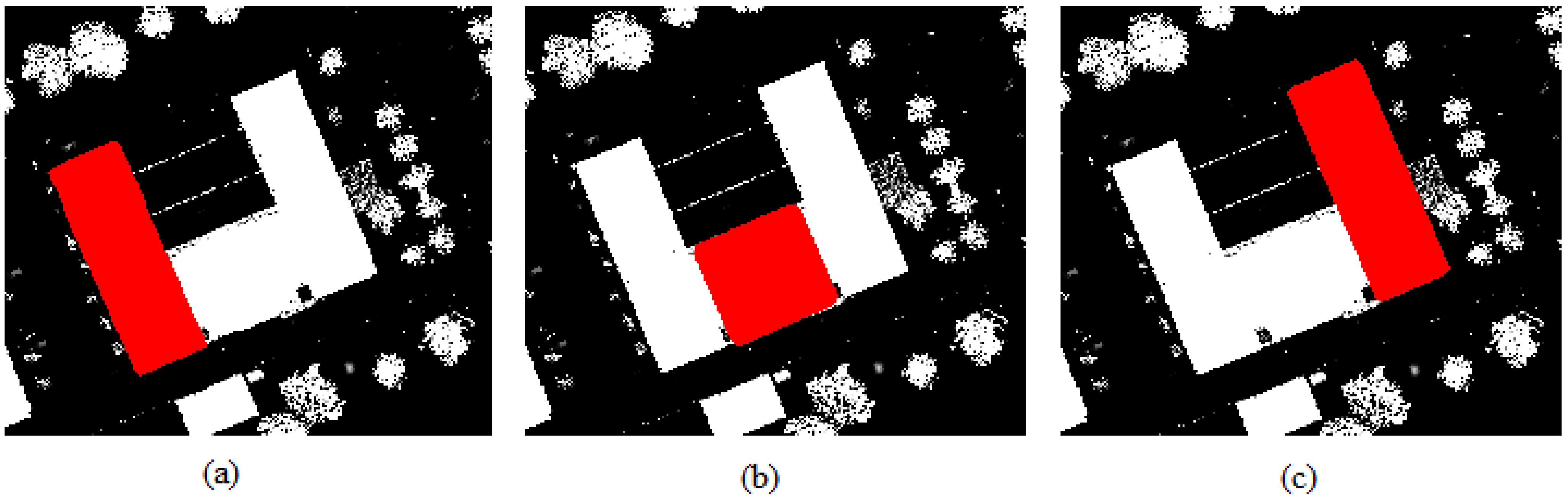
In Figure 8, we show the footprints of the 3D active shape fitting results of the virtual shapes that have started growing on the initial seed points.
Figure 8.
The sub-figures (a–c) show the footprints of 3D active shape fitting results of the virtual shapes which have started growing on the initial seed points.
Figure 8.
The sub-figures (a–c) show the footprints of 3D active shape fitting results of the virtual shapes which have started growing on the initial seed points.

2.4. Completing the 3D Model
After obtaining the 3D models that fit into the building positions starting from the initial seed point locations, the building footprint might still have some areas that have not been considered in the model. Therefore, the Adjust 3D Shapes module (as shown in Figure 1) determines new seed points and calls the 3D active shape method for the new seed points in order to complete the building model.
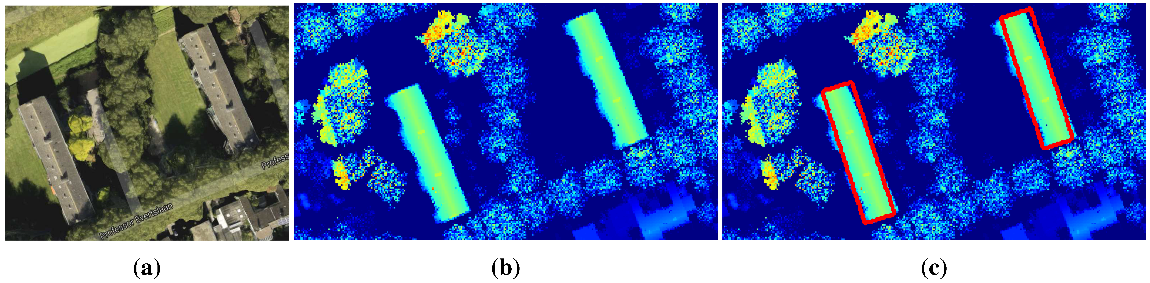
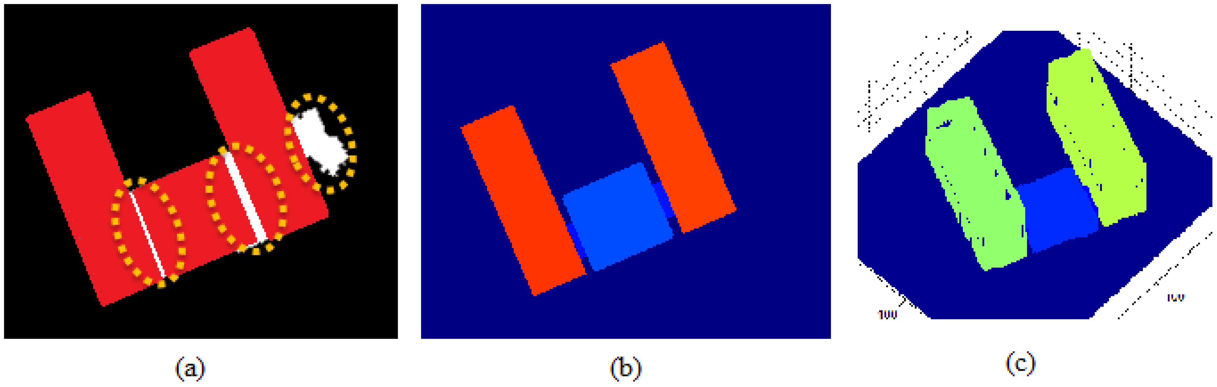
In Figure 9a, the red pixels show the building footprint that is automatically detected using the 3D active shape growing approach starting from the initial seed points. As indicated by the dashed circles, there are still some regions in the building segment that are not taken into account for active shape growing. In order to complete our 3D model, in this step, we consider the parts of the building segment that are not labeled by the building footprint in the previous step. To do so, we take each unlabeled segment as indicated in Figure 9a by the dashed yellow circles. For each segment, again, the previous analysis is applied. That means that, for each segment, first the shape complexity is tested. If the building segment is considered complex, then it is divided into elongated pieces, and new seed points are inserted into the center of mass of each piece. If the segment is not complex, then simply one new seed point is inserted in its center of mass. After applying this analysis on each segment indicated by the yellow circles, we run the 3D active shape growing approach on these new seed points as a second run in our 3D modeling application. The obtained building footprint and the 3D model are represented in Figure 9b,c, respectively. In this example, an important strength of the new active shape growing approach is demonstrated. In Figure 9a, the segment at the right-most side actually comes from a tree that is very close to the building. As can be seen in the example given in Figure 2f,g, this tree cannot be separated from the building footprint with the 2D active shape growing approach. However, the new 3D active shape growing approach can eliminate this tree segment, since the varying height of the segment does not allow the virtual 3D box shape to fit to the segment.
Figure 9.
(a) Approximate building footprint segment regions indicated by yellow dots are not covered by the active shape growing results on the initial seed points; (b) the final 3D model after growing active shapes also starting from the second seed point selection process results (top view); (c) the final 3D model (3D view).

Since modern buildings are frequently built using different geometries (instead of just simple rectangular shapes), there might be other challenges depending on the scene. For example, it might be possible to have buildings that have X-shaped footprints or segments at different angles. In such a case, the intersection points of the elongated segments will generate junctions in the skeleton, which will help to divide the skeleton into elongated pieces. Afterwards, the seed points will be assigned to the elongated segments, and each segment will have a 3D active shape model fitting result. When the building segments have different angles, the most important issue will be choosing the steps between different θ growing directions. It would be possible to obtain more accurate 3D fits when the is smaller; however, that would require more computation time, as well. The link between the 3D modeling accuracy and the is discussed in the Experiments Section in more detail.
2.5. Other Possible Improvements
Having obtained the 3D building models, it is possible to increase the details and reality of the models by adding a rooftop model and texturing the building facade with Streetview pictures. Here, we present an example.
2.5.1. Adding Coarse Building Rooftops to the 3D Model
In this study, we do not specifically focus on the details of rooftop construction; however, after detecting building models, it is possible to add coarse rooftop models on the building models. As presented in an existing study [15], as a first step, the building rooftops are classified simply as flat or gable. The obtained information is useful to insert 3D roof models. This classification is done by checking the ridge-line information. The ridge-lines are detected using a derivative filter [15]. If there is not enough ridge-line information detected then the rooftop is classified as “flat roof”, it is classified as “gable roof”. Ridge-line extraction and rooftop classification methods are discussed in Sirmacek et al. [15] in detail. Adding rooftop models is also applied in a similar way by Xiong et al. [28]. Zang et al. [29] used satellite images to train an image classifier in order to understand the rooftop type and model 3D roofs, which can add a more realistic look to the 3D urban models. Those rooftop reconstruction methods are useful to obtain models easily when the rooftop structure is not very complex, that is composed of simple planes. However, more complicated rooftops, which include towers and different geometrical primitives, cannot be reconstructed with these approaches.
2.5.2. Adding Facade Texture on 3D Model
For realistic 3D rendering, adding facade texture is crucial. Adding facade texture can cause a magical effect on the human visual system. Covering the simple 3D building model with a realistic facade image gives the impression that many tiny details are added to the model, although we do not add any structural features. Herein, we propose a very simple building facade texturing method in order to make the 3D models look more realistic while they can still be easily rendered. To do so, we use an approach similar to the semi-automatic method proposed by Lee et al. [30]. In our study, we used Google Street View images as ground images, which enables the user to texture the models even without needing to go to the study area to acquire pictures. Instead of extracting the lines and the vanishing points, herein, we ask the user to select a polygon area in the Google Street View image and to select the building facade in the 3D model that is going to be textured. Then, the selected polygon is automatically stretched and used for texturing the facade. This is done by calculating the transformation function using the corner points of the polygon on the 2D Google Street View image and the corresponding corner points of the polygon on the 3D surface to be textured. The transformation function applies 3D translation, rotation and scaling. Transformation function extraction is done as presented by Hesch and Roumeliotis [31]. After calculating the transformation function using the tie points (the polygon corners), the same function is used to register all 2D image points on the 3D surface. The linear interpolation function of MATLAB software is used for texturing the waterproof 3D surface.
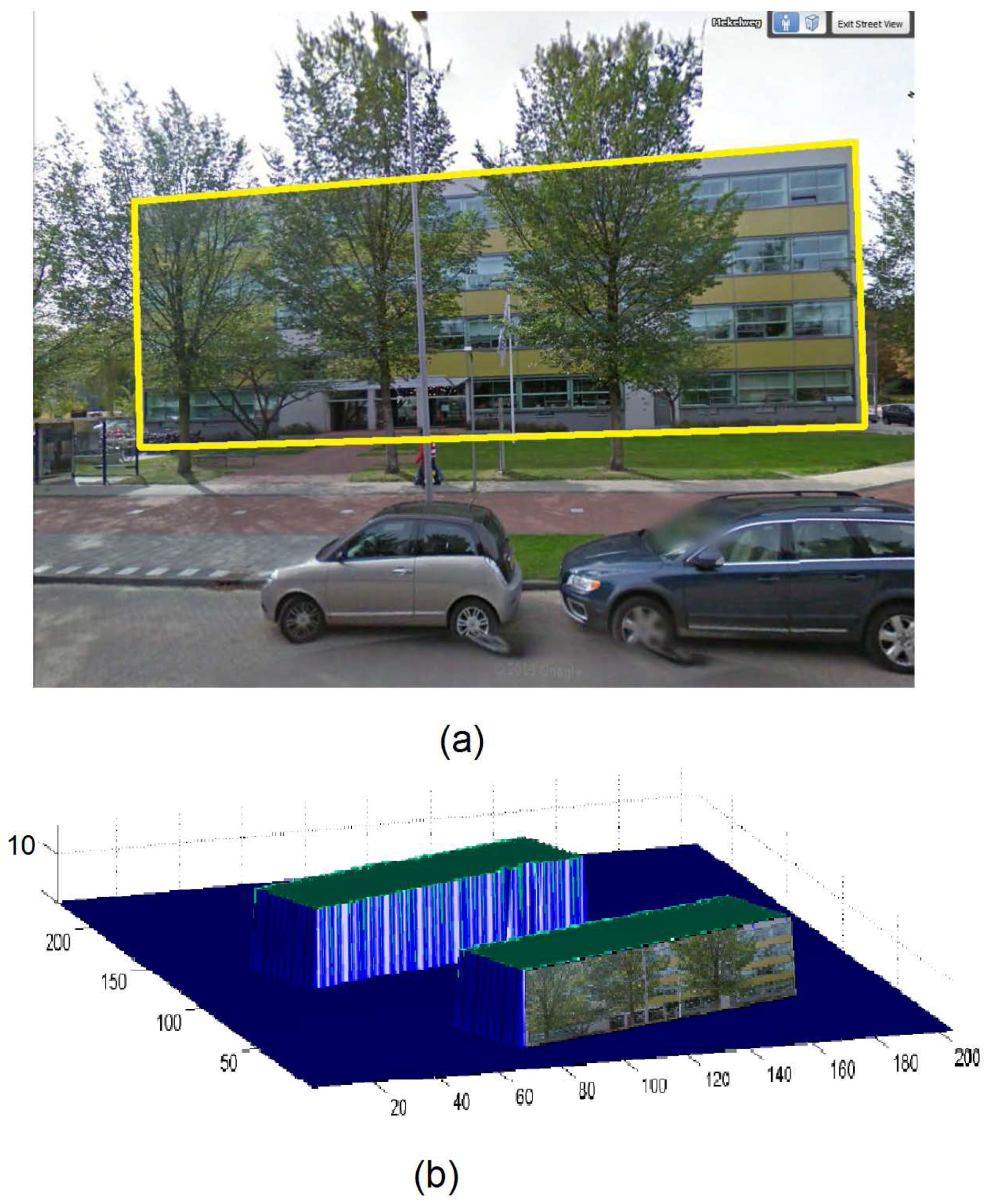
A Google Street View image and the selected polygon are shown in Figure 10a. In Figure 10, we see the 3D model after the polygon is stretched and used for texturing the selected facade. Unfortunately, using this approach, we cannot prevent the registration of trees, cars or other occluding objects on the 3D building model. One idea might to use multiple Google Street View images and to try to obtain the facade texture by eliminating the occluding objects. We plan to focus on this problem in our future studies.
Figure 10.
(a) The facade polygon area is selected by the user on the Google Street View image; (b) 3D model of the showcase building from Delft University of Technology. The building facade of the model is textured using the selected polygon area in the Google Street View image.
Figure 10.
(a) The facade polygon area is selected by the user on the Google Street View image; (b) 3D model of the showcase building from Delft University of Technology. The building facade of the model is textured using the selected polygon area in the Google Street View image.

3. Experiments
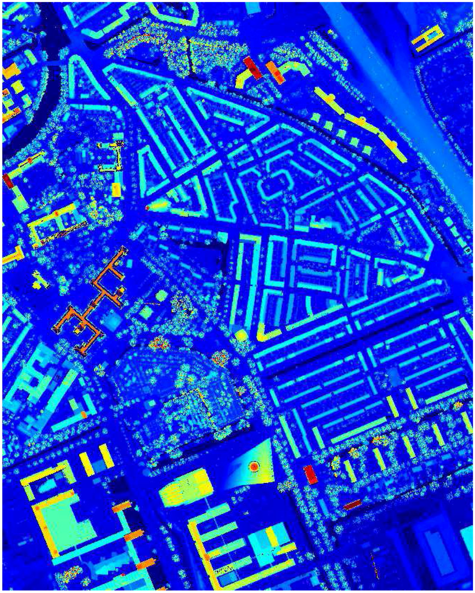
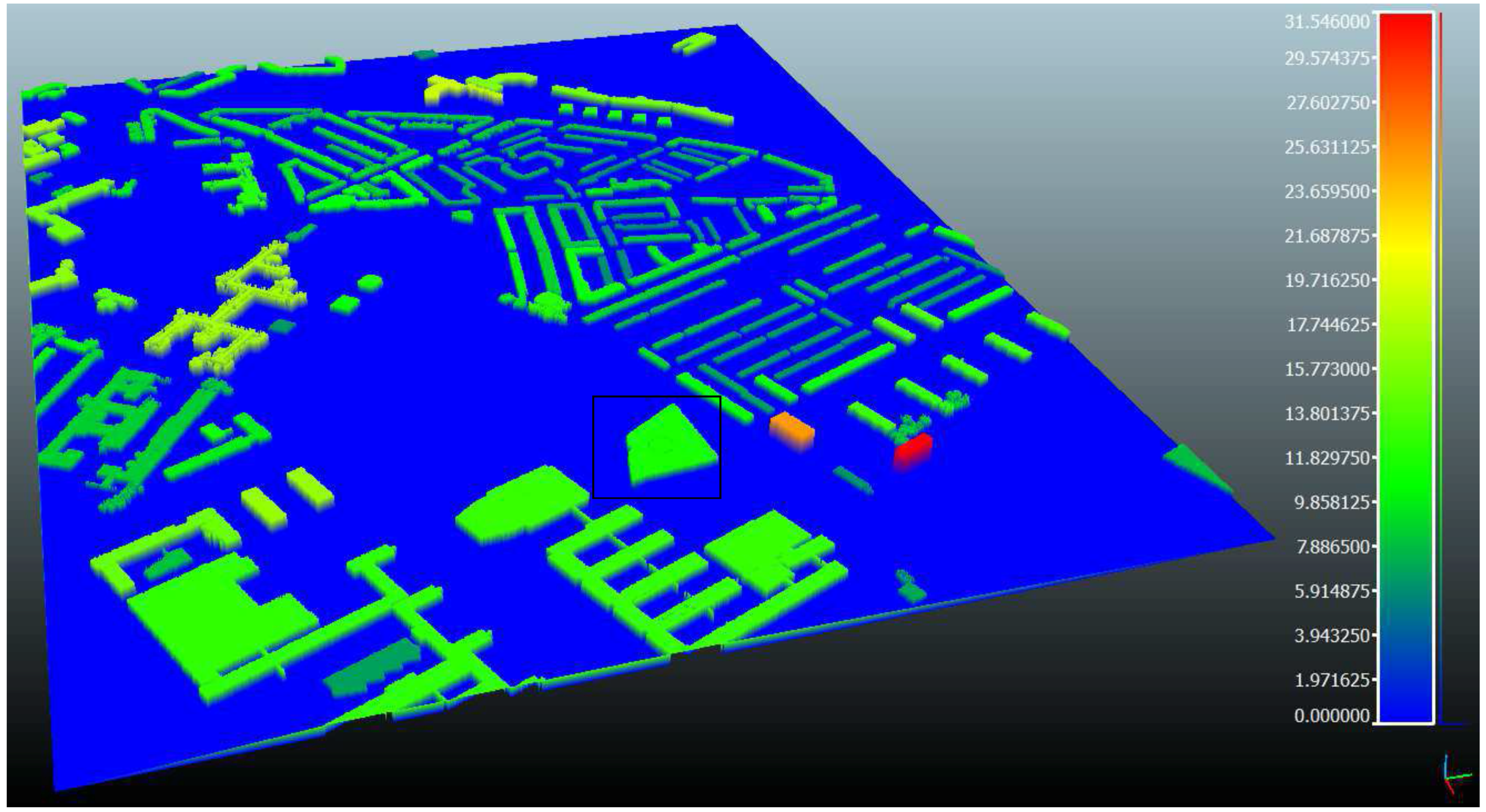
As input, we have used the Actual Height model of the Netherlands (AHN2) data from the Dutch airborne laser altimetry archive. These data were acquired between 2007 and 2008 [32,33,34]. They have a point density of 10 points per square meter . A top view of the input data is shown in Figure 11.
Figure 11.
Top view of the ALS data acquired over a part of Delft, The Netherlands. The points are false colored to show height differences. Here dark blue corresponds to the lowest and red corresponds to the highest values in z-dimension.
Figure 11.
Top view of the ALS data acquired over a part of Delft, The Netherlands. The points are false colored to show height differences. Here dark blue corresponds to the lowest and red corresponds to the highest values in z-dimension.

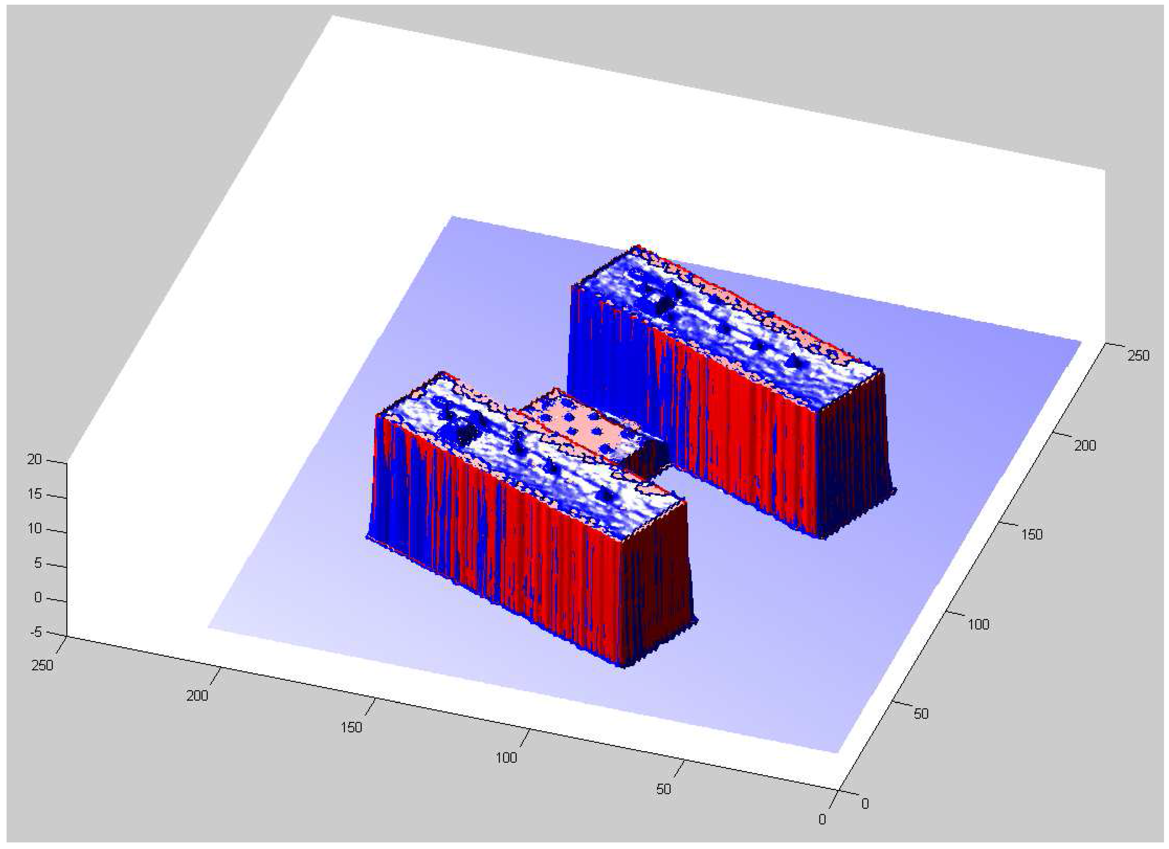
In the previous sections, we have introduced the algorithm steps on the showcase building (). In order to give an idea about the difference of the 3D model and the original input data, in Figure 12, we show them together. In this image, the red surface corresponds to the height values of the automatically-generated 3D model, and the blue surface corresponds to the height values of the raw input data. As can be seen in this figure, the original input data include many objects on the building rooftop, which increases the difficulties for quick rendering and data storage.
Figure 12.
Red surface; height values of the automatically generated 3D model. Blue surface; height values of the raw input data.
Figure 12.
Red surface; height values of the automatically generated 3D model. Blue surface; height values of the raw input data.

In this section, we also present more results of the proposed 3D reconstruction method. In Figure 13a, we show , and in Figure 14a, we show . In Figure 13b and Figure 14b, we show the Canny edges detected from the input DEMs. These results show us the great difficulty in detecting building footprint edges with well-known image processing algorithms. However, the building footprints are clearly detected by the 3D active shape growing approach, as can be seen in Figure 13c and Figure 14d. A zoom into the virtual box footprint in Figure 14c shows us that the very high spatial sampling of the input data even represents very small details of the structure, like balconies. Figure 15 shows the result footprints when the algorithm is applied on the full input DEM (instead of testing it only on the segment). The resulting footprint does not include balconies and neighboring trees. The detection of tree clusters as a building is also prevented by the 3D active shape growing approach.
Figure 13.
(a) DEM of the region which includes , (b) Edges detected from DEM by applying Canny edge detection method, (c) The building footprint which is detected by the 3D active shape growing approach.
Figure 13.
(a) DEM of the region which includes , (b) Edges detected from DEM by applying Canny edge detection method, (c) The building footprint which is detected by the 3D active shape growing approach.
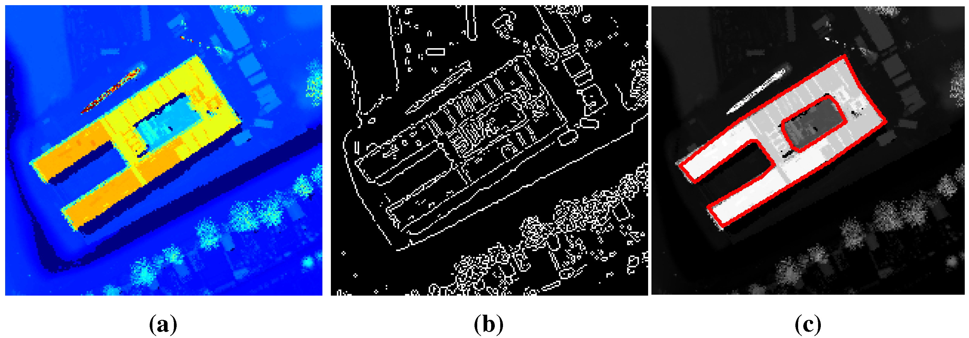
Figure 14.
(a)DEM of the region which includes , (b) Edges detected from DEM by applying Canny edge detection method, (c) A zoom into the final footprint of the virtual box, (d) The building footprint which is detected by the 3D active shape growing approach.
Figure 14.
(a)DEM of the region which includes , (b) Edges detected from DEM by applying Canny edge detection method, (c) A zoom into the final footprint of the virtual box, (d) The building footprint which is detected by the 3D active shape growing approach.
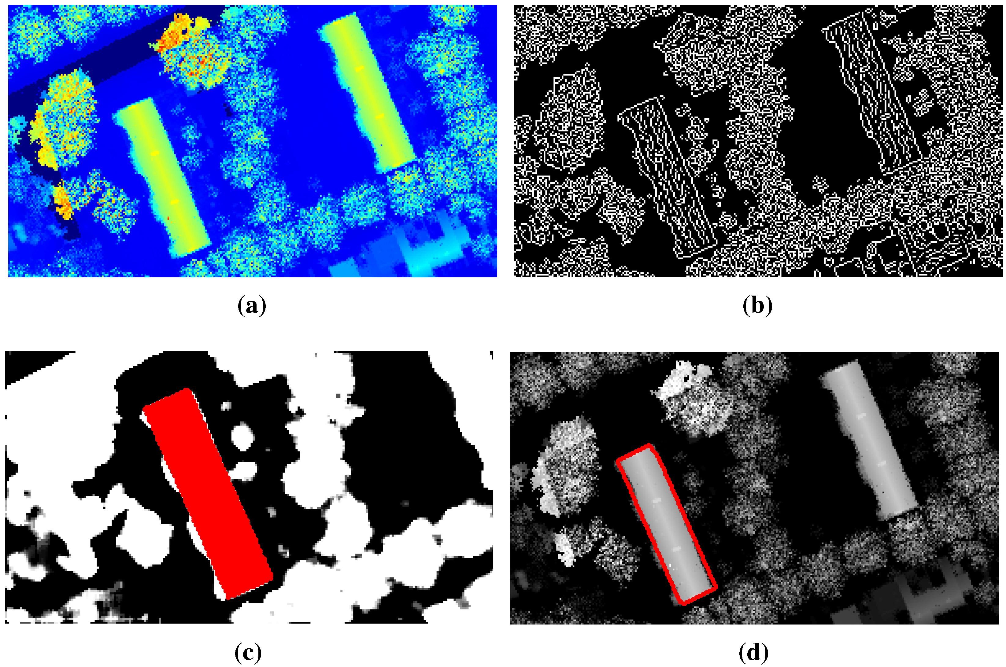
Figure 15.
(a) Google earth view of an example study region, (b) DEM of the same region obtained by ALS sensor data, (c) Automatically detected 3D model footprints.
Figure 15.
(a) Google earth view of an example study region, (b) DEM of the same region obtained by ALS sensor data, (c) Automatically detected 3D model footprints.
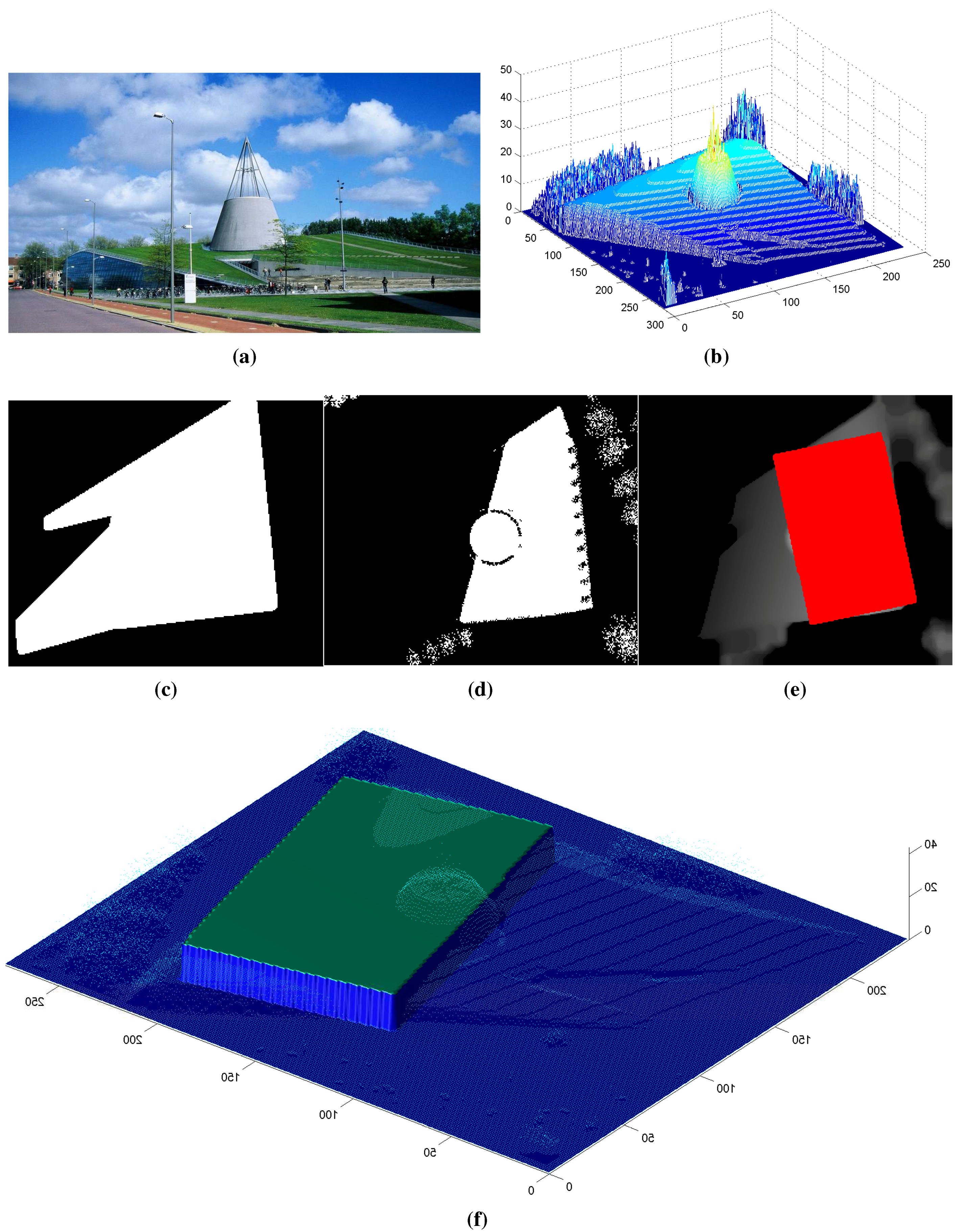
In order to represent an example of challenging reconstruction situations, we have applied the algorithm on a complex building with an irregular rooftop. The chosen building (TU Delft library building), which we label as , is represented in Figure 16. Here, Figure 16a shows the street view and Figure 16b shows the DEM of the building, which is acquired from ALS. As can be seen in these pictures, the building has a slope-like rooftop, which reaches the ground at one side of the building. Besides, there is a cone shape structure in the middle of the building. In Figure 16c, we show the actual building footprint, which is prepared manually by an expert. In Figure 16d, we show the automatically-extracted approximate building segment. A seed point is located in this segment. The resulting footprint and an oblique 3D view of this initial virtual box fitting result can be seen in Figure 16e,f, respectively. Since the result does not cover the complete footprint segment, new seed points are assigned to the footprint parts, which are not covered by the initial virtual box fitting result. The final reconstruction result of this complex building is labeled by a square in Figure 17.
In Table 1, we tabulate quantitative results from the experiments on three different building structures. In this table, Columns 2 and 3 show the building footprint complexity and the rooftop type. Column 4 shows the number of building footprint data in the reference footprints that were generated by us manually. In Columns 5 and 6, we show the true footprint detection results of the 3D active shape growing algorithm as the number of pixels and as a percentage. Column 7 shows the percentage of false alarms that are coming from pixels that are detected by the 3D active shape growing algorithm, but that do not appear in the reference footprint. Finally, in the last column, we represent the height estimation error in meters. This is calculated by checking the mean of the height differences between the original input and the reconstruction result in the intersecting footprint. The table shows the robustness of the method on the first three of the complex building structures. The low height error for the gable rooftop building example shows that the height error can be ignored when very high precision in reconstruction is not necessary. represents an irregular building structure example, which has neither a flat nor a gable-shaped rooftop, but curved instead. Since one half of the building is very close to the Earth’s surface, the building model fits only the higher part. Therefore, as is seen in detected pixels column of Table 1, almost half of the building footprint pixels are detected by the automatic modeling approach. On the other hand, there is a very small number of false alarm pixels, which can be ignored. For , the height error is quite high compared to the error of the other three models. One of the reasons is that it is not possible to fit a flat rooftop on this building with a curved rooftop. Another reason is that the cone-shaped high structure in the middle of the building cannot be reconstructed; however, it increases the error of the difference when the original DEM measurements are compared to the automatically-reconstructed models.

| - | Shape | Roof | Pixels | Detected | TD (%) | FA (%) | |
|---|---|---|---|---|---|---|---|
| Simple | Flat | 9279 | 8856 | 95.44 | 3.19 | 0.13 | |
| Complex | Flat | 5034 | 4363 | 86.67 | 0.77 | 0.04 | |
| Simple | Gable | 1980 | 1889 | 95.40 | 3.53 | 0.02 | |
| Complex | Irregular | 30694 | 14329 | 46.68 | 1.01 | 2.60 |
Figure 16.
(a) Street view of TUDelft Library (), (b) DEM of the same building obtained by ALS sensor data, (c) Manually labelled building footprint, (d) The initial virtual box fitting result, (e) automatically detected 3D building model footprint, (f) 3D oblique view of the automatically reconstructed model.

Figure 17.
The automatically obtained 3D model as a result of the proposed approach. (The final reconstruction result of the library building in Figure 16 is indicated by a square label.
Figure 17.
The automatically obtained 3D model as a result of the proposed approach. (The final reconstruction result of the library building in Figure 16 is indicated by a square label.

Since decreasing the value (increasing the number of different tested angles) might help with increasing the footprint detection precision, we apply a test on the simple building shape () by changing the value for 3D active shape growing. In Table 2, we tabulate the footprint detection performances by listing the True Detected pixels (TD) and False Alarms (FA). Besides, in column , we show the computation time (in seconds), which is needed to compute the final footprint. The computation times increases linearly with the increase of the growing directions. However, looking at the footprint detection performances, it is possible to say that the usage of very small angle differences is not necessary, since using very small incremental steps does not result in significantly better performance, although it requires more computation time.
| TD (%) | FA (%) | ||
|---|---|---|---|
| 94.89 | 0.02 | 15.19 | |
| 95.68 | 1.46 | 9.62 | |
| 95.40 | 3.53 | 4.96 | |
| 92.02 | 9.24 | 3.51 | |
| 87.12 | 3.68 | 2.02 |
Finally, in Figure 17, we provide the automatic 3D modeling result for the test data. As can be seen, some of the buildings are missing, since there are no seed points assigned to them at the approximate footprint extraction step. This is mainly because of the size and height threshold that we have set for detecting the approximate building segment areas. If the buildings are not high and large enough to be detected at the initial seed point assignment step, they cannot be detected. It is possible to lower the size and height thresholds of the algorithm, in order to detect most of the missing buildings; however, this change would cause false detection of tree clusters as buildings, as well. When a vegetation index is not available to distinguish tree clusters from small-sized buildings, the algorithm cannot accurately find and reconstruct those buildings. In the future, we will focus on developing algorithms for quick segmentation of trees and tree clusters from laser scanning data, in order to eliminate the possible errors coming from their appearance and to be able to detect small buildings accurately, as well.
In order to be able to talk about the performance of the results, we have generated a binary mask by labeling the buildings manually. In Table 3, in the first column, we give the total number of buildings that are present in our mask. True Detection (TD) and False Detection (FD) numbers are calculated by comparing the automatic detection results with the mask. The table shows the results for the object-based comparison. Considering the building shape and size variety in the large test area, the evaluation results indicate possible usage of the proposed approach to generate 3D models of cities when simplistic representation of the buildings is necessary.
Table 3.
Performance tests for the automatic 3D modeling result given in Figure 17. TD, True Detection; FD, False Detection.
| # of Buildings | TD | TD (%) | FD | FD (%) |
|---|---|---|---|---|
| 224 | 175 | 78.12 | 16 | 7.14 |
We have also used the previous (2D active shape growing based) approach on the input data of . We have extracted quantitative measurements on the building footprint detection accuracy by comparing the result to the ground truth data. The accuracy measurements (TD) and (FP) are calculated as and , respectively. For the example building, higher accuracy with the 2D active shape growing-based approach is obtained because of the low building sections and connections, which are ignored by the 3D active shape growing-based approach, since they did not have sufficient height to be detected as a building part. On the other hand, the previous approach caused having a larger amount of false detections, since the neighboring trees are detected as a part of the building. These quantitative results of the building footprint detection accuracy can be compared to the results of the new algorithm, which is provided in Table 1.
4. Conclusions
Automatic modeling of 3D building models is very important for disaster management, simulation, observation and planning applications. 3D modeling with CAD tools is time consuming, especially when large cities with many buildings are modeled. Therefore, automatic algorithms are required. Herein, we introduced a method for automatic 3D building modeling based on a 3D active shape fitting algorithm.
The main novelties and contributions are summarized as follows:
1. Using the new 3D active shape growing approach, building shape detection robustness is improved. Test results showed that the proposed approach’s performance was superior compared to a previous shape detection method, especially when there are objects around the building that are adjacent to the building facade.
2. Very complex building models are constructed as a group of 3D box primitives. Being able to construct structures from primitives gives the opportunity to make a primitive model library, including different 3D shapes (such as cones, cylinders, etc.), and increases the desired details in 3D models in the future.
3. Instead of rendering very dense full point clouds, it is possible to use reconstructed 3D models that have a relatively small number of points and that still represent a realistic scene. This capability gives the possibility for easy rendering of a 3D model of a large area.
For testing the proposed approach, we used Airborne Laser Scanning (ALS) data sampling buildings in Delft, The Netherlands. Our first results show that the proposed algorithm can be used for automatic 3D building reconstruction and reduces the need for human interaction for generating 3D urban models of large areas. The 3D reconstruction results can be easily rendered without requiring high graphic card specifications, and they can be easily used in 3D simulation and animation generation processes. In the experiments, the proposed 3D active shape fitting algorithm is compared to an existing 2D active shape fitting algorithm, and advances are shown. We have also provided a discussion on rooftop models and adding facade texture using Google Street View images, which can be useful when one wants to increase the details of the resulting models.
As a conclusion, using the proposed approach, it is possible to generate three-dimensional city models automatically from DEMs that are generated by airborne or satellite sensors. We believe that the proposed system also plays a very important step in fully-automatic 3D urban map updating and generating 3D simulations.
Acknowledgments
This research is funded by the FP7 project IQmulus (FP7-ICT-2011-318787) a high volume fusion and analysis platform for geospatial point clouds, coverages and volumetric datasets.
Author Contributions
The authors have equally contributed to the article.
Conflicts of Interest
The authors declare no conflict of interest.
References
- Krishnamachari, S.; Chellappa, R. Delineating buildings by grouping lines with MRFs. IEEE Trans. Image Process. 1996, 5, 164–168. [Google Scholar] [CrossRef] [PubMed]
- Saeedi, P.; Zwick, H. Automatic building detection in aerial and satellite images. In Proceedings of the International Conference on Control, Automation, Robotics and Visualization ICARCV, Hanoi, Vietnam, 17–20 December 2008; pp. 623–629.
- Canu, D.; Gambotto, J.S.J. Reconstruction of buildings from multiple high resolution images. In Proceedings of the International Conference on Image Processing, Lausanne, Switzerland, 16–19 September 1996; pp. 621–624.
- Arefi, H.; Engels, J.; Hahn, M.; Mayer, H. Levels of Detail in 3D Building Reconstruction from LIDAR Data. Available online: http://citeseerx.ist.psu.edu/viewdoc/summary?doi=10.1.1.182.7121 (accessed on 27 August 2015).
- Liu, L.; Stamos, I.; Yu, G.; Wolberg, G.; Zokai, S. Multiview geometry for texture mapping 2D images onto 3D range data. In Proceedings of the 2006 IEEE Computer Society Conference on Computer Vision and Pattern Recognition, New York, NY, USA, 17–22 June 2006; pp. 2293–2300.
- Huttenlocher, D.; Ullman, S. Recognizing solid objects by alignment with an image. Int. J. Comput. Vis. 1990, 2, 195–212. [Google Scholar] [CrossRef]
- Lowe, D.G. Distinctive image features from scale-invariant keypoints. Int. J. Comput. Vis. 2004, 60, 91–110. [Google Scholar] [CrossRef]
- Zhang, X.; Agam, G.; Chen, X. Alignment of 3D building models with satellite images using extended chamfer matching. In Proceedings of the IEEE Conference on Computer Vision and Pattern Recognition (CVPR) Workshops, Columbus, OH, USA, 23–28 June 2014; pp. 732–739.
- Huttenlocher, D.P.; Klanderman, G.A.; Rucklidge, W.J. Comparing images using the Hausdorf distance. IEEE Trans. Pattern Anal. Mach. Intell. 1993, 15, 850–863. [Google Scholar] [CrossRef]
- Belongie, S.; Malik, J.; Puzicha, J. Shape matching and object recognition using shape contexts. IEEE Trans. Pattern Anal. Mach. Intell. 2002, 4, 509–522. [Google Scholar] [CrossRef]
- Mastin, A.; Kepner, J.; Fisher, J. Automatic registration of LIDAR and optical images of urban scenes. In Proceedings of the IEEE Computer Vision and Pattern Recognition Conference, Miami, FL, USA, 20–25 June 2009; pp. 2639–2646.
- Kaminsky, R.; Snavely, N.; Seitz, S.; Szeliski, R. Alignment of 3D point clouds to over head images. In Proceedings of the IEEE Computer Society Conference on Computer Vision and Pattern Recognition Workshops, Miami, FL, USA, 20–25 June 2009; pp. 67–70.
- Sirmacek, B.; Unsalan, C. Building detection from aerial imagery using invariant color features and shadow information. In Proceedings of the International Symposium on Computer and Information and Sciences ISCIS, Istanbul, Turkey, 27–29 October 2008; pp. 1–5.
- Sirmacek, B.; D’Angelo, P.; Reinartz, P. Detecting complex building shapes in panchromatic satellite images for digital elevation model enhancement. In Proceedings of the ISPRS Workshop on Modeling of Optical Airborne and Space-borne Sensors, Istanbul, Turkey, 11–13 October 2010.
- Sirmacek, B.; Taubenboeck, H.; Reinartz, P.; Ehlers, M. Performance evaluation for 3D city model generation of six different DSMs from air- and spaceborne sensors. IEEE J. Sel. Top. Appl. Earth Obs. Remote Sens. 2012, 5, 59–70. [Google Scholar] [CrossRef]
- Huang, H.; Brenner, C. Rule-based roof plane detection and segmentation from laser point clouds. In Proceedings of the Joint Urban Remote Sensing Event (JURSE 2011), Munich, Germany, 11–13 April 2011; pp. 293–296.
- Huang, H.; Brenner, C.; Sester, M. A generative statistical approach to automatic 3D building roof reconstruction from laser scanning data. ISPRS J. Photogramm. Remote Sens. 2013, 79, 29–43. [Google Scholar] [CrossRef]
- Rottensteiner, F.; Sohn, G.; Jung, J.; Gerke, M.; Baillard, C.; Benitez, S.; Breitkopf, U. The ISPRS benchmark on urban object classification and 3d building reconstruction. ISPRS Annu. Photogramm. Remote Sens. Spat. Inf. Sci. 2012. [Google Scholar] [CrossRef]
- Zhou, Q.; Neumann, U. Modeling residential urban areas from dense aerial LiDAR point clouds. Comput. Vis. Media 2012, 7633, 91–98. [Google Scholar]
- Vosselman, G.; Dijkman, S. 3D building model reconstruction from point clouds and ground plans. Int. Arch. Photogramm. Remote Sens. Spat. Inf. Sci. 2001, 34, 37–44. [Google Scholar]
- Kada, M.; McKinley, L. 3D building reconstruction from lidar based on a cell decomposition approach. Available online: http://citeseerx.ist.psu.edu/viewdoc/download?doi=10.1.1.177.2904&rep=rep&type=pdf (accessed on 27 August 2015).
- Dorninger, P.; Pfeifer, N. A comprehensive automated 3D approach for building extraction, reconstruction and regularization from airborne laser scanning point clouds. Sensors 2008, 8, 7323–7343. [Google Scholar] [CrossRef]
- Chen, L.C.; Teo, T.A.; Chiang, T.W. The generation of 3D tree models by the integration of multi-sensor data. Adv. Image Video Technol. 2006, 4319, 34–43. [Google Scholar]
- Sonka, M.; Hlavac, V.; Boyle, R. Image Processing, Analysis and Machine Vision, 2nd ed.; PWS Publications: Pacific Grove, CA, USA, 1999. [Google Scholar]
- Sirmacek, B.; Taubenboeck, H.; Reinartz, P. A novel 3D city modeling approach for satellite stereo data using 3D active shape models on DSMs. In Proceedings of the XXII International Society for Photogrammetry and Remote Sensing Congress, Melbourne, Australia, 25 August–1 September 2012; pp. 325–330.
- Yung, K.T.; Rosenfeld, A. Topological Algorithms for Digital Image Processing; Elsevier Science, B.V.: Amsterdam, The Netherlands, 1996. [Google Scholar]
- Canny, J. A computational approach to edge detection. IEEE Trans. Pattern Anal. Mach. Intell. 1986, 8, 679–714. [Google Scholar] [CrossRef] [PubMed]
- Xiong, B.; Elberink, S.O.; Vosselman, G. A graph edit dictionary for correcting errors in roof topology graphs reconstructred from point clouds. ISPRS J. Photogramm. Remote Sens. 2014, 93, 227–242. [Google Scholar] [CrossRef]
- Zang, A.; Zhang, X.; Chen, X.; Agam, G. Learning-based roof style classification in 2D satellite images. Proc. SPIE 2015, 9473. [Google Scholar] [CrossRef]
- Lee, S.C.; Jung, S.K.; Nevatia, R. Automatic integration of facade textures into 3D building models with a projective geometry based line clustering. Comput. Graph. Forum 2002, 21, 511–519. [Google Scholar] [CrossRef]
- Hesch, J.; Roumeliotis, S. A Direct Least-Squares (DLS) method for PnP. In Proceedings of the IEEE International Conference on Computer Vision (ICCV), Barcelona, Spain, 6–13 November 2011; pp. 383–390.
- Actual Hoogtebestand Nederland. Actual Height Model of The Netherlands. Available online: http:/www.ahn.nl/english.php (accessed on 27 August 2015).
- Swart, L. How to up-to-date height model of The Netherlands (AHN) became a massive point data cloud. In Management of Massive Point Cloud Data: Wet and Dry; The Nederlandse Commissie voor Geodesie: Delft, the Netherlands, 2010; pp. 17–32. [Google Scholar]
- Van der Sande, C.; Soudarissanane, S.; Khoshelham, K. Assessment of relative accuracy of AHN2 laser scanning data using planar features. Sensors 2010, 10, 8198–8214. [Google Scholar] [CrossRef] [PubMed]
© 2015 by the authors; licensee MDPI, Basel, Switzerland. This article is an open access article distributed under the terms and conditions of the Creative Commons Attribution license (http://creativecommons.org/licenses/by/4.0/).
Share and Cite
MDPI and ACS Style
Sirmacek, B.; Lindenbergh, R. Active Shapes for Automatic 3D Modeling of Buildings. J. Imaging 2015, 1, 156-179. https://doi.org/10.3390/jimaging1010156
AMA Style
Sirmacek B, Lindenbergh R. Active Shapes for Automatic 3D Modeling of Buildings. Journal of Imaging. 2015; 1(1):156-179. https://doi.org/10.3390/jimaging1010156
Chicago/Turabian StyleSirmacek, Beril, and Roderik Lindenbergh. 2015. "Active Shapes for Automatic 3D Modeling of Buildings" Journal of Imaging 1, no. 1: 156-179. https://doi.org/10.3390/jimaging1010156