On the Use of Classical and Quantum Fisher Information in Molecular Magnetism

Abstract

The present paper discusses the use of two information-theoretical quantities—namely, the classical and quantum Fisher information—in the context of molecular magnetism. These functions quantify the suitability of a given observable to the estimation of a physical parameter and provide the highest precision allowed by quantum mechanics in such an estimation process. The quantum Fisher information also quantifies the degree of macroscopicity of a quantum state. As illustrative examples of such applications, we compute the classical and quantum Fisher information of the Fe${}_4$ molecular nanomagnet, used as a probe of an applied magnetic field or as a platform for generating Schrödinger cat states.

1. Introduction

Molecular nanomagnets represent a wide class of quantum systems whose physical properties can be largely engineered by chemical synthesis [1]. This makes them potentially interesting for applications in quantum-information processing [2] and other areas of quantum technologies. In fact, a number of proposals address the possible use of molecular nanomagnets as building blocks of a quantum computer [3,4,5,6]. On the other hand, the development of quantum-information processing has led to the introduction of theoretical tools that can be fruitfully applied to the investigation of molecular spin clusters. This applies in particular to the investigation of nonclassical effects, such as entanglement [7].

Here we discuss the use of the classical and quantum Fisher information [8,9] in the context of molecular magnetsim. We focus on the use of these quantities for two different kinds of purposes; namely, the precise estimation of a physical parameter and the quantitative characterization of Schrödinger cat states. Let us start from the former problem and suppose that one needs to estimate an unknown parameter λ that enters the spin Hamiltonian of a given nanomagnet. Suppose that one can probe the system ground state by measuring some observable A and then infer the value of λ by suitably processing the outcome of the measurement. There are some fundamental limitations to the precision that can be achieved by means of this procedure, arising from the quantum nature of the system in question, and more specifically from the uncertainty principle. The Fisher Information (FI) and the Quantum Fisher Information (QFI) account for these limitations and give the highest achievable precision in the estimation of λ, respectively, in the cases where a given or an arbitrary observable are available. These theoretical tools thus allow one to quantitatively answer questions such as: how suited is a given observable to the estimation of a physical parameter? What would the optimal observable be? Interestingly, the QFI can also be used to the detect and quantify the macroscopicity of a quantum state. Here we refer in particular to Schrödinger cat states and to the possibility of generating such states in molecular nanomagnets. This possibility has been discussed in relation to phenomena such as the quantum tunneling of magnetization [10,11] or of the Néel vector [12,13,14]. However, the catness—i.e., the actual macroscopicity of such quantum states—has always been related to quantities such as the size of the molecule (quantified by the number of spins in the cluster) or the difference between the total spin projections of the linearly superposed states. These characterizations have the advantage of being simple, but turn out to be rather incomplete at a closer inspection. As discussed in the following, the QFI provides a more refined and yet rather intuitive characterization of these nonclassical states.

2. Results

2.1. Fisher Information

The Fisher information F is defined for a given dependence on the parameter λ of the quantum state $|{\psi }_{\lambda }\rangle$ (or ${\rho }_{\lambda }$, in the case of a mixed state), and for a given observable A. This can always be written in terms of its eigenvalues $a_i$ and eigenstates $|a_i\rangle$: $A={\sum }_i{a}_i|a_i\rangle \langle a_i|$. The state $|{\psi }_{\lambda }\rangle$ can be characterized by the statistics related to the observable A(i.e., by the set of probabilities $p(a_i,\lambda )={\left|\langle a_i|{\psi }_{\lambda }\rangle \right|}^2$ corresponding to the possible outcomes of the measurement). The FI $F({\psi }_{\lambda },A)$ quantifies the sensitivity of such statistics to the precise value of λ. Its expression is given by

$$F({\psi }_{\lambda },A)=\sum _i\frac{{\left[{\partial }_{\lambda }p(a_i,\lambda )\right]}^2}{p(a_i,\lambda )},$$

(1)

where ${\partial }_{\lambda }\equiv \frac{\partial }{\partial \lambda }$. The higher the FI, the more the set of probabilities $p(a_i,\lambda )$ is sensitive to the value of λ, and the better a measurement of A allows one to infer the value of such parameter. Such an intuitive argument is formalized by the Cramer–Rao inequality. This identifies the highest precision in the estimate of λ that can be achieved after a single measurement of A with $1/F({\psi }_{\lambda },A)$:

$$\mathrm{Var}(\widehat{\lambda })=\mathrm{E}[{(\lambda -\widehat{\lambda })}^2]\ge 1/F({\psi }_{\lambda },A).$$

(2)

Here the variance quantifies how much, on average, the estimate $\widehat{\lambda }$ (obtained by processing the measurement outcome) deviates from the actual value λ of the parameter. The FI (and hence the precision) can be increased by a factor M by repeating M times the measurement of the observable A.

The unknown parameter λ can in principle coincide with any physical parameter that affects the system’s state. For example, in the case of a thermal state,

$${\rho }_T=\sum _i\frac{e^{-E_i/k_{B}T}}{\left({\sum }_j{e}^{-E_j/k_{B}T}\right)}|E_i\rangle \langle E_i|\equiv \sum _{i}p(E_i,T)|E_i\rangle \langle E_i|$$

(3)

one can identify λ with the temperature T and estimate it by measuring A. It is interesting to note that if A corresponds to the Hamiltonian $\mathcal{H}$, then the FI coincides with the specific heat up to a temperature-dependent prefactor:

$$F({\rho }_T,\mathcal{H})=\sum _i\frac{{\left[{\partial }_{T}p(E_i,T)\right]}^2}{p(E_i,T)}=\frac{\langle {\mathcal{H}}^2\rangle -{\langle \mathcal{H}\rangle }^2}{k_B^2{T}^4}=\frac{C_V}{k_B{T}^2}.$$

(4)

The specific heat can thus be interpreted as the FI of the system Hamiltonian and gives the precision of the system as a thermometer, provided that the measurement of H is available.

2.2. Quantum Fisher Information

2.2.1. Precision in the Estimation of a Physical Parameter

The highest precision in the etimation of the unknown parameter can be achieved by properly choosing the observable—i.e., by taking the observable whose statistics are is maximally sensitive to a small variation in λ. Such optimal precision is given by the quantum Fisher information H, which can thus be regarded as an intrinsic property of a parameter-dependent quantum state $|{\psi }_{\lambda }\rangle$. In fact, $H\left({\psi }_{\lambda }\right)$ quantifies the distance between two states $|{\psi }_{\lambda }\rangle$ and $|{\psi }_{\lambda +d\lambda }\rangle$, characterized by infinitesimally different values of the unknown parameter. As can be intuitively understood, the larger such a distance is, the better one can estimate λ by measuring a suitable observable of the system in question. The relation between the precision in the parameter estimation and the QFI is formalized by the quantum Cramer–Rao inequality:

$$\mathrm{Var}(\widehat{\lambda })=\mathrm{E}[{(\lambda -\widehat{\lambda })}^2]\ge 1/H({\psi }_{\lambda }).$$

(5)

The QFI thus represents an upper bound for the classical FI: $H\left({\psi }_{\lambda }\right)\ge F({\psi }_{\lambda },A)$, for any observable A. The QFI of a generic parameter-dependent state $|{\psi }_{\lambda }\rangle$ is given by the expression

$$H\left({\psi }_{\lambda }\right)=4\left[\langle {\partial }_{\lambda }{\psi }_{\lambda }|{\partial }_{\lambda }{\psi }_{\lambda }\rangle +{\left|\langle {\partial }_{\lambda }{\psi }_{\lambda }|{\psi }_{\lambda }\rangle \right|}^2\right]$$

(6)

A potentially interesting case is that where $|{\psi }_{\lambda }\rangle$ represents the ground state of an Hamiltonian $\mathcal{H}\left(\lambda \right)$, which depends on the unknown parameter λ. This can coincide with an internal parameter, such as a coupling constant between two spins of a cluster, which one might want to determine in order to characterize the system. Otherwise, λ might be an external quantity, such as the magnetic field experienced by the spins, which one might want to estimate by using a known quantum system as a probe.

As a representative example, we consider hereafter the case of the Fe${}_4$ molecule [15]. The ground state of such a nanomagnet is characterized by a ferrimagnetic ordering of the $N=4$ spins $s=5/2$, where the central spin ${\mathbf{s}}_1$ is oriented antiparallel to the three external spins. Within the ground $S=5$ multiplet, the level structure is essentially determined by the interplay between the axial anisotropy and the Zeeman term. For the sake of the following discussion, we can consider a simplified spin Hamiltonian in the giant-spin approximation, given by

$$\mathcal{H}=-D{S}_z^2+g{\mu }_B\mathbf{B}·\mathbf{S}.$$

(7)

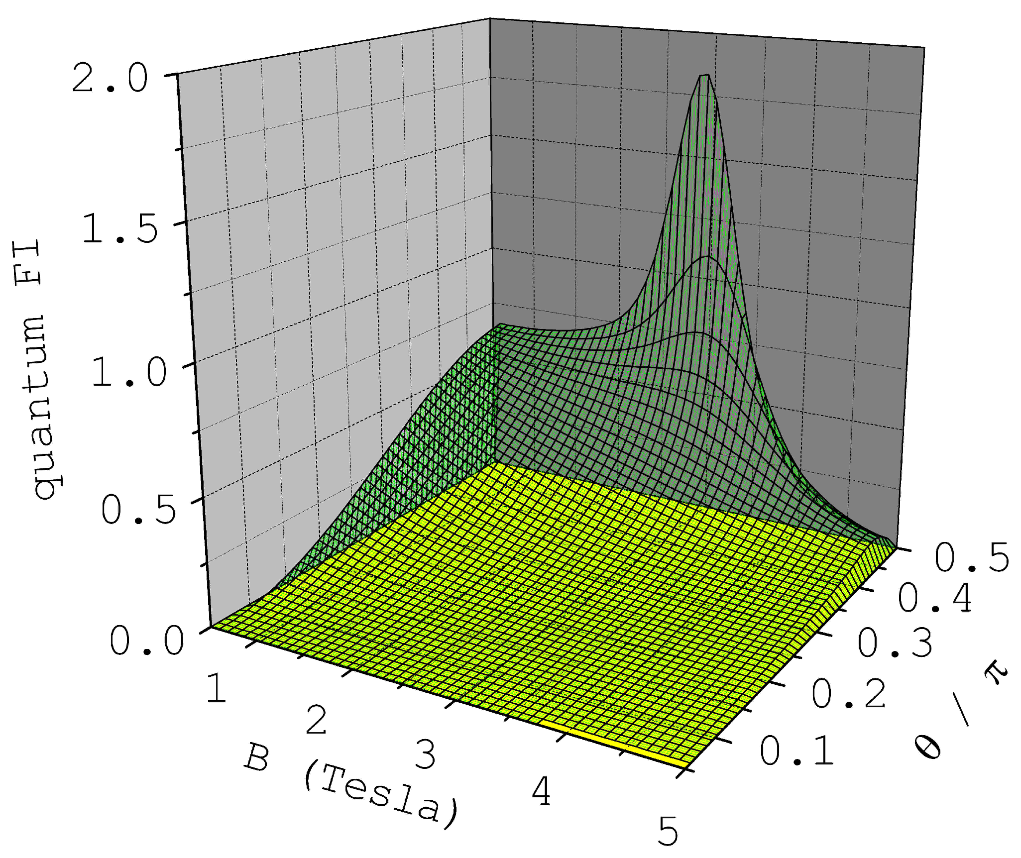
The ground state $|{\psi }_{\lambda }\rangle$ of the above Hamiltonian carries a dependence on the modulus of the applied field, which can be exploited in order to estimate $\lambda =B$ through the measurement of a suitable observable. If the observable is optimal, the highest precision in the estimation of the field is given by the QFI of $|{\psi }_{\lambda }\rangle$. The QFI of the ground state $|{\psi }_B\rangle$ is reported in Figure 1 as a function of the field intensity B and of its orientation θ, relative to the molecule easy axis (z). We note that, on average, the dependence of the ground state on B (and thus $H\left({\psi }_B\right)$) increases with the angle θ. In addition, a clear peak emerges for $\theta \simeq \pi /2$ and $B\simeq 2.5\text{T}$, in correspondence with an avoided level crossing between the ground and an excited state. This is thus the range of magnetic field values and orientations where the Fe${}_4$ molecule represents a more sensitive probe of the magnetic field.

More generally, the QFI can be used to devise the observable which is most suited for estimation of a given unknown parameter λ, which can coincide with the coupling constant, an external field, or the temperature, to mention just a few possibilities. It also allows one to determine to what extent the parameter dependence of the system state is reflected in the reduced state of a given subsystem, such as a bunch of spins within a large spin cluster. In this case, one can define a reduced QFI, which quantifies the suitability for estimating the parameter λ of measurements performed locally within the subsystem [16].

2.2.2. Quantifying the Size of Schrödinger Cat States

A Schrödinger cat state is given by the linear superposition of two diametrically opposed conditions of a physical system, such as a cat being alive and dead. While the two states are classical-like, their coexistence in the linear superpositions leads to highly nonclassical (i.e., quantum) features, as the paradoxical example of the dead and alive cat illustrates. These quantum features can be captured and quantified (amongst other means [17,18,19,20,21]) by the QFI, associated with a specific dependence of a quantum state on the parameter λ, namely $|{\psi }_{\lambda }\rangle =e^{-i\lambda X}|{\psi }_0\rangle$. One can show that the QFI of the above state simply coincides—up to a prefactor 4—with the variance of the operator X in $|{\psi }_{\lambda }\rangle$ (or, equivalently, in $|{\psi }_0\rangle$):

$$H_X\left({\psi }_{\lambda }\right)=4\left(\langle {\psi }_{\lambda }|X^2|{\psi }_{\lambda }\rangle -\langle {\psi }_{\lambda }\left|X\right|{\psi }_{\lambda }{\rangle }^2\right)=4\mathrm{Var}\left(X\right)=H_X\left({\psi }_0\right).$$

(8)

This expression of the QFI can be used to quantify the size of a Schrödinger cat state

$$|{\psi }_{SC}\rangle =\frac{1}{\sqrt{2}}(|{\psi }_1\rangle +|{\psi }_2\rangle ),$$

(9)

by setting $|{\psi }_{\lambda }\rangle =|{\psi }_{SC}\rangle$ and maximizing $H_X$ over the one-body operators X: $H\left({\psi }_{\lambda }\right)={max}_X{H}_X\left({\psi }_{\lambda }\right)$. Here $X={\sum }_{i=1}^N{\widehat{\mathbf{z}}}_i·{\mathbf{s}}_i$ is a sum of single-spin components along directions specified by the versors ${\widehat{\mathbf{z}}}_i$. The optimal operator X corresponds to the N versors ${\widehat{\mathbf{z}}}_i$ that maximize $H_X$ for the quantum state in question. It can be shown that, for a cluster formed by N spins $s_i$, the theoretical maximum of H is given by $4{({\sum }_{i=1}^N{s}_i)}^2$. Therefore, the more $H\left({\psi }_{SC}\right)$ approaches such a theoretical maximum, the more $|{\psi }_{SC}\rangle$ can be regarded as a good example of a Schrödinger cat state for that particular spin cluster. The idea underlying the use of the QFI in this context is that these highly nonclassical states can evolve very rapidly under the effect of a one-body operator [22]. As discussed in the following, such use can also be understood differently in the case of a spin cluster. In fact, the clearest example of a Schrödinger cat state in a cluster of N spins of length s is given by the linear superposition of the two states that are maximally polarized along a given direction; for example, z:

$$|{\psi }_{SC1}\rangle =\frac{1}{\sqrt{2}}(|s,\cdots ,s\rangle +|-s,\cdots ,-s\rangle ),$$

(10)

where the quantum numbers specify the projection along the quantization axis of the single-spin operators ${\mathbf{s}}_i$. The state $|{\psi }_{SC1}\rangle$ maximizes the quantum fluctuations of the operator $S_z$, with Var$\left(S_z\right)={\left(Ns\right)}^2$. The total spin projection instead represents a well-defined quantity in each of the two components $|{\psi }_1\rangle$ and $|{\psi }_2\rangle$ of the linear superposition. This can be clearly generalized to the non-collinear case,

$$|{\psi }_{SC2}\rangle =\frac{1}{\sqrt{2}}(|m_{z_1}=s,\cdots ,m_{z_N}=s\rangle +|m_{z_1}=-s,\cdots ,m_{z_N}=-s\rangle ),$$

(11)

where the z axes are now defined locally and can in principle point in different directions. Just like $|{\psi }_{SC1}\rangle$, the state $|{\psi }_{SC2}\rangle$ matches the definition of a Schrödinger cat state, which can be identified with a linear superposition of two classical-like and macroscopically distinguishable states. The components of the above linear superposition are classical-like (for they are given by the product of single-spin coherent states) and are macroscopically distinguishable (for they correspond to the largest and opposite eigenvalues of a non-collinear magnetization). The state $|{\psi }_{SC2}\rangle$ maximizes the fluctuations of the operator $X={\sum }_{i=1}^N{\widehat{\mathbf{z}}}_i·{\mathbf{s}}_i,$ being $\mathrm{Var}\left(X\right)={\left(Ns\right)}^2$. It is thus intuitive that one can use the variance of some non-collinear magnetization X as a measure of the state catness, where the versors ${\widehat{\mathbf{z}}}_i$ (and thus, X) are determined by maximizing the variance of X for the state in question. The QFI H thus represents a general theoretical tool which allows one to compare the size of different cat-like quantum states prepared in a given molecular nanomagnet (see below), and also in different molecules [23].

We consider hereafter linear superpositions between pairs of eigenstates belonging to the ground $S=5$ multiplet of the Fe${}_4$ molecule. One can show that—in the case of linear superpositions between any two states with $|\Delta M|>2$—the optimal operator X is given by the difference between the spin projections of the two sublattices: $X=s_{1,z}-{\sum }_{i=2}^4{s}_{i,z}$. In Figure 2, we report the values of the QFI for such linear superpositions (Equation 9) as a function of the total spin projections $M_1$ and $M_2$ of the states $|{\psi }_1\rangle$ and $|{\psi }_2\rangle$. From the plot it emerges that the catness of $|{\psi }_{SC}\rangle$ essentially depends on $|M_1-M_2|$ and is an increasing function of that quantity. In particular, for $M_1=-M_2=\pm 5$, one obtains values of the QFI of the same order of the theoretical maximum, which in this case is 400. We also note that, for all the considered linear superpositions, the QFI is much larger than the one obtained by simply setting $X=S_z$, being in that case $H_{S_z}={(M_1-M_2)}^2$. This comparison shows how the QFI allows one to go beyond simpler quantities that might be used in order to characterize a Schrödinger cat state in a molecular spin cluster, such as the difference between the total spin projections $|M_1-M_2|$, and also the length of the total spin S, or the number N of spins that form the cluster. In fact, unlike all of these simpler alternatives, the QFI—through the optimization of X—fully takes into account the specific nonclassical features of the spin-cluster states $|{\psi }_1\rangle$ and $|{\psi }_2\rangle$, which can also be encoded in quantum numbers other than S and M.

The application of the QFI to the characterization of states that resemble prototypical cat states (such as $|{\psi }_{SC2}\rangle$) is rather straightforward. Things become less straightforward for more general linear superpositions, where the components $|{\psi }_1\rangle$ and $|{\psi }_2\rangle$ exhibit themselves as nonclassical features. In this case, one can obtain high values of the QFI (i.e., a large amount of quantum fluctuations for one-body operators), not only in the linear superposition of two eigenstates, but also in the eigenstates themselves. In order to factor out such contributions, one can normalize the QFI of $|{\psi }_{SC}\rangle$ to that of $|{\psi }_1\rangle$ and $|{\psi }_2\rangle$. 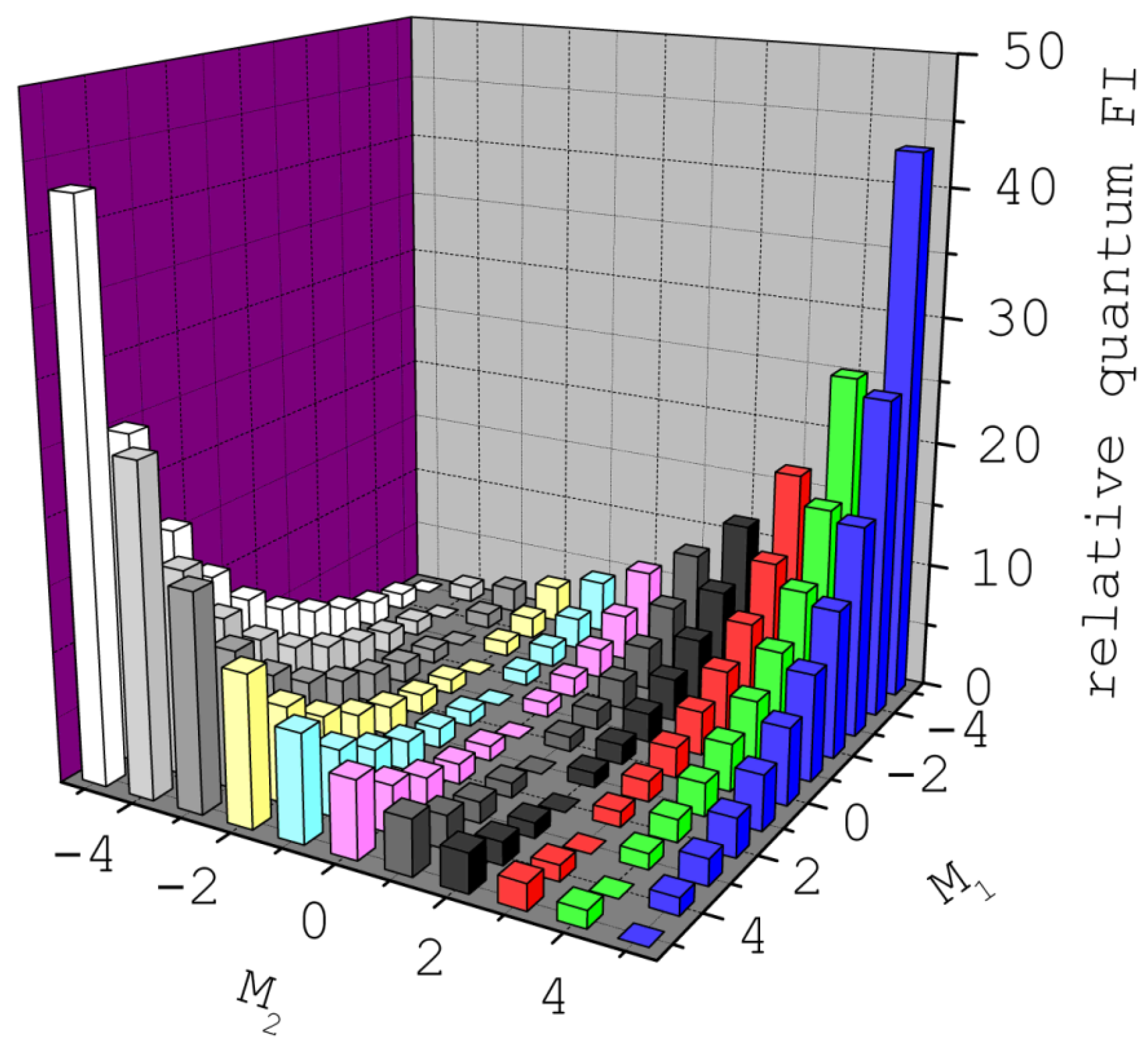This defines the relative Fisher information:

$$H_r\left({\psi }_{SC}\right)=\frac{H\left({\psi }_{SC}\right)}{\frac{1}{2}\left[H\left({\psi }_1\right)+H\left({\psi }_2\right)\right]}.$$

(12)

In Figure 3, we report the values of $H_r$ for the same set of states considered in the previous figure. Interestingly, the relative Fisher information corresponds to the ratio between the QFI of the linear superposition between $|{\psi }_1\rangle$ and $|{\psi }_2\rangle$ and that of the mixture. Therefore, $H_r$ quantifies the loss of nonclassicality which results from a dephasing process, after a linear superposition between two eigenstates has been generated: the larger $H_r$ is, the more significant is the reduction of the QFI induced by dephasing. If applied to low-spin molecules with highly-entangled ground states, the calculation of the relative Fisher information leads to the conclusion that linear superpositions of their ground states are in fact rather poor examples of Schrödinger cat states. Broadly speaking, these are systems with highly nonclassical ground states, but the degree of nonclassicality—as quantified by the quantum fluctuations of X—is not significantly enhanced by linearly superimposing the ground states [23].

As a final remark, we would like to mention a possible connection between the QFI of a linear superposition of two eigenstates, $|{\psi }_1\rangle$ and $|{\psi }_2\rangle$, and the transitions $|{\psi }_1\rangle ⟶|{\psi }_2\rangle$ induced by electron paramagnetic resonance (EPR). This connection stems from the fact that pulsed EPR is one of the most powerful ways to generate these linear superpositions. On the other hand, there seems to be a trade-off between the oscillator strength of a transition and the QFI of the corresponding linear superposition. In fact, linear superpositions generated through dipole-allowed transitions tend to have low values of $H_r$, whereas linear superpositions with large values of $H_r$ tend to correspond to forbidden transitions with $|M_1-M_2|>1$. A good compromise between the amplitude of a transition and the macroscopicity of the quantum state that this allows one to generate can be achieved close to level anticrossings, where the eigenstates exhibit strong fluctuations of the total spin projection [24].

In conclusion, we have discussed the use of the classical and quantum Fisher information in the context of molecular magnetism. In particular, we have shown that the specific heat can be regarded (up to a prefactor) as the FI of an observable corresponding to the system Hamiltonian. The QFI can be used both in parameter estimation and for quantification of the degree of nonclassicality of a quantum state. Examples of both applications were provided for the Fe${}_4$ molecular nanomagnet. In the former case, one can identify the range of magnetic field intensities and orientations where the molecule can be used as a sensitive probe of the field. In the latter case, an estimate of the catness is provided for all linear superpositions between pairs of eigenstates belonging to the ground multiplet of Fe${}_4$.

References

1. Gatteschi, D.; Sessoli, R.; Villain, J. Molecular Nanomagnets; Oxford University Press: Oxford, UK, 2007. [Google Scholar]
2. Nielsen, M.A.; Chuang, I.L. Quantum Computation and Quantum Information; Cambridge University Press: Cambridge, UK, 2010. [Google Scholar]
3. Leuenberger, M.; Loss, D. Quantum computing in molecular magnets. Nature 2001, 410, 789–793. [Google Scholar] [CrossRef] [PubMed]
4. Troiani, F.; Ghirri, A.; Affronte, M.; Carretta, S.; Santini, P.; Amoretti, G.; Piligkos, S.; Timco, G.; Winpenny, R.E.P. Molecular engineering of antiferromagnetic rings for quantum computation. Phys. Rev. Lett. 2005, 94, 207208. [Google Scholar] [CrossRef] [PubMed]
5. Lehmann, J.; Gaita-Arino, A.; Coronado, E.; Loss, D. Spin qubits with electrically gated polyoxometalate molecules. Nat. Nanotechnol. 2007, 2, 312–317. [Google Scholar] [CrossRef] [PubMed]
6. Luis, F.; Repolles, A.; Martinez-Perez, M.J.; Aguila, D.; Roubeau, O.; Zueco, D.; Alonso, P.J.; Evangelisti, M.; Camon, A.; Sese, J.; et al. Molecular prototypes for spin-based CNOT and SWAP quantum gates. Phys. Rev. Lett. 2011, 107, 117203. [Google Scholar] [CrossRef] [PubMed]
7. Siloi, I.; Troiani, F. Towards the chemical tuning of entanglement in molecular nanomagnets. Phys. Rev. B 2012, 86, 224404. [Google Scholar] [CrossRef]
8. Helstrom, C.W. Quantum Detection and Estimation Theory; Academic Press: New York, NY, USA, 1976. [Google Scholar]
9. Holevo, A.S. Statistical Structure of Quantum Theory; Springer: Berlin, Germany, 2001. [Google Scholar]
10. Thomas, L.; Lionti, F.; Ballou, R.; Gatteschi, D.; Sessoli, R.; Barbara, B. Macroscopic quantum tunneling of magnetization in a single crystal of nanomagnets. Nature 1996, 383, 145–147. [Google Scholar] [CrossRef]
11. Friedman, J.R.; Sarachik, M.P.; Tejada, J.; Ziolo, R. Macroscopic Measurement of Resonant Magnetization Tunneling in High-Spin Molecules. Phys. Rev. Lett. 1996, 76, 3830–3833. [Google Scholar] [CrossRef] [PubMed]
12. Chiolero, A.; Loss, D. Macroscopic Quantum Coherence in Molecular Magnets. Phys. Rev. Lett. 1998, 80, 169. [Google Scholar] [CrossRef]
13. Santini, P.; Carretta, S.; Amoretti, G.; Guidi, T.; Caciuffo, R.; Caneschi, A.; Rovai, D.; Qiu, Y.; Copley, J.R.D. Spin dynamics and tunneling of the Néel vector in the Fe10 magnetic wheel. Phys. Rev. B 2005, 71, 184405. [Google Scholar] [CrossRef]
14. Waldmann, O.; Stamatatos, T.C.; Christou, G.; Güdel, H.U.; Sheikin, I.; Mutka, H. Quantum Phase Interference and Néel-Vector Tunneling in Antiferromagnetic Molecular Wheels. Phys. Rev. Lett. 2009, 102, 157202. [Google Scholar] [CrossRef] [PubMed]
15. Schlegel, C.; van Slageren, J.; Manoli, M.; Brechin, E.K.; Dressel, M. Direct observation of quantum coherence in single-molecule magnets. Phys. Rev. Lett. 2008, 101, 147203. [Google Scholar] [CrossRef] [PubMed]
16. Troiani, F.; Paris, M.G.A. Probing molecular spin clusters by local measurements. 2016; arXiv:1604.06539v1. [Google Scholar]
17. Leggett, A.J. Macroscopic quantum systems and the quantum theory of measurement. Prog. Theor. Phys. Suppl. 1980, 69, 80–100. [Google Scholar] [CrossRef]
18. Dür, W.; Christoph, S.; Cirac, J.I. Effective Size of Certain Macroscopic Quantum Superpositions. Phys. Rev. Lett. 2002, 89, 210402. [Google Scholar] [CrossRef] [PubMed]
19. Shimizu, A.; Miyadera, T. Stability of Quantum States of Finite Macroscopic Systems against Classical Noises, Perturbations from Environments, and Local Measurements. Phys. Rev. Lett. 2002, 89, 270403. [Google Scholar] [CrossRef] [PubMed]
20. Björk, G.; Mana, P.G.L. A size criterion for macroscopic superposition states. J. Opt. B Quantum Semiclass. Opt. 2004, 6, 429–436. [Google Scholar] [CrossRef]
21. Marquardt, F.; Abel, B.; von Delft, J. Measuring the size of a quantum superposition of many-body states. Phys. Rev. A 2008, 78, 012109. [Google Scholar] [CrossRef]
22. Fröwis, F.; Dür, W. Size of linear superpositions in molecular nanomagnets. New J. Phys. 2012, 14, 093039. [Google Scholar] [CrossRef]
23. Troiani, F.; Zanardi, P. Size of linear superpositions in molecular nanomagnets. Phys. Rev. B 2013, 88, 094413. [Google Scholar] [CrossRef]
24. Chen, Y.; Ashkezari, M.D.; Collet, C.A.; Allao Cassaro, R.A.; Troiani, F.; Lahti, P.M.; Friedman, J.R. Observation of tunneling-assisted highly forbidden single-photon transitions in a Ni4 single-molecule magnet. 2015; arXiv:1510.03109v2. [Google Scholar]
Figure 1. Quantum Fisher information (QFI) H of the Fe 4 ground state. Here H quantifies the rate of variation of the ground state with the modulus of the applied magnetic field B, for different angles θ between B and the easy axis of the molecule. The axial anisotropy and the isotropic g factor used in the calculations are given by D = 50 μ eV and g = 2 , respectively.
Magnetochemistry 02 00033 g001
Figure 2. Quantum Fisher information corresponding to linear superpositions | ψ S C = ( | ψ 1 + | ψ 2 ) / 2 between eigenstates of the Fe 4 nanomagnet belonging to the ground S = 5 multiplet. The QFI is plotted as a function of the total spin projections M 1 and M 2 of the eigenstates | ψ 1 and | ψ 2 and quantifies the size of the linear superposition as a Schrödinger cat state.
Magnetochemistry 02 00033 g002
Figure 3. Relative quantum Fisher information corresponding to linear superpositions | ψ S C = ( | ψ 1 + | ψ 2 ) / 2 between eigenstates of the Fe 4 nanomagnet belonging to the ground S = 5 multiplet. The relative QFI is plotted as a function of the total spin projections M 1 and M 2 and corresponds to the degree of nonclassicality of the linear superposition of | ψ 1 and | ψ 2 , normalized to that of the mixture.
Magnetochemistry 02 00033 g003