End-User Software for Efficient Sensor Placement in Jacketed Wine Tanks


1
Department of Modeling and Systems Analysis, Hochschule Geisenheim University, Von-Lade-Straße 1, 65366 Geisenheim, Germany
2
Department of Enology, Hochschule Geisenheim University, Von-Lade-Straße 1, 65366 Geisenheim, Germany
*
Author to whom correspondence should be addressed.
Fermentation 2018, 4(2), 42; https://doi.org/10.3390/fermentation4020042
Submission received: 24 May 2018
/
Revised: 4 June 2018
/
Accepted: 6 June 2018
/
Published: 9 June 2018
(This article belongs to the Special Issue Wine Fermentation)
Abstract
:In food processing, temperature is a key parameter affecting product quality and energy consumption. The efficiency of temperature control depends on the data provided by sensors installed in the production device. In the wine industry, temperature sensor placement inside the tanks is usually predetermined by the tank manufacturers. Winemakers rely on these measurements and configure their temperature control accordingly, not knowing whether the monitored values really represent the wine’s bulk temperature. To address this problem, we developed an end-user software which 1. allows winemakers or tank manufacturers to identify optimal sensor locations for customizable tank geometries and 2. allows for comparisons between actual and optimal sensor placements. The analysis is based on numerical simulations of a user-defined cooling scenario. Case studies involving two different tanks showed good agreement between experimental data and simulations. Implemented based on the scientific Linux operating system gmlinux, the application solely relies on open-source software that is available free of charge.
1. Introduction
Temperature is an important factor in various processing steps during wine making [1]. Prior to fermentation, for example, a speed-up of must clarification by particle sedimentation can be achieved by appropriate tank cooling. During fermentation, temperature control allows the winemaker to define the aromatic profile of the wine and to prevent stuck or sluggish fermentations [2,3,4,5,6]. Other process steps involving temperature control are cold stabilization, malolactic fermentation or storage (aging) [1,7,8,9,10]. During active fermentation, a homogeneous temperature in the tank is achieved by efficient bubble mixing, while in processes where mixing is driven entirely by natural convection, temperature gradients in the tank are more likely [11,12,13,14,15,16].
To monitor wine temperatures, tanks are usually equipped with a single temperature sensor which is beneficial not only in terms of costs, but also regarding issues of hygienic design and clean-in-place installations. Usually, tank manufacturers do not reveal any details of their strategies and considerations behind the placement of that single sensor.
According to one manufacturer, for tanks with diameters in the range of 0.82 m to 3.6 m, winemaker’s may choose from a few different positions along the tank wall in combination with one or two different distances from the wall.
Cooling applications for wine tanks include various types of double jackets as well as plates or coils that can be immersed into the wine as required. Typically, modern tanks are equipped with a pillow plate double jacket and can be ordered fully insulated [1,17]. For these tank types, it is a common practice to keep some distance between the sensor and the tank wall where sensor values might be biased by the double-jacket cooling.
Effective temperature control is important for wine quality, e.g., by hindering evaporative losses or degradation of aromatic compounds triggered by inappropriate temperatures during storage or aging, but it is also important in terms of overall energy costs since ill-positioned sensors indicating too high bulk temperatures may obviously lead to unnecessarily high cooling loads. In fact, heating and cooling applications have been identified as the main contributors to the energy costs of industrial winerys [8,18,19,20,21,22].
Recent studies on sensors in winemaking focus on developing smart monitoring systems in the fields of wireless sensor networks and Internet of Things (IoT) not covering the topic where temperature probes should be located [23,24,25,26,27,28]. Hence, this study aims on addressing the question on efficient sensor placement in winemaking for the first time.
Considering the broad range of available tank geometries and possible sensor positions, any experiment-based optimal sensor placement is obviously inefficient and infeasible. Hence, a procedure based on numerical simulations and computational fluid dynamics (CFD) is suggested in this study. The approach was implemented into an end-user software which offers practitioners a tool for the analysis of their specific configurations. It is limited to scenarios where the tank is filled with a liquid phase only, as scenarios with a large amount of particular matter, e.g., red wine mash, would need a different modeling approach.
2. Materials and Methods
2.1. Mathematical Model
To identify suitable temperature sensor locations inside wine fermentation tanks, the software computes simulations of cooling scenarios. Before and after fermentation, the flow is assumed to be driven by natural convection only. Density variations caused by typical wine cooling conditions are assumed small, s.t. the Boussinesq approximation can be used [1,29]. Under these assumptions, numerical simulations can be performed using the buoyantBoussinesqPimpleFoam solver of the open-source C++-CFD-toolbox OpenFOAM® [30].The underlying model describes single phase flow of an incompressible fluid where density variations are only accounted for in the buoyancy term following the Boussinesq approach.
Balance Equations
Assuming laminar flow, Refs. [31,32] the following system of partial differential equations for mass (Equation (1)), momentum (Equation (2)) and energy is applicable (Equation (3)):
with , p, , , , T and Pr representing velocity (m s−1), pressure (Pa), density (kg m−3), Boussinesq gravity (m s−2), kinematic viscosity (m2 s−1), temperature (K) and Prandtl number (-). The Prandtl number is calculated as with the specific heat capacity (J kg−1 K−1).
Applying Boussinesq’s approximation, the gravity term is expressed as
with the thermal expansion coefficient (K−1) and gravity (m s−2).
2.2. Software Implementation
The end-user software is based on open-source software packages, including R (v.3.4.0) [33], Shiny by RStudio (v.1.0.3) [34], Salome (v.7.8.0) [35], OpenFOAM® (v.4.1) [30] and ParaView (v.5.0.1) [36]. To facilitate its use, it was implemented based on the scientific Linux operating system gmlinux (v.17.01) [37,38], which is an extended version of Ubuntu 16.04 LTS that provides all necessary programs pre-installed and pre-configured.Additional R packages—ggplot2 (v.2.2.1.9000) [39], Cairo (v.1.5-9) [40] and future (v.1.5.0) [41]—are installed automatically when launching the application for the first time.Computer intensive calculations such as meshing and numerical simulation are automatically run in parallel on all but one of the available processor cores. This ensures quick results while maintaining the system’s operability.
The graphical user interface is based on Shiny. It is divided into two main panels. On the left panel, data input is realized using sliders thematically distributed over four tabs, Tank, Cooling, Wine and Simulation. More details on the content of these tabs are given in Section 2.3. The right panel is used for the output of responsive graphics and texts such as tank geometry sketches or information on the expected cooling rate. A progress bar is shown when the analysis is ran in the background. In case of invalid input, data warning messages are displayed. A screenshot of the user interface is shown in Figure 1.
2.3. Case Definition
The case setup in the software environment is organized in three steps requiring user input. In the first step, geometry data of the tank, dimensions of the cooling jacket and a fill level must be supplied. This includes tank diameter (m), total tank height (m), cone angle (°), liquid volume V (m3), sediment fraction (m3 m−3), cooling jacket distance from tank height (m) and jacket height (m). In the second step, temperature conditions and cooling power of the scenario are defined. Here, the initial liquid temperature (°C) and the cooling power (W) are required. In the case of non-insulated tanks, the heat flow rate from ambient air to the liquid, (W), can also be set. To support user input, the expected cooling rate is calculated on the fly by Equation (5) and printed out in the right panel.
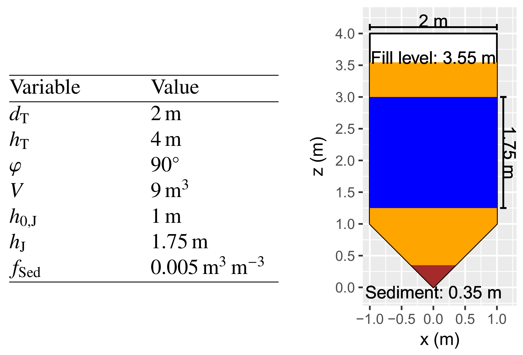
Thermo-physical properties of the liquid can be modified as required. Default values refer to a typical white wine after fermentation and are given in Table 1.
In the last step, model parameters relating to the optimal sensor placement procedure are defined. This includes simulation time (s), e.g., the length of a cooling cycle, the measurement interval of the temperature sensor (s), the accepted temperature tolerance , e.g., the sensor’s measurement tolerance, and the minimum percentage of valid measurements q (%). The simulation setup also allows for a choice of grid cell size (mm) which can be used for a trade-off between level of uncertainty and computational costs. If required, input data from previous analyses can be read from a file. Further details on the use of the input parameters and on the simulation setup are provided in the following sections.
2.4. Geometry and Mesh Generation
The software visualizes the geometrical parameters provided by the user as a 2D-sketch of the tank including fill level and sediment volume. This is useful for a fine-tuning of geometrical parameters until they match real life situations such as truncated cone bottoms. Although the current implementation supports cylindro-conical tanks only, it can also be used to approximate dished bottoms as explained in Section 2.7. Figure 2 shows the default geometrical input data and the corresponding output sketch.
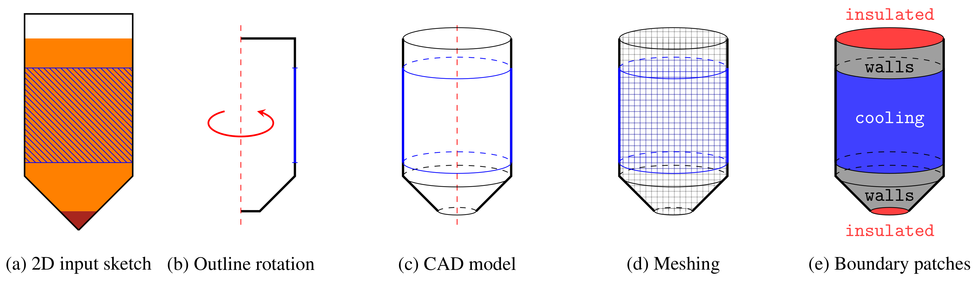
The software encompasses a fully automated mesh generation procedure (Figure 3) solely based on the geometrical input parameters and the grid cell size set by the user. Using a Python script, these data are used to generate a CAD-Model in Salome. This is realized using a rotational geometry approach referring to the outline of the fluid region of the tank as well as on information on cooling jacket position. The resulting STL-surfaces already represent the boundary patches used for the simulation setup as explained in Section 2.5. Finally, the snappyHexMesh utility of OpenFOAM® is used to built a hexahedral-dominant mesh, starting with an underlying blockMesh that uses the previously defined grid cell size .
2.5. Boundary Conditions
The computational mesh is divided into three groups of boundary patches referred to as walls, cooling and insulated (Figure 3).The walls patches represent all tank surfaces in contact with liquid and ambiance where the specified heat flow is applied. This excludes the tank bottom where sediment is assumed to insulate the fluid from ambiance, and the liquid surface where insulation caused by the air in the tank’s headspace is assumed. These regions are treated as a part of the insulated patch where a zero gradient Neumann-type boundary conditions is applied for temperature. The cooling patch corresponds to the jacketed tank surface. To express rates of heat flow () from the cooling jacket or from ambient air, Neumann-type boundary condition are applied. Boundary face values are evaluated using
where (K) is the current cell center temperature and (m) is the face-to-cell distance.
The local reference temperature gradient is calculated from the rate of heat flow as follows:
where and describe the boundary patch area (m2) and the effective thermal diffusivity (m2 s−1). Effective thermal diffusivity is calculated according to
which simplifies to
since is assumed.
A no-slip Dirichlet-type boundary conditions is applied for the velocity on all patches. Pressure is handled by OpenFOAM®’s fixedFluxPressure boundary condition, which acts similar to a zero gradient Neumann-type boundary condition including adjustments for body forces like gravity [42].
2.6. Identification of Sensor Locations
The sensor location algorithm identifies locations where a temperature sensor would most likely report the current liquid’s bulk temperature (K), ideally at all times. To guide the algorithm, the user is allowed to choose a threshold for acceptable temperature deviations, a measurement interval and a percentage of valid measurements; this can e.g., be used to better represent practical situations or the requirements discussed in Section 2.3. Based on the input data for these three constraints, most reliable temperature sensor locations are determined as follows. Each grid cell center is used as a potential sensor location. The user-defined measurement interval and overall simulation duration define the total number of sensor evaluations. To evaluate the sensor in a particular grid cell center, the deviation of the cell’s temperature from the bulk mean temperature is determined and compared to the user-defined temperature threshold . The overall percentage of valid measurements is calculated for every cell according to
with the Heaviside step function defined as:
All grid cells exceeding the user-defined threshold value q that defines the desired minimum percentage of valid measurements are classified as reliable sensor locations. An automated 3D ParaView visualization procedure is used to display the recommended sensor location cells along with a sketch of the tank geometry.
2.7. Case Studies
A proof of concept study was performed to evaluate the effectiveness and robustness of the sensor location algorithm. Two independent experiments were carried out to compare the software’s simulation results with measured temperature profiles referring to wine tank cooling. Please note that the validity of the numerical solver buoyantBoussinesqPimpleFoam has already been proven elsewhere [43,44]. Insulated wine tanks equipped with a pillow plate cooling jacket were filled with an appropriate amount of tap water. After a 24 h resting period, initial bulk temperature was determined. Then, coolant was pumped through the cooling jacket for 1 h while monitoring the liquid’s temperature at six different locations. At the end of this cooling cycle, the tank’s content was homogenized using a mechanical mixer which resulted in a homogeneous, final bulk temperature. The difference between initial and final bulk temperatures was used to compute the cooling power required in the computer simulation of the experiment.
This experiment was carried out twice using two different-sized dished bottom wine tanks, both fully insulated and equipped with pillow plate cooling jackets. Both tanks were placed on load cells to measure the tanks’ contents. The smaller tank had a diameter of dT,S = 0.6 m and was filled with 300 kg of water, the larger tank (dT,L = 1.4 m) was filled with 5420 kg. Temperature measurements were realized through thermowells on three different heights and two different depths using external probe temperature sensors (TSN-EXT44, AREXX Engineering, Zwolle, NL). With an accuracy of ±0.5 °C to ±1 °C on an operating temperature range from −30 °C to 80 °C, these sensors are similar to standard built-in wine tank sensors. The two sensors depths, measured as distances from the tank wall, for the small and the large tank were 5.5 cm/13 cm and 21 cm/34 cm, respectively. Details on the different measurement heights and tank dimensions are given in Figure 4. In the following, the six sensor locations are referred to as T-N, T-F, C-N, C-F, B-N and B-F, where T, C and B define the heights (top, center, bottom) and wall distance is expressed as N and F (near, far).
We measured an initial bulk temperature () of 13.4 °C for the large, 18.2 °C for the small tank. Final bulk temperatures were 12.92 °C in the large tank ( = 0.48 °C), and 16.88 °C in the small tank ( = 1.32 °C). This includes a correction for the rate of heat flow introduced by the mechanical mixer (TS-V17 movable mixer, 0.75 kW, 1400 rpm—Theo & Klaus Schneider GmbH & Co KG, Bretzenheim, Germany) of 405 W. Hence, for the large tank the applied cooling power () was calculated to be −3045 W from
with = 4180 J kg−1 K−1 and tc = 3600 s. In the experiment with the small tank, the cooling power was −460 W.
These experiments were then simulated in the software environment using the input data shown in Table 2. The values for kinematic viscosity, thermal expansion and thermal conductivity were taken from literature and set to = 1.5 × 10⁻⁶ m2 s−1, = 207 × 10−6 K−1 and = 0.56 W m−1 K−1 [45,46]. In addition to the standard software procedure, the simulation data was probed at the experimental sensor positions to gather temperature progressions curves similar to the experimental setup. To account for temperature variations in rotationally symmetric positions, radial mean temperatures were computed from the simulation results for each sensor position.
3. Results and Discussion
3.1. Case Studies
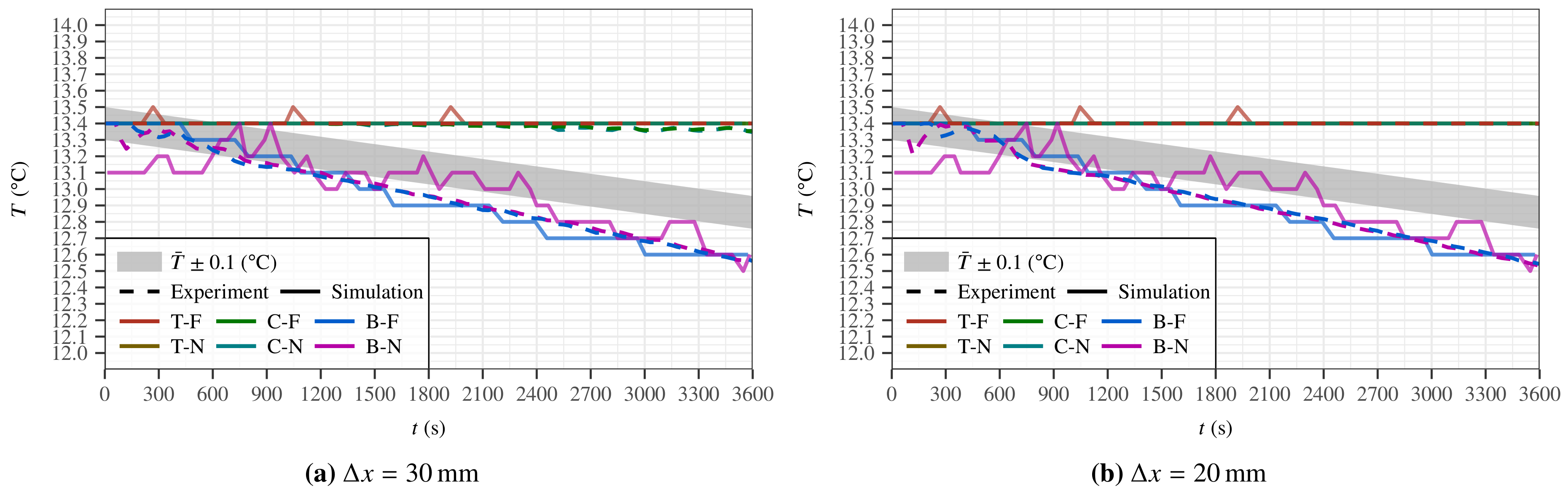
In the case studies, experimental temperature curves obtained at six different locations during a cooling cycle of 1 h were compared with simulation results. Initially, sensor data were calibrated to match initial bulk temperature. An exception was made for the B-N sensor in the large tank since its data showed inconsistencies during the first minutes. Its initial value was adjusted to represent a more physical temperature development.
In the large tank, only the lower region represented by sensors B-F and B-N was affected during 1 h of cooling (Figure 5), which can be explained by the fact that the cooling jacket was deeply immersed below the water surface (1.41 m). Minor differences in the temperature curves reported by B-F and B-B are within the range of sensor data fluctuations and thus insignificant. All remaining sensors including those located slightly above the cooling jacket (C-F, C-N) did not measure any cooling effect.
These results could be reproduced in simulations based on the end-user software and parameter settings described above. Two different grid resolutions, Δx = 30 mm and 20 mm, were used and gave similar results. A small cooling effect was detected in the simulations at sensor positions C-F and C-N, starting after approx. 30 min. Since this effect was smaller than the sensors tolerance limit, it was not observed in the experiments. We also noted that the temperature drop was more pronounced in the coarser grid case which indicates artificial numerical diffusion effects [29]. As Figure 5 shows, none of the large tank sensor locations under investigation was suitable to monitor the liquid’s bulk temperature based on a ±0.1 °C tolerance level.
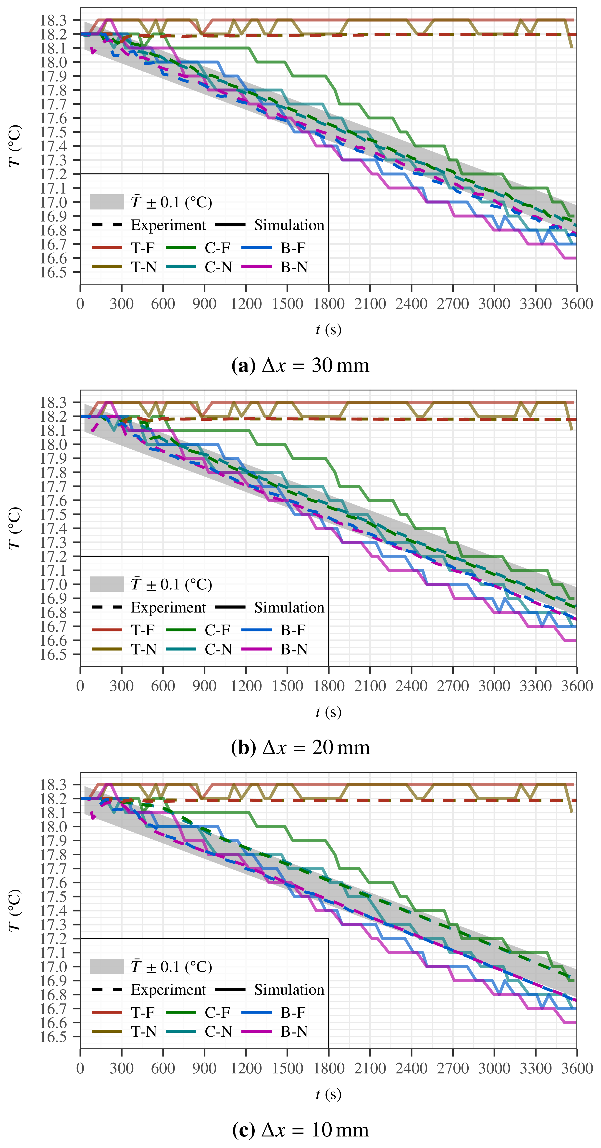
In the second case study with the smaller tank, the cooling jacket was located approximately 8 cm below the liquid surface. Similar to the large tank results, the sensors above the cooling jacket (T-F and T-N) did not detect a temperature drop during 1 h of cooling (Figure 6). All four sensors below the cooling jacket reported a steady temperature decrease while slightly lower temperatures were found closer to the tank bottom (sensors B-F and B-N). This corresponds to a typical natural convection flow pattern where cold fluid with higher density accumulates at the bottom. For the smaller tank, experimental data were compared with simulations on three different grid resolutions Δx: 30 mm, 20 mm and 10 mm. A good coincidence between simulations and experiments was found for all grid resolutions (Figure 6). Refining the grid resulted in a slightly larger temperature difference between the two lower sensor levels C-F/N and B-F/N without affecting the general cooling pattern.
The simulation results indicated that sensor positions C-F and C-N seemed preferable to monitor average bulk temperature. This will be further investigated in the following section where the consequences of different settings of the accepted percentage of valid measurements (q) and the temperature tolerance () will be compared.
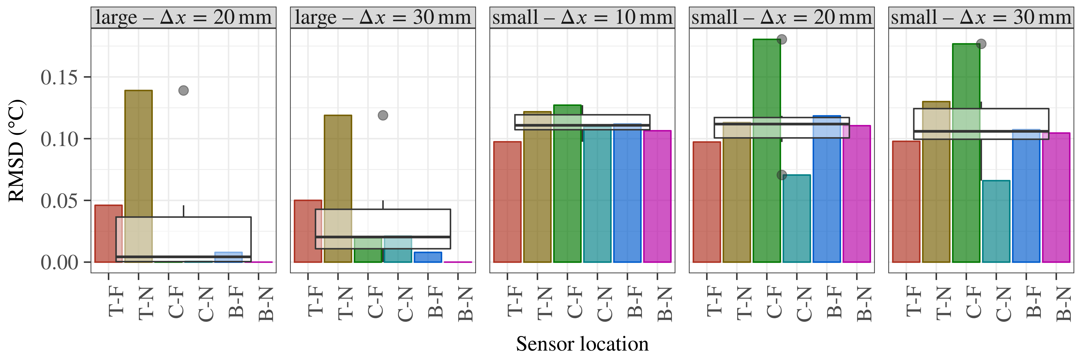
To assess grid sensitivity, the root-mean-square deviation (RMSD) between experiment and simulation was computed for all six sensor locations according to
for . Figure 7 confirms the generally good coincidence between simulations and measurements that was already evident from Figure 5 and Figure 6. While the mean RMSD in the large tank decreased with a finer grid resolution, it remained almost constant in the small tank, which, on the other hand, showed a decrease in its standard deviation as the grid was refined. This indicates a systematic difference between simulations and experiments related with fluctuations of the experimental sensor data. For example, in the temperature measurements of T-F and T-N in Figure 6, a fluctuation between 18.2 °C and 18.3 °C was present during the entire cooling cycle. Also, it must be noted that the higher RMSD accuracy for the large tank scenario is clearly related to the fact that significant cooling effects showed up at only two of the six sensors compared to four of six positions in the small tank experiment. As explained, this is a consequence of the differences in the relative positions between cooling jacket and sensors. Again, this underlines the importance to consider the individual conditions in a winery when deciding on temperature sensor locations.
3.2. Sensor Location Scenarios
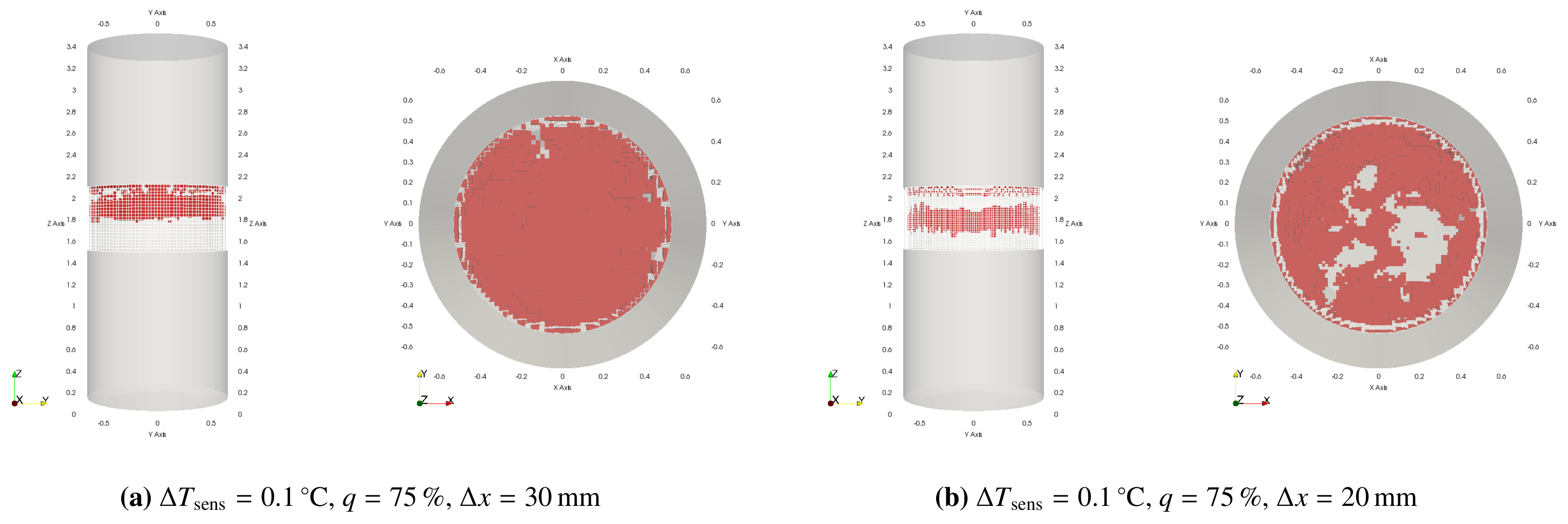
Finally, we analyze the software’s suggestions on suitable sensor locations for the two case studies. In the large tank scenario—with the cooling jacket located deeply below the water surface—the software identifies a region of suitable sensor locations that lies slightly below the upper edge of the cooling jacket (Figure 8), based onsensor parameters = 0.1 °C and q = 75%. On the finer grid, the region of suitable sensor locations is set a little lower compared to the coarser grid. Also, the finer grid suggests that a location in the central region of the tank might be less suitable compared to a location closer, but not too close, to the tank wall. From the coarser grid, on the other hand, no recommendations can be derived regarding the depth of suitable sensor locations, apart from the fact that the first few centimeters away from the cooling jacket are excluded. This corresponds to common practice where a minimum distance from the cooling jacket is always kept to avoid undesired measurement biases. Generally, it must be noted that in the large tank scenario the location of the cooling jacket is far from ideal w.r.t. temperature homogeneity. As experiments and the simulation in the previous section have shown, this configuration led to a distinct temperature stratification inside the tank which means that the use of mechanical mixers would be advisable.
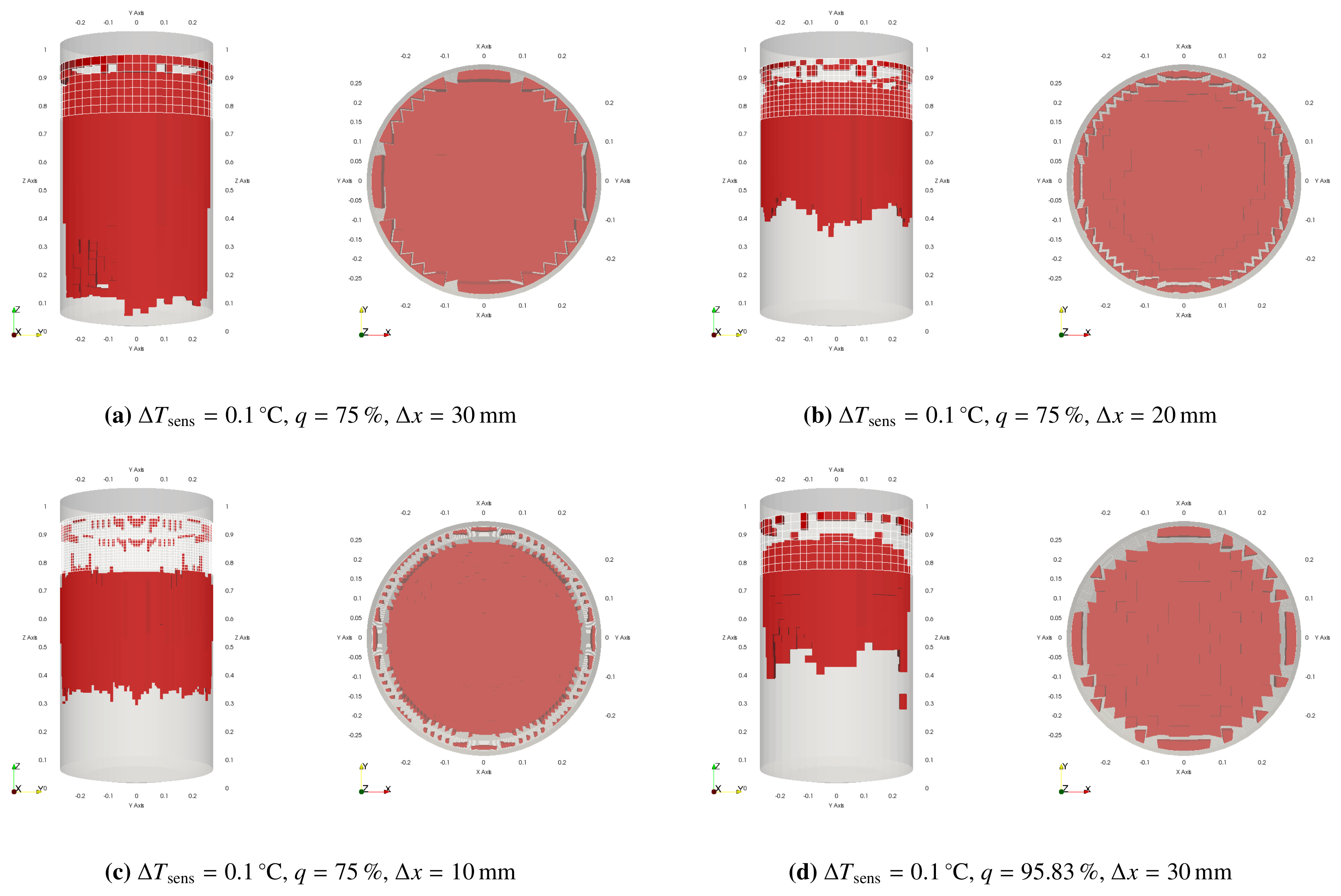
Less stratification was found in the small tank case study where the cooling jacket was located just slightly below the liquid surface. In this scenario, the differences between the regions of suitable sensor locations suggested by the software for each of the three grid resolutions were more pronounced, based on threshold parameters = 0.1 °C and q = 75% (Figure 9a–c). The results for the coarsest grid (Figure 9a, Δx = 30 mm) only excluded small portions at the bottom and top ot the tank from the suggested region of suitable sensor locations. The finer grids (Δx = 10 mm and 20 mm) identified the region of suitable sensor locations with more precision in a smaller volume, corresponding to about 1/3 to 2/3 of the liquids fill level. The larger size of the region of suitable sensor locations in comparison to the large tank scenario can be explained by the more homogeneous temperature distribution in the small tank. As discussed before, the grid refinements led to a more distinct temperature gradient between the two lower sensor levels which shrinks the size of the region of suitable sensor locations on the two finer grids relative to the coarsest grid.
By adjusting the threshold for the percentage of valid measurements to q = 95.83% (115/120 measurements) in the coarsest grid case, it was possible to shrink the region to a similar volume that was found in the simulations with the finer grid. This adjustment can be done in the post-processing step in ParaView, and hence the end-user can analyze effects of more strict thresholds after the simulation step to obtain smaller and more informative regions of suitable sensor locations. While results similar to the more computationally expensive fine grid simulations could be obtained on the coarse grid in this particular case, the end-user should be aware of the danger that the loss in accuracy on coarser grids may lead to unphysical results in other cases. The case studies suggest grid resolutions in a range between 10 mm to 30 mm for small to medium sized wine tanks as a reasonable compromise between computational costs and accuracy.
3.3. Computational Costs
Table 3 shows the computational costs for the case study simulations referring to an affordable standard workstation. As can be seen, computational times range between minutes to less than a day (1207 min), which means that it is feasible to perform the simulations with the software on standard end-user equipment, especially when choosing coarser grid resolutions. As it was shown, coarser grid simulations may already lead to a sufficiently good agreement with experimental data, while undesired effects of numerical diffusion can be reduced by lowering the threshold values. To avoid a too high loss in accuracy on coarser grids, a grid sensitivity study is recommended for tank sizes beyond the scope of this study, which can be easily realized in the end-user software by performing iterated simulations with several values.
3.4. Summary of Results
A summary of our main results is given in Table 4.
4. Conclusions
An end-user software was developed that identifies optimized sensor locations for liquid bulk temperature measurement. Based on a few input parameters, different scenarios can be analyzed and optimized, or the suitability of pre-installed sensors can be evaluated. As it was shown, ideal temperature sensor locations in wine tanks depend strongly on the fill level relative to the location of the cooling device. Since the optimized sensor positions in our case studies showed a higher variability in height compared to depth (i.e. wall distance), an enhanced mobility of the sensors in height direction would be a useful enhancement for the wine industry. In this way, effective adaptive cooling strategies could be implemented based on the software that would be sensitive to variable conditions between the years, such as yield differences. The software could be used to compute optimal sensor height from live data, with subsequent adjustments of the physical sensors that would improve process control and efficiency. Based on a parameter study across a broad range of possible scenarios, the results could be formulated in terms of more general, phenomenological mathematical approaches such as Pareto models that would allow for a faster prediction of unevaluated scenarios [47,48]. This data base could also be used for a faster identification of a range of cooling scenarios that are appropriate for pre-installed, non-movable sensors.
Author Contributions
Conceptualization, D.S., M.F. and K.V.; Data curation, D.S.; Formal analysis, D.S. and K.V.; Funding acquisition, K.V.; Investigation, D.S. and M.F.; Methodology, D.S., M.F. and K.V.; Project administration, K.V.; Resources, D.S. and M.F.; Software, D.S.; Supervision, K.V.; Validation, D.S., M.F. and K.V.; Visualization, D.S.; Writing—original draft, D.S. and K.V.; Writing—review & editing, D.S., M.F. and K.V.
Funding
This research was funded by the German Federal Ministry of Education and Research (BMBF, Germany)—grant number 05M13RNA—as a part of the joint project “Robust energy optimization of fermentation processes for the production of biogas and wine (ROENOBIO)”.
Conflicts of Interest
The authors declare no conflict of interest.
Abbreviations
The following abbreviations are used in this manuscript:
| specific heat capacity (J kg−1 K−1) | |
| tank diameter (m) | |
| sediment fraction (m3 m−3) | |
| gravitational acceleration (m s−2) | |
| Boussinesq gravity (m s−2) | |
| jacket height (m) | |
| cooling jacket distance from tank height (m) | |
| tank height (m) | |
| p | pressure (Pa) |
| Pr | Prandtl number (-) |
| turbulent Prandtl number (-) | |
| Rate of heat flow from ambient air to the liquid (W) | |
| cooling power (W) | |
| rate of heat flow (W) | |
| q | percentage of valid measurements (%) |
| T | temperature (K) |
| cell center temperature (K) | |
| cooling rate (°C h−1) | |
| accepted temperature tolerance (mm) | |
| boundary face temperature (K) | |
| initial fluid temperature (°C) | |
| local reference temperature gradient (K) | |
| reference temperature (K) | |
| measurement interval of the temperature sensor (s) | |
| simulation duration (s) | |
| velocity (m s−1) | |
| V | liquid volume (m3) |
| grid cell size (mm) | |
| Greek symbols | |
| thermal expansion coefficient (K−1) | |
| face-to-cell distance (m) | |
| thermal conductivity (W m−1 K−1) | |
| kinematic viscosity (m2 s−1) | |
| turbulent kinematic viscosity (m2 s−1) | |
| cone angle (°) | |
| density (kg m−3) | |
| Subscripts | |
| c | linear cooling |
| f | linear face |
| L | linear large tank |
| S | linear small tank |
| x | linear cell |
| Acronyms | |
| CFD | computational fluid dynamics |
References
- Boulton, R.; Singleton, V.; Bisson, L.; Kunkee, R. Heating and Cooling Applications. In Principles and Practices of Winemaking; Springer: New York, NY, USA, 1999; pp. 492–520. [Google Scholar] [CrossRef]
- Molina, A.; Swiegers, J.; Varela, C.; Pretorius, I.; Agosin, E. Influence of wine fermentation temperature on the synthesis of yeast-derived volatile aroma compounds. Appl. Microbiol. Biotechnol. 2007, 77, 675–687. [Google Scholar] [CrossRef] [PubMed]
- Masneuf-Pomarède, I.; Mansour, C.; Murat, M.L.; Tominaga, T.; Dubourdieu, D. Influence of fermentation temperature on volatile thiols concentrations in Sauvignon blanc wines. Int. J. Food Microbiol. 2006, 108, 385–390. [Google Scholar] [CrossRef] [PubMed]
- Beltran, G.; Novo, M.; Guillamón, J.M.; Mas, A.; Rozès, N. Effect of fermentation temperature and culture media on the yeast lipid composition and wine volatile compounds. Int. J. Food Microbiol. 2008, 121, 169–177. [Google Scholar] [CrossRef] [PubMed]
- Torija, M.; Rozès, N.; Poblet, M.; Guillamón, J.M.; Mas, A. Effects of fermentation temperature on the strain population of Saccharomyces cerevisiae. Int. J. Food Microbiol. 2003, 80, 47–53. [Google Scholar] [CrossRef] [Green Version]
- Bisson, L.F. Stuck and Sluggish Fermentations. Am. J. Enol. Vitic. 1999, 50, 107–119. [Google Scholar]
- Benitez, J.G.; Macias, V.P.; Gorostiaga, P.S.; Lopez, R.V.; Rodriguez, L.P. Comparison of electrodialysis and cold treatment on an industrial scale for tartrate stabilization of sherry wines. J. Food Eng. 2003, 58, 373–378. [Google Scholar] [CrossRef]
- Jourdes, M.; Michel, J.; Saucier, C.; Quideau, S.; Teissedre, P.L. Identification, amounts, and kinetics of extraction of C-glucosidic ellagitannins during wine aging in oak barrels or in stainless steel tanks with oak chips. Anal. Bioanal. Chem. 2011, 401, 1531. [Google Scholar] [CrossRef] [PubMed]
- Forsyth, K.; Roget, W.; O’Brien, V. Improving Winery Refrigeration Efficiency, Final Report, Project Number AWR 0902; The Australian Wine Research Institute: Adelaide, Australia, 2012. [Google Scholar]
- Soccol, C.R.; Pandey, A.; Larroche, C. Fermentation Processes Engineering in the Food Industry; CRC Press: Boca Raton, FL, USA, 2013. [Google Scholar]
- Schmidt, D.; Velten, K. Numerical simulation of bubble flow homogenization in industrial scale wine fermentations. Food Bioprod. Process. 2016, 100, 102–117. [Google Scholar] [CrossRef]
- Zenteno, M.I.; Pérez-Correa, J.R.; Gelmi, C.A.; Agosin, E. Modeling temperature gradients in wine fermentation tanks. J. Food Eng. 2010, 99, 40–48. [Google Scholar] [CrossRef]
- Vlassides, S.; Block, D.E. Evaluation of cell concentration profiles and mixing in unagitated wine fermentors. Am. J. Enol. Vitic. 2000, 51, 73–80. [Google Scholar]
- Han, Y.; Wang, R.; Dai, Y. Thermal stratification within the water tank. Renew. Sustain. Energy Rev. 2009, 13, 1014–1026. [Google Scholar] [CrossRef]
- Takamoto, Y.; Saito, Y. Thermal Convection in Cylindro-Conical Tanks During the Early Cooling Process. J. Inst. Brew. 2003, 109, 80–83. [Google Scholar] [CrossRef] [Green Version]
- Meironke, H.; Kasch, D.; Sieg, R. Determining the thermal flow structure inside fermenters with different shapes using Ultrasonic Doppler Velocimetry. In Proceedings of the 10th International Symposium on Ultrasonic Doppler Methods for Fluid Mechanics and Fluid Engineering, Tokyo, Japan, 28–30 September 2016; pp. 125–128. [Google Scholar]
- Schandelmaier, B. Gärsteuerung 2013—Ob groß oder klein—Pillow plates müssen sein. Das Dtsch. Weinmagazin 2013, 20, 30–36. [Google Scholar]
- Morakul, S.; Mouret, J.R.; Nicolle, P.; Trelea, I.C.; Sablayrolles, J.M.; Athes, V. Modelling of the gas–liquid partitioning of aroma compounds during wine alcoholic fermentation and prediction of aroma losses. Process Biochem. 2011, 46, 1125–1131. [Google Scholar] [CrossRef] [Green Version]
- Galitzky, C.; Worrell, E.; Healy, P.; Zechiel, S. Benchmarking and self-assessment in the wine industry. In Proceedings of the 2005 ACEEE Summer Study on Energy Efficiency in Industry, West Point, NY, USA, 19–22 July 2005. [Google Scholar]
- Perez-Coello, M.; Gonzalez-Vinas, M.; Garcia-Romero, E.; Diaz-Maroto, M.; Cabezudo, M. Influence of storage temperature on the volatile compounds of young white wines. Food Control 2003, 14, 301–306. [Google Scholar] [CrossRef]
- Joyeux, A.; Lafon-Lafourcade, S.; Ribéreau-Gayon, P. Evolution of acetic acid bacteria during fermentation and storage of wine. Appl. Environ. Microbiol. 1984, 48, 153–156. [Google Scholar] [PubMed]
- Lafon-Lafourcade, S.; Carre, E.; Ribéreau-Gayon, P. Occurrence of lactic acid bacteria during the different stages of vinification and conservation of wines. Appl. Environ. Microbiol. 1983, 46, 874–880. [Google Scholar] [PubMed]
- Boquete, L.; Cambralla, R.; Rodríguez-Ascariz, J.; Miguel-Jiménez, J.; Cantos-Frontela, J.; Dongil, J. Portable system for temperature monitoring in all phases of wine production. ISA Trans. 2010, 49, 270–276. [Google Scholar] [CrossRef] [PubMed]
- Zhang, W.; Skouroumounis, G.K.; Monro, T.M.; Taylor, D. Distributed Wireless Monitoring System for Ullage and Temperature in Wine Barrels. Sensors 2015, 15, 19495–19506. [Google Scholar] [CrossRef] [PubMed] [Green Version]
- Cañete, E.; Chen, J.; Martín, C.; Rubio, B. Smart Winery: A Real-Time Monitoring System for Structural Health and Ullage in Fino Style Wine Casks. Sensors 2018, 18, 803. [Google Scholar] [CrossRef] [PubMed]
- Ranasinghe, D.C.; Falkner, N.J.; Chao, P.; Hao, W. Wireless sensing platform for remote monitoring and control of wine fermentation. In Proceedings of the 2013 IEEE Eighth International Conference on Intelligent Sensors, Sensor Networks and Information Processing, Melbourne, VIC, Australia, 2–5 April 2013; pp. 503–508. [Google Scholar]
- Sainz, B.; Antolín, J.; López-Coronado, M.; Castro, C.D. A Novel Low-Cost Sensor Prototype for Monitoring Temperature during Wine Fermentation in Tanks. Sensors 2013, 13, 2848–2861. [Google Scholar] [CrossRef] [PubMed] [Green Version]
- Di Gennaro, S.F.; Matese, A.; Mancin, M.; Primicerio, J.; Palliotti, A. An Open-Source and Low-Cost Monitoring System for Precision Enology. Sensors 2014, 14, 23388–23397. [Google Scholar] [CrossRef] [PubMed]
- Ferziger, J.H.; Peric, M. Computational Methods for Fluid Dynamics; Springer Science & Business Media: New York, NY, USA, 2012. [Google Scholar]
- Weller, H.G.; Tabor, G.; Jasak, H.; Fureby, C. A tensorial approach to computational continuum mechanics using object-oriented techniques. Comput. Phys. 1998, 12, 620–631. [Google Scholar] [CrossRef]
- Rodríguez, I.; Castro, J.; Pérez-Segarra, C.; Oliva, A. Unsteady numerical simulation of the cooling process of vertical storage tanks under laminar natural convection. Int. J. Therm. Sci. 2009, 48, 708–721. [Google Scholar] [CrossRef]
- Papanicolaou, E.; Belessiotis, V. Transient natural convection in a cylindrical enclosure at high Rayleigh numbers. Int. J. Heat Mass Trans. 2002, 45, 1425–1444. [Google Scholar] [CrossRef]
- R Core Team. R: A Language and Environment for Statistical Computing; R Foundation for Statistical Computing: Vienna, Austria, 2017. [Google Scholar]
- Chang, W.; Cheng, J.; Allaire, J.; Xie, Y.; McPherson, J. Shiny: Web Application Framework for R. R Package Version 1.0.3. 2017. Available online: https://cran.r-project.org/package=shiny (accessed on 24 May 2018).
- CEA/DEN, EDF R&D, O.C. SALOME Geometry User’s Guide. CEA/DEN, EDF R&D, OPEN CASCADE, 2016. Available online: http://docs.salome-platform.org/7/gui/GEOM/ (accessed on 24 May 2018).
- Ahrens, J.; Geveci, B.; Law, C. ParaView: An End-User Tool for Large Data Visualization; Visualization Handbook; Elsevier: Amsterdam, The Netherlands, 2005. [Google Scholar]
- Günther, M.; Velten, K. Mathematische Modellbildung und Simulation; Wiley-VCH: Berlin, Germeny, 2014. [Google Scholar]
- Velten, K.; Müller, J.; Schmidt, D. New methods to optimize wine production at all stages from vineyard to bottle. BIO Web Conf. 2015, 5, 02013. [Google Scholar] [CrossRef] [Green Version]
- Wickham, H. Ggplot2: Elegant Graphics for Data Analysis; Springer: New York, NY, USA, 2009. [Google Scholar]
- Urbanek, S.; Horner, J. Cairo: R Graphics Device Using Cairo Graphics Library for Creating High-Quality Bitmap (PNG, JPEG, TIFF), vector (PDF, SVG, PostScript) and Display (X11 and Win32) Output. R Package Version 1.5-9. 2015. Available online: https://cran.r-project.org/package=Cairo (accessed on 24 May 2018).
- Bengtsson, H. Future: Unified Parallel and Distributed Processing in R for Everyone. R Package Version 1.5.0. 2017. Available online: https://cran.r-project.org/package=future (accessed on 24 May 2018).
- Greenshields, C. OpenFOAM User Guide, v5 ed.; CFD Direct Ltd.: Reading, UK, 2017; Available online: https://cfd.direct/openfoam/user-guide/ (accessed on 24 May 2018).
- De Moura, M.D.; Júnior, A.C. Heat Transfer by Natural ConvectIon in 3D Enclosures. In Proceedings of the ENCIT 2012, Rio de Janeiro, Brazil, 18–22 November 2012. [Google Scholar]
- Corzo, S.F.; Ramajo, D.E.; Nigro, N.M. CFD model of a moderator tank for a pressure vessel PHWR nuclear power plant. Appl. Therm. Eng. 2016, 107, 975–986. [Google Scholar] [CrossRef]
- McQuillan, F.J.; Culham, J.R.; Yovanovich, M.M. Properties of Some Gases and Liquids at One Atmosphere; Technical Report; Microelectronics Heat Transfer Laboratory Report UW/MHTL 8407 G-02; Microelectronics Heat Transfer Laboratory, University of Waterloo: Waterloo, ON, Canada, 1984. [Google Scholar]
- Wagner, W.; Pruß, A. The IAPWS Formulation 1995 for the Thermodynamic Properties of Ordinary Water Substance for General and Scientific Use. J. Phys. Chem. Ref. Data 2002, 31, 387–535. [Google Scholar] [CrossRef]
- Velten, K. Mathematical Modeling and Simulation: Introduction for Scientists and Engineers; John Wiley & Sons: New York, NY, USA, 2009. [Google Scholar]
- Safikhani, H.; Hajiloo, A.; Ranjbar, M. Modeling and multi-objective optimization of cyclone separators using CFD and genetic algorithms. Comput. Chem. Eng. 2011, 35, 1064–1071. [Google Scholar] [CrossRef]
Figure 1.
Screenshot of the graphical user interface. Dashed boxes indicate the input (left) and the responsive information panel (right).
Figure 1.
Screenshot of the graphical user interface. Dashed boxes indicate the input (left) and the responsive information panel (right).
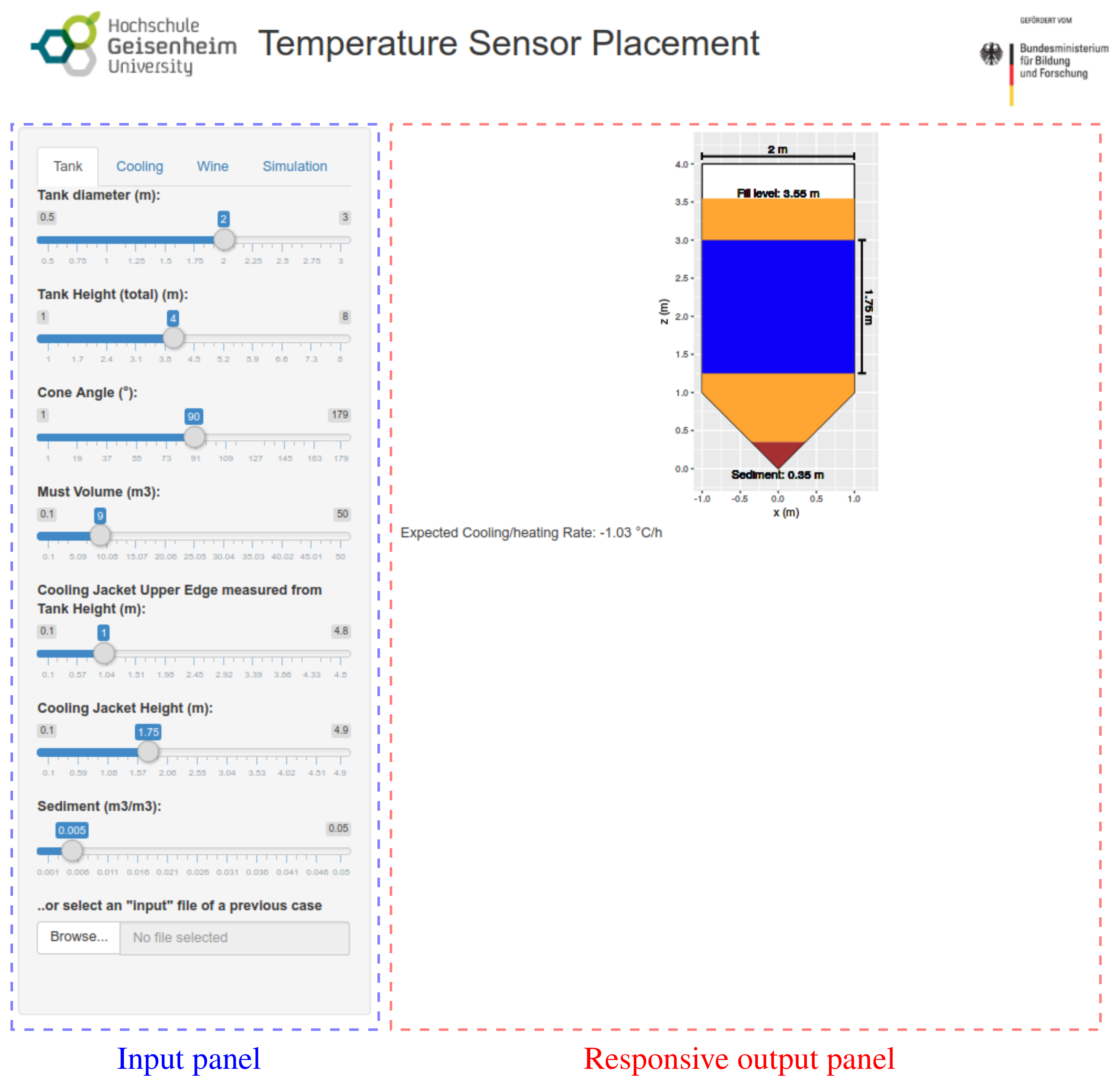
Figure 2.
Exemplary geometrical input data with corresponding 2D tank sketch.

Figure 3.
Five steps (a–e) of the fully automated mesh generation workflow.

Figure 4.
Dimensions, cooling jacket configuration and sensor locations of the (a) large and (b) small case study tank. To compare sizes the large tank and left version of the small tank are drawn on the same scale.
Figure 4.
Dimensions, cooling jacket configuration and sensor locations of the (a) large and (b) small case study tank. To compare sizes the large tank and left version of the small tank are drawn on the same scale.
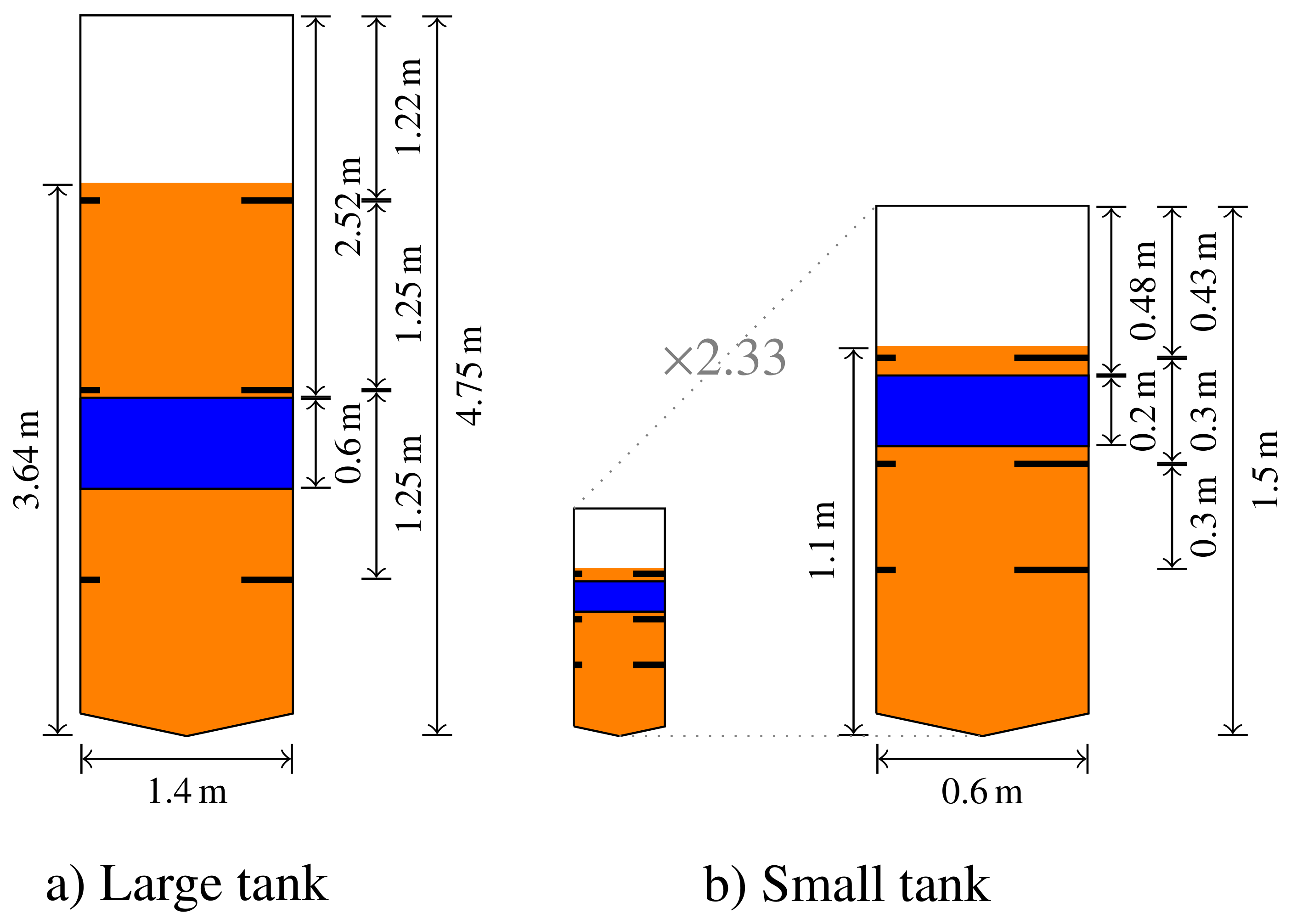
Figure 5.
Comparison of experimental cooling data in the large tank with simulations, referring to six different sensor locations inside the tank and grid cell sizes of 30 mm (a) and 20 mm (b).
Figure 5.
Comparison of experimental cooling data in the large tank with simulations, referring to six different sensor locations inside the tank and grid cell sizes of 30 mm (a) and 20 mm (b).

Figure 6.
Comparison of the experimental cooling process in the small tank with simulation data on three different grid resolutions (), 30 mm (a); 20 mm (b) and 10 mm (c), referring to six different sensor locations inside the tank.
Figure 6.
Comparison of the experimental cooling process in the small tank with simulation data on three different grid resolutions (), 30 mm (a); 20 mm (b) and 10 mm (c), referring to six different sensor locations inside the tank.

Figure 7.
Root-mean-square deviation (RMSD) of liquid temperature between measurement and simulation for each sensor location and all case studies (large/small tank on different grid resolutions ()). Box-plots represent across sensor location RMSD data for each study.
Figure 7.
Root-mean-square deviation (RMSD) of liquid temperature between measurement and simulation for each sensor location and all case studies (large/small tank on different grid resolutions ()). Box-plots represent across sensor location RMSD data for each study.

Figure 8.
Post-processing output showing suitable sensor locations (red) for the large tank case study assessed for different ((a): 30 mm; (b): 20 mm) and constant threshold values ( = 0.1 °C and q = 75%).
Figure 8.
Post-processing output showing suitable sensor locations (red) for the large tank case study assessed for different ((a): 30 mm; (b): 20 mm) and constant threshold values ( = 0.1 °C and q = 75%).

Figure 9.
Post-processing output showing suitable sensor locations (red) for the small tank case study assessed for different ((a): 30 mm; (b): 20 mm; (c): 10 mm) and constant threshold values ((a–c): = 0.1 °C and q = 75%). (d) Effect of changing the percentage of valid measurements q to 95.83% for = 30 mm.


Table 1.
Required thermo-physical properties of the liquid and their default values.
| Variable | Value |
|---|---|
| 3960 J kg−1 K−1 | |
| 970 kg m−3 | |
| 1.6 × 10⁻⁶ m2 s−1 | |
| 207 × 10−6 K−1 | |
| 0.6 W m−1 K−1 |
Table 2.
Case studies: software input data for the small and large tank geometry.
| Variable | Small Tank | Large Tank |
|---|---|---|
| 0.6 m | 1.4 m | |
| 1.5 m | 4.75 m | |
| 156° | 156° | |
| 0.3 m3 | 5.42 m3 | |
| 0.48 m | 2.52 m | |
| 0.2 m | 0.6 m | |
| 0.005 m3 m−3 | 0.005 m3 m−3 |
Table 3.
Computational costs depending on grid size in the small and large tank scenarios.
| Δx | Grid Cells | Cores a | Simulation Time (min) | ||
|---|---|---|---|---|---|
| Real Time | Single Core | ||||
| small | 30 mm | 12,805 | 3 | 3.73 | 11.19 |
| 20 mm | 40,154 | 18 | 8.92 | 160.56 | |
| 10 mm | 310,252 | 18 | 157.25 | 2830.5 | |
| large | 30 mm | 214,036 | 3 | 729.47 | 2188.4 |
| 20 mm | 714,920 | 15 | 1207.35 | 21,735.54 | |
a System: 2 × Intel®Xeon®CPU E5-2660 v3 @ 2.60GHz–64GB RAM.
Table 4.
Summary of results.
| Case studies | - Successful validation of CFD simulations against experimental temperature progression in 300 L and 5420 L jacketed wine tanks. - Pre-installed sensor locations not well suited to monitor bulk mean temperature. |
| Sensor locations | - Efficient sensor location depends on fill level and cooling jacket position. - More variability in height than in depth (distance to wall) |
| Computational costs | - Computational times of less than one day already lead to sufficient results. |
© 2018 by the authors. Licensee MDPI, Basel, Switzerland. This article is an open access article distributed under the terms and conditions of the Creative Commons Attribution (CC BY) license (http://creativecommons.org/licenses/by/4.0/).
Share and Cite
MDPI and ACS Style
Schmidt, D.; Freund, M.; Velten, K. End-User Software for Efficient Sensor Placement in Jacketed Wine Tanks. Fermentation 2018, 4, 42. https://doi.org/10.3390/fermentation4020042
AMA Style
Schmidt D, Freund M, Velten K. End-User Software for Efficient Sensor Placement in Jacketed Wine Tanks. Fermentation. 2018; 4(2):42. https://doi.org/10.3390/fermentation4020042
Chicago/Turabian StyleSchmidt, Dominik, Maximilian Freund, and Kai Velten. 2018. "End-User Software for Efficient Sensor Placement in Jacketed Wine Tanks" Fermentation 4, no. 2: 42. https://doi.org/10.3390/fermentation4020042
Note that from the first issue of 2016, this journal uses article numbers instead of page numbers. See further details here.