Dynamics of Internal Envelope Solitons in a Rotating Fluid of a Variable Depth

Abstract

We consider the dynamics of internal envelope solitons in a two-layer rotating fluid with a linearly varying bottom. It is shown that the most probable frequency of a carrier wave which constitutes the solitary wave is the frequency where the growth rate of modulation instability is maximal. An envelope solitary wave of this frequency can be described by the conventional nonlinear Schrödinger equation. A soliton solution to this equation is presented for the time-like version of the nonlinear Schrödinger equation. When such an envelope soliton enters a coastal zone where the bottom gradually linearly increases, then it experiences an adiabatical transformation. This leads to an increase in soliton amplitude, velocity, and period of a carrier wave, whereas its duration decreases. It is shown that the soliton becomes taller and narrower. At some distance it looks like a breather, a narrow non-stationary solitary wave. The dependences of the soliton parameters on the distance when it moves towards the shoaling are found from the conservation laws and analysed graphically. Estimates for the real ocean are presented.

1. Introduction

The effect of the Earth’ rotation on the dynamics of nonlinear waves in the oceans was extensively studied in the last decades (see, for example, References [1,2,3,4,5,6,7,8] and references therein). As well-know, wave propagation in big lakes can also be affected by the Earth’ rotation [9,10,11,12,13]. In particular, the dynamics of solitary waves has been investigated within the framework of the Ostrovsky equation and it was established that they cannot propagate steadily because of the permanent radiation of small-amplitude long waves [14,15] (however, they can steadily propagate being supported by a long background wave [16,17]). As a result, an initial solitary wave experiences a terminal decay which leads formally to it vanishing in a finite time [3,18]. However, the process of solitary wave decay is more complicated in reality and leads eventually to the formation of envelope solitons described by the nonlinear Shrödinger (NLS) equation or its modifications [19,20,21,22,23,24]. In an inhomogeneous medium, the dynamics of solitary waves is determined by the synergetic effects of inhomogeneity and fluid rotation. In particular, at a certain relationship between these two factors, a Korteweg–de Vries (KdV) soliton propagating towards a coast with a gradually decreasing depth can preserve its shape and amplitude, whereas its width and velocity adiabatically changes [8].

In the real ocean, when a KdV soliton approaches a coastal zone, it can experience a terminal decay in the domain where the depth is constant, so that it can be ultimately transformed into an NLS envelop soliton, and then the envelop soliton can enter into the inhomogeneous domain where an oceanic depth gradually decreases. An NLS soliton can be formed from a rather arbitrary initial perturbation independently on the transformation of a KdV soliton. It is a matter of interest to study the adiabatic dynamics of an NLS envelop soliton when it approaches a shoaling zone. To this end, we consider below different models of NLS-type equations for water waves in a rotating ocean, their solutions in the form of envelop solitons, and the dynamics of such solitons in the ocean with a gradually decreasing depth.

2. The Variable Coefficients Ostrovsky Equation

The dynamics of weakly nonlinear waves in a rotating inhomogeneous ocean can be described by the Ostrovsky equation with the variable coefficients (see, e.g., References [2,4] and the references therein):

$$\frac{\partial }{\partial x}\left(\frac{\partial u}{\partial t}+c\frac{\partial u}{\partial x}+\alpha u\frac{\partial u}{\partial x}+\beta \frac{{\partial }^{3}u}{\partial x^3}+\frac{u}{2}\frac{dc}{dx}\right)=\gamma u,$$

(1)

where for internal waves in a two-layer fluid in the Boussinesq approximation the coefficients are

$$c=\sqrt{g\frac{\delta \rho }{\rho }\frac{h_1{h}_2}{h_1+h_2}}\alpha =\frac{3}{2}c\frac{h_1-h_2}{h_1{h}_2},\beta =\frac{c}{6}{h}_1{h}_2,\gamma =\frac{f^2}{2c},$$

(2)

where $h_1=const$, and $h_2=h_2\left(x\right)$.

For the boundary-value problem, $u(t,0)=f\left(t\right)$, this equation can be presented in the alternative (“signalling”) form dubbed here the time-like Ostrovsky equation:

$$\frac{\partial }{\partial t}\left(\frac{\partial u}{\partial x}+\frac{1}{c\left(x\right)}\frac{\partial u}{\partial t}-\frac{\alpha }{c^2\left(x\right)}u\frac{\partial u}{\partial t}-\frac{\beta }{c^4\left(x\right)}\frac{{\partial }^{3}u}{\partial t^3}+\frac{u}{2c\left(x\right)}\frac{dc}{dx}\right)=-\gamma \left(x\right)u.$$

(3)

The dispersion relation corresponding to Equation (3) with the constant coefficients is

$$k\left(\omega \right)=\frac{\omega }{c}+\frac{\beta }{c^4}{\omega }^3-\frac{\gamma }{\omega }.$$

(4)

In the homogeneous non-rotating ocean, Equation (3) has a particular solution in the form of KdV soliton:

$$u(t,0)=A_K{\mathrm{sech}}^2\left(\frac{t-x/V}{{\mathsf{\Delta }}_t}\right),$$

(5)

where the soliton temporal duration ${\mathsf{\Delta }}_t$ and speed $V_K$ are related to the soliton amplitude $A_K$ through the formulae

$${\mathsf{\Delta }}_t=\frac{1}{c}\sqrt{\frac{12\beta }{\alpha A_K}},V_K=\frac{c}{1-\alpha A_K/3c}.$$

(6)

It is assumed that such a soliton in the course of propagation in a rotating ocean of a constant depth after long-term evolution will ultimately be transformed into an envelope soliton as described in References [19,20,21,22]. We assume then that the resultant envelope soliton enters into the coastal zone, where the depth gradually decreases with x. Our aim is to describe the fate of such a soliton and present the dependences of its parameters on distance.

3. The Variable Coefficients NLS Equation

In the coastal zone, where the bottom profile gradually varies with the distance, the NLS equation describing soliton evolution contains the additional “inhomogeneous” term and has the form of the “time-like NLS” (TNLS) equation (cf. References [25,26,27]):

$$i\left(\frac{\partial \psi }{\partial x}+\frac{1}{c_g\left(x\right)}\frac{\partial \psi }{\partial t}+\frac{\psi }{2}\frac{dln{c}_g}{dx}\right)+\frac{p\left(x\right)}{c_g^3\left(x\right)}\frac{{\partial }^2\psi }{\partial t^2}+\frac{q\left(x\right)}{c_g\left(x\right)}{\left|\psi \right|}^2\psi =0,$$

(7)

where the coefficients $p\left(x\right)$ and $q\left(x\right)$ are linked with the coefficients of the Ostrovsky Equation (1) (cf. Reference [22]):

$$p\left(x\right)=-c^3\left(x\right)\left[\frac{3\beta \left(x\right)}{c^4\left(x\right)}\omega -\frac{\gamma \left(x\right)}{{\omega }^3}\right],q\left(x\right)=-\frac{2}{3}\frac{{\alpha }^2\left(x\right){\omega }^{3}c\left(x\right)}{4\beta \left(x\right){\omega }^4+\gamma \left(x\right)c^4\left(x\right)}.$$

(8)

The group velocity $c_g\left(x\right)$ as follows from the Ostrovsky Equation (1) is

$$c_g\left(x\right)=c\left(x\right)-3\beta \left(x\right)k^2\left(x\right)-\frac{\gamma \left(x\right)}{k^2\left(x\right)}.$$

(9)

Note that in a stationary, but spatially inhomogeneous media, the wavenumber k depends on x, whereas the frequency is maintained.

The dependence of the wavenumber of a carrier wave on the spatial coordinate x follows from the dispersion relation Equation (4) where $\omega =const.$, and other parameters, c, $\beta$, and $\gamma$ depend on x.

Using the results obtained in Reference [22], let us present the soliton solution of the TNLS Equation (7) assuming that all its coefficients are constants:

$$\psi =A\mathrm{sech}\left[\mathsf{\Omega }\left(t-\frac{x}{c_g}-\frac{x}{V}\right)\right]e^{i\left[\sigma \left(t-x/c_g\right)-\kappa x\right]},$$

(10)

where the amplitude A and speed V can be considered as the free parameters, whereas soliton duration $\mathsf{\Delta }T=1/\mathsf{\Omega }$, $\mathsf{\Omega }=A{c}_{g0}\sqrt{q_0/2p_0}$, and the chirp and gauge respectively are:

$$\sigma =\frac{c_{g0}^3}{2p_{0}V},\kappa =\frac{q_0}{2c_{g0}}\left(\frac{c_{g0}^4}{2p_0{q}_0{V}^2}-A^2\right).$$

(11)

In the particular case when $V\to \infty$, we obtain

$$\mathsf{\Omega }=A{c}_{g0}\sqrt{\frac{q_0}{2p_0}},\sigma =0,\kappa =-\frac{q_0{A}^2}{2c_{g0}}.$$

(12)

The solution to Equation (10) is invalid when the dispersion coefficient p in the TNLS Equation (7) vanishes. This occurs at the frequency ${\omega }_{m0}=c_0\sqrt[4]{{\gamma }_0/3{\beta }_0}$ when the group velocity has a maximum ${\left(c_{g0}\right)}_{max}=c_0-2\sqrt{3{\beta }_0{\gamma }_0}$. In a such case, the generalised NLS equation derived in References [19,20] should be used.

If the envelope soliton Equation (10) enters the region where the coefficients of TNLS Equation (7) gradually varies with x, then the adiabatic evolution of the soliton’s main parameters A and V can be determined from the balance equations, which follows from the conservation laws for the TNLS equation ([28,29], see also Reference [30]). Alternatively, the rigorous asymptotic theory can be developed, but as has been shown in Reference [31], the outcome reduces to the first two conservation laws, the conservation of the total flux of “quasi-particles”:

$$N\equiv c_g\left(x\right)\underset{-\infty }{\overset{+\infty }{\int }}{\left|\psi \right|}^{2}dt=const$$

(13)

and conservation of quasi-momentum:

$$P\equiv \frac{2i}{c_g\left(x\right)}\underset{-\infty }{\overset{+\infty }{\int }}{\psi }^{*}{\psi }_{t}dt=const.$$

(14)

Substituting the soliton solution of Equation (10) into Equation (13), we obtain after simple manipulations:

$$\frac{A}{A_0}=\sqrt{\frac{p\left(x_0\right)}{p\left(x\right)}\frac{q\left(x\right)}{q\left(x_0\right)}}.$$

(15)

Then, from Equation (14), using Equation (10) and the result obtained for the soliton amplitude in Equation (15), we derive for the soliton speed:

$$\frac{A{\left(x\right)}^2\sigma }{c_g\left(x\right)}\sim \frac{A{\left(x\right)}^2{c}_g^2\left(x\right)}{V\left(x\right)p\left(x\right)}=const.$$

(16)

From here, we find:

$$\frac{V\left(x\right)}{V\left(x_0\right)}=\frac{c_g^2\left(x\right)}{c_g^2\left(x_0\right)}\frac{A^2\left(x\right)}{A^2\left(x_0\right)}\frac{p\left(x_0\right)}{p\left(x\right)}=\frac{c_g^2\left(x\right)}{c_g^2\left(x_0\right)}\frac{p^2\left(x_0\right)}{p^2\left(x\right)}\frac{q\left(x\right)}{q\left(x_0\right)}.$$

(17)

After that, we can determine the evolution of the other soliton parameters by means of the relationships (Equation (11)).

In the particular case, when $V\to \infty$ $(\sigma \to 0)$, Equation (17) vanishes, and we have only one Equation (15) determining the evolution of soliton amplitude.

As mentioned above, the TNLS Equation (7) becomes invalid when its dispersion coefficient vanishes, then the generalised NLS equation derived in References [19,20] should be used. In the next section, we consider this special case.

4. Generalised Variable Coefficients NLS Equation

In the vicinity of the point where the second-order dispersion in the TNLS equation becomes very small or vanishes, i.e., when $p\left(x\right)\to 0$, the equation should be generalised by inclusion of additional terms [19]. For the boundary-value problem, the corresponding equation reads

$$i\left({\psi }_x+\frac{1}{c_g\left(x\right)}{\psi }_t+\frac{\psi }{2}\frac{dln{c}_g}{dx}\right)+\frac{p\left(x\right)}{c_g^3\left(x\right)}{\psi }_{tt}+\frac{q\left(x\right)}{c_g\left(x\right)}{\left|\psi \right|}^2\psi -$$

$$i\frac{\nu \left(x\right)}{c_g^4\left(x\right)}{\psi }_{ttt}-\frac{i}{c_g^2}{r}_1\left(x\right)\left[{\psi }^2{\overline{\psi }}_t+r_2\left(x\right){\left|\psi \right|}^2{\psi }_t\right]=0,$$

(18)

where $\overline{\psi }$ stands for complex-conjugate with respect to function $\psi$, and the coefficients $\nu \left(x\right)$ and $r\left(x\right)$ are linked with the coefficients of the Ostrovsky Equation (1) (cf. Reference [19]):

$$\nu \left(x\right)=-\left[\beta \left(x\right)+\frac{\gamma \left(x\right)c^4\left(x\right)}{{\omega }^4}\right],$$

$$r_1\left(x\right)=\frac{2}{3}\frac{{\alpha }^2\left(x\right){\omega }^2{c}^2\left(x\right)}{4\beta \left(x\right){\omega }^4+\gamma \left(x\right)c^4},r_2\left(x\right)=\frac{4\beta \left(x\right){\omega }^4+5\gamma \left(x\right)c^4\left(x\right)}{4\beta \left(x\right){\omega }^4+\gamma \left(x\right)c^4\left(x\right)}.$$

The soliton solution to Equation (18) with the constant coefficients has the same form as Equation (10), but in contrast to the conventional NLS soliton, it is now a one parametric solution with only one independent parameter. If we choose the amplitude as the independent parameter, then other soliton parameters can be presented as follows:

$$\mathsf{\Omega }=A{c}_g\sqrt{\frac{r_1(1+r_2)}{6\nu }},\sigma =\frac{c_{g}q}{2r_1}\left[1-\frac{p{r}_1(1+r_2)}{3q\nu }\right],$$

(19)

$$V=\frac{12c_g^2\nu r_1^2}{9q^2{\nu }^2+6pq\nu r_1(1-r_2)-3p^2{r}_1^2-p^2{r}_1^2{r}_2(2-r_2)-2A^2\nu r_1^3(1+r_2)},$$

(20)

$$\kappa =\frac{-18A^2\nu (1+r_2)\left[p{r}_1(1-r_2)+3q\nu \right]+p^3\left[5+9r_2+3r_2^2-r_2^3\right]+F}{216c_g{\nu }^2},$$

(21)

$$whereF=\frac{9pq\nu }{r_1^2}\left[3q\nu \left(1-r_2\right)-p{r}_1\left(3+2r_2-r_2^2\right)\right]+27{\left(\frac{q\nu }{r_1}\right)}^3.$$

This solution can be reduced to the conventional NLS envelope soliton Equation (10) if we assume that $\nu \to 0$, $r_1\to 0$, $r_2\to 0$, but such that $r_1(1+r_2)/\nu \to 3q/p$.

In another limiting case, when $p=0$, the parameters of the soliton solution as the functions of amplitude are

$$V=\frac{12c_g^2\nu r_1^2}{\nu \left[9q^2\nu -2A^2{r}_1^3\left(1+r_2\right)\right]},\sigma =\frac{c_{g}q}{2r_1},\kappa =\frac{q\left[\nu q^2-2A^2{r}_1^3\left(1+r_2\right)\right]}{8c_g{r}_1^3},$$

(22)

and $\mathsf{\Omega }\left(A\right)$ remains the same as in Equation (19).

When a solition propagates in the inhomogeneous medium, its frequency remains constant, but the wavenumber varies in accordance with the formula (cf. Equation (4)):

$$k\left(x\right)=\frac{\omega }{c\left(x\right)}+\frac{\beta \left(x\right)}{c^4\left(x\right)}\omega -\frac{\gamma \left(x\right)}{\omega }.$$

(23)

As follows from this equation, the critical wavenumber, where the group velocity has a maximum, adiabatically changes in accordance with the variation of parameters. Therefore, if the envelope soliton has been created near the critical point, it will remain further than the corresponding critical point.

According to the numerical results of Reference [19], envelope solitons emerging from the KdV solitons in the course of long-term evolution have almost zero correction to the group speed (see Figure 9 in Reference [19]). In our notations this corresponds to $V=\infty$. Such value of speed correction corresponds to a soliton with a fixed amplitude:

$$\begin{array}{ccc}\hfill A_0& =& \sqrt{\frac{3\nu q\left[3\nu q+2p{r}_1(1-r_2)\right]-p^2{r}_1^2\left[3+r_2(2-r_2)\right]}{2\nu r_1^3(1+r_2)}}\mathrm{for}\mathrm{Equation}\left(20\right),\hfill \end{array}$$

(24)

$$\begin{array}{ccc}\hfill A_0& =& \sqrt{\frac{9\nu q^2}{2r_1^3\left(1+r_2\right)}}\mathrm{for}\mathrm{Equation}\left(22\right).\hfill \end{array}$$

(25)

The gauge $\kappa$ and parameter $\mathsf{\Omega }$ determining the half-width of a soliton are also fixed in this case:

$$\begin{array}{ccc}\hfill {\kappa }_0& =& \frac{\left[p{r}_1\left(1+r_2\right)-3q\nu \right]{\left[p{r}_1\left(2-r_2\right)+3q\nu \right]}^2}{27c_g{\nu }^2{r}_1^3}\mathrm{for}\mathrm{Equation}\left(20\right),\hfill \end{array}$$

(26)

$$\begin{array}{ccc}\hfill {\kappa }_0& =& -\frac{\nu q^3}{c_g{r}_1^3}\mathrm{for}\mathrm{Equation}\left(22\right);\hfill \end{array}$$

(27)

$$\begin{array}{ccc}\hfill {\mathsf{\Omega }}_0& =& \frac{2c_g}{r_1\nu }\sqrt{3\nu q\left[\nu q+2p{r}_1(1-r_2)\right]-p^2{r}_1^2\left[1+r_2(2-r_2)/3\right]},\mathrm{for}\mathrm{Equation}\left(20\right),\hfill \end{array}$$

(28)

$$\begin{array}{ccc}\hfill {\mathsf{\Omega }}_0& =& \frac{q{c}_g\sqrt{3}}{2r_1}\mathrm{for}\mathrm{Equation}\left(22\right).\hfill \end{array}$$

(29)

In an inhomogeneous medium, all soliton parameters from Equations (19)–(21) vary with x. The equation governing the parameter variations follows from the conservation of a total flux of “quasi-particles” as per Equation (13):

$$\frac{A\left(x\right)}{A\left(x_0\right)}=\sqrt{\frac{\nu \left(0\right)}{\nu \left(x\right)}\frac{r_1\left(x\right)\left[1+r_2\left(x\right)\right]}{r_1\left(0\right)\left[1+r_2\left(0\right)\right]}}.$$

(30)

Then, using Equations (19)–(21), one can determine variation of the parameter $\mathsf{\Omega }\left(x\right)$, velocity $V\left(x\right)$, and gauge $\kappa \left(x\right)$, whereas the chirp $\sigma \left(x\right)$ varies adiabatically as per Equation (19) and independently of soliton amplitude.

In the limiting case, when $p=0$, all soliton parameters are determined only by the coefficients of the generalised NLS Equation (18). Then, its amplitude can vary adiabatically with x only at a very special relationship between the coefficient $\alpha$ and linear wave speed c such that ${\alpha }^2\left(x\right)c\left(x\right)=const$.

5. What Is the Most Probable Frequency of Envelope Soliton?

Consider the constant coefficients of NLS Equation (7). As follows from the analysis of the stability of a uniform wave train with the amplitude amplitude $a_0$, the modulation instability occurs when $pq>0$. In our case, as follows from Equation (8), q is always positive, whereas p becomes positive when $\omega >{\omega }_{m0}$. The maximum growth rate of modulation instability is $\mathsf{\Gamma }=q{a}_0^2/c_g$ (see, e.g., References [32,33,34]). Substituting here q as per Equation (8), we obtain

$$\mathsf{\Gamma }\left(\omega \right)=\frac{2}{3}\frac{{\left(\alpha a_0\right)}^2{\omega }^3}{4\beta {\omega }^4+3\gamma c^4}.$$

(31)

This expression has a maximum at ${\omega }_{max}=c{(9\gamma /4\beta )}^{1/4}$, where the maximal growth rate for the given amplitude of a wave train is

$${\mathsf{\Gamma }}_{max}=\frac{{\left(\alpha a_0\right)}^2}{4\sqrt{6}\beta c}\sqrt[4]{\frac{\beta }{\gamma }}.$$

(32)

Thus, one can expect that an envelope soliton will evolve from a quasilinear wave train with the carrier frequency ${\omega }_{max}$ corresponding to the maximal growth rate of modulation instability. This agrees with the arguments presented in Reference [24], where it was shown that an envelope soliton cannot emerge at the carrier frequency ${\omega }_{m0}$, as was assumed in References [19,20,21], but should emerge at a higher carrier frequency. The concrete carrier frequency was not found, but only roughly estimated from the numerical data. As follows from the above theory, the relative frequency shift is fairly significant:

$$\frac{{\omega }_{max}-{\omega }_{m0}}{{\omega }_{m0}}=\sqrt[4]{\frac{27}{4}}-1\approx 0.62.$$

(33)

Therefore, one can expect that in the process of evolution of a KdV soliton in a uniform rotating ocean, it eventually transforms into an NLS envelope soliton with the carrier frequency ${\omega }_{max}$. If such a soliton enters into a coastal zone with a gradually decreasing depth, it then changes adiabatically, and its basic parameters, amplitude A and velocity V, vary with x in accordance with Equations (15) and (17).

6. Estimations for the Real Oceanic Conditions

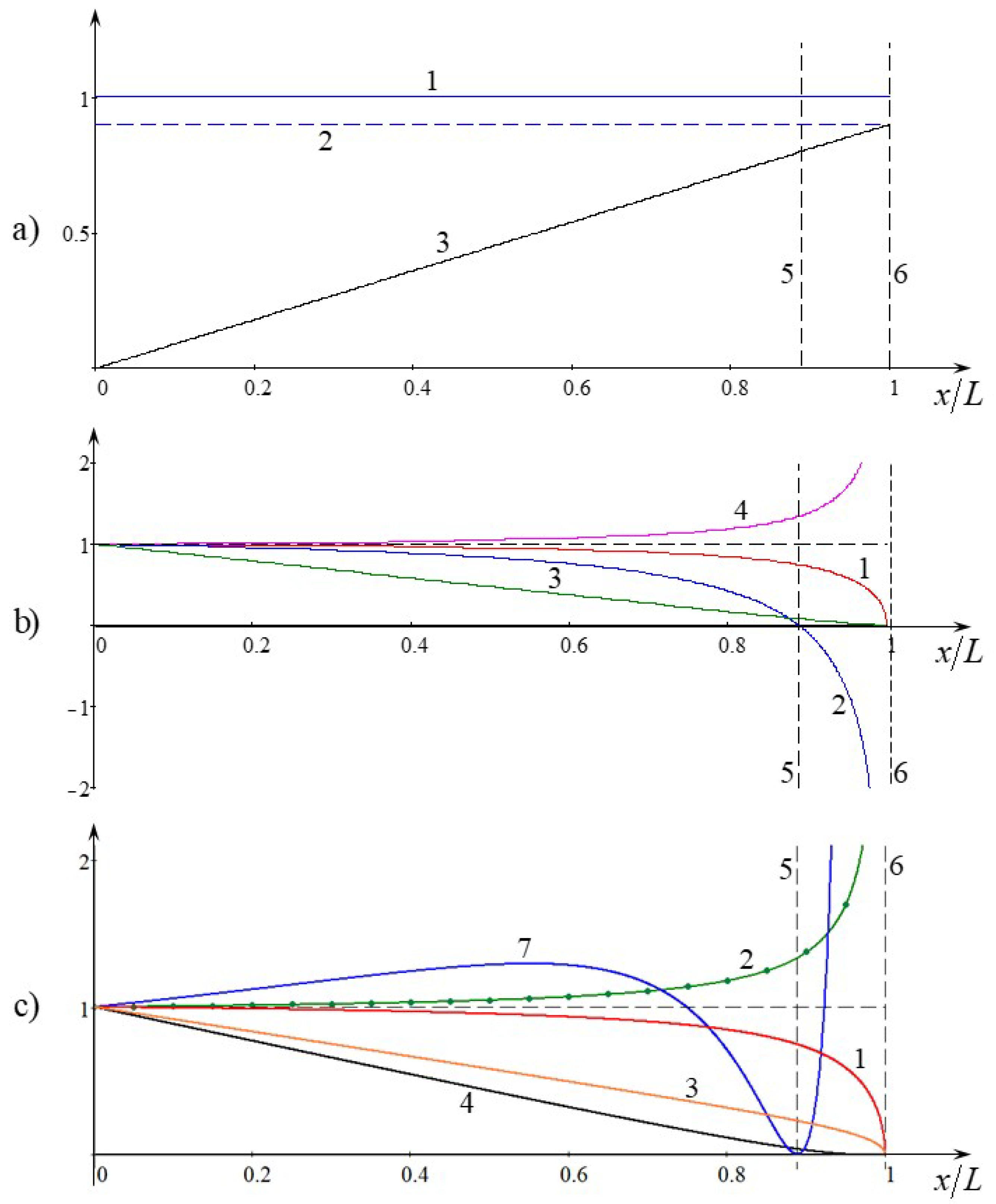
Let us assume that in the coastal zone the bottom profile is a linear function of a distance, so that the depth linearly decreases from $H_1=500$ m up to $H_2=50$ m at the distance $L={10}^6$ m, and the pycnocline is located at the depth $h_1=50$ m as shown in Figure 1a. Then, the initial thickness of the lower layer $h_2\left(0\right)=450$ m; it gradually decreases with the distance $h_2\left(x\right)=h_2\left(0\right)(1-x/L)$ and becomes zero at $x=L$. The normalised bottom profile $1-\left[h_1+h_2\left(x\right)\right]/H_1$ is shown by line 3 in Frame (a) of Figure 1. Let us set the Coriolis parameter $f={10}^{-4}$ 1/s, which is a typical value for the moderate latitudes, and $g^{\prime }\equiv g\mathsf{\Delta }\rho /\rho =0.03$ m/s${}^2$. With this parameters we obtain for the time-like Ostrovsky Equation (3) the following values of coefficients: $c=1.162$ m/c, $\alpha =-3.1\times {10}^{-2}$ 1/s, $\beta =4.36\times {10}^3$ m${}^3$/s, $\gamma =4.3\times {10}^{-9}$ 1/(m· s).

The dependences of these coefficients on the distance are shown in Figure 1b. The nonlinear coefficient $\alpha$ vanishes at some distance $x_1$, where $h_2\left(x_1\right)$ becomes equal to $h_1$. Then, it changes its sign and becomes positive. This effect is well-known (see, e.g., References [35,36] and the references therein). To avoid confusion, it should be kept in mind that the the nonlinear coefficient in this figure is presented in the normalised form $\alpha \left(x\right)/\alpha \left(0\right)$, therefore this ratio is positive when $x=0$ and becomes negative when $x_1<x<L$.

Frame (c) demonstrates the dependences of coefficients in the TNLS Equation (7). Line 1 for the normalised linear speed $c\left(x\right)$ in this frame is the same as in Frame (b), and line 3 illustrates the dependence of normalised group speed $c_g\left(x\right)$ as per Equation (9). Line 2 shows the dependence of the carrier wave number for the envelope soliton Equation (10) when $\omega ={\omega }_{max}$. This dependence is practically indistinguishable from the similar dependence plotted for $\omega ={\omega }_{m0}$; the latter one is shown in the same frame by dots on line 2. Line 4 shows the dependence of dispersion coefficient $p\left(x\right)$, and line 7 shows the dependence of nonlinear coefficient $p\left(x\right)$ as per Equation (8).

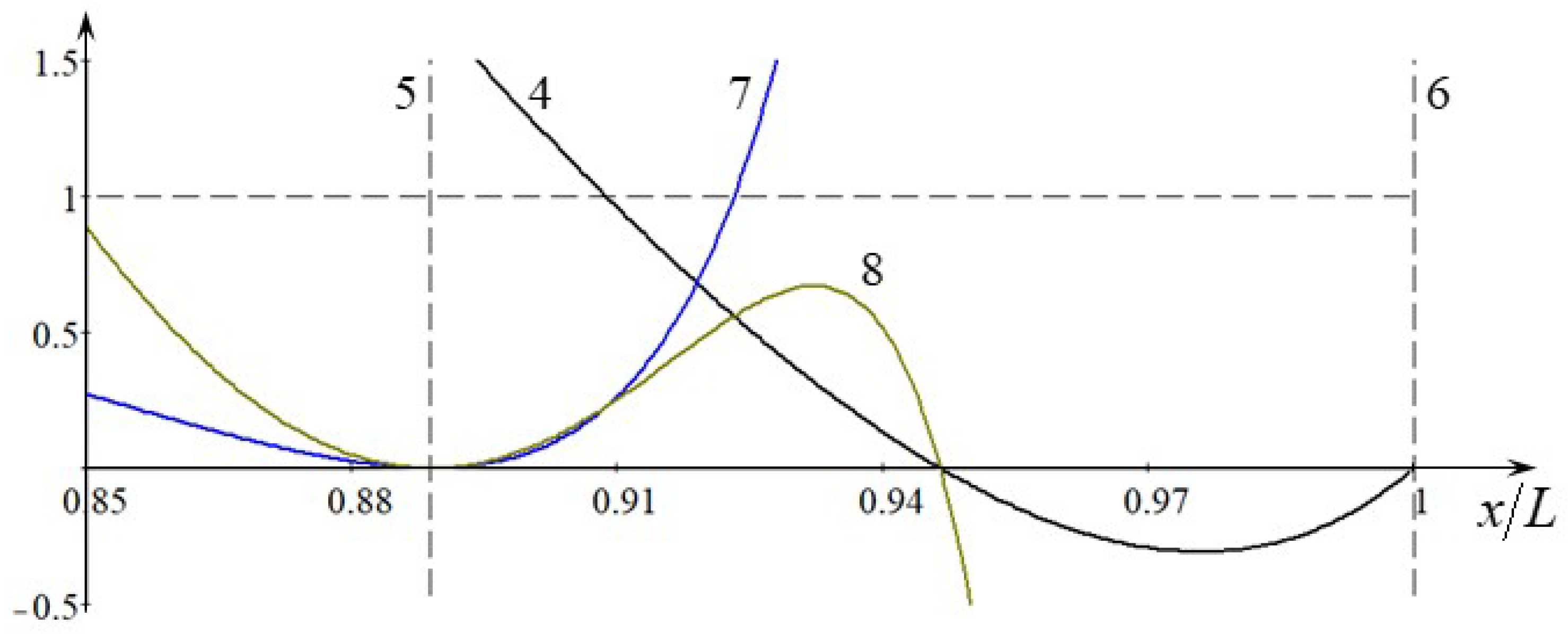
In the vicinity of distance $x=x_1\approx 0.889L$ (see vertical dashed line 5), the dispersion and nonlinear coefficients experience dramatic changes. The nonlinear coefficient q becomes zero at $x=x_1$, and then quickly increases in absolute value remaining negative for all $x\ne x_1$. The dispersion coefficient p becomes zero a bit further along, at $x_2\approx 0.947L$, and then changes its sign from negative to positive; this is shown in details in Figure 2, where the dispersion coefficient is multiplied by a factor of 50 to make it clearly visible (we remind you again that these coefficients are presented in the normalised forms in Figure 1 and Figure 2). Again in the Figure 2, a normalised product $p\left(x\right)q\left(x\right)$ (see line 8) is also shown, which determines the modulation stability/instability. The instability occurs when this product is positive (see, e.g., References [32,33,34]). In our case, the modulation instability providing the existence of NLS envelop solitons of Equation (10) occurs when either $x<x_1$ or $x_1<x<x_2$. In the vicinity of $x=x_1$ and $x=x_2$, the TNLS equation is not valid and should be replaced by the generalised NLS Equation (18).

Now, let us estimate the key parameters of the NLS envelope soliton Equation (10). A carrier frequency (where the growth rate of modulation instability has a maximum) is ${\omega }_{max}=c{(9\gamma /4\beta )}^{1/4}\approx 1.42\times {10}^{-3}$ 1/s (the corresponding period is $T_{max}\approx 4.43\times {10}^3$ s), and the maximal spatial growth rate of Equation (32) for the initial amplitude $a_0=1$ m is ${\mathsf{\Gamma }}_{max}\approx 1.94\times {10}^{-5}$ 1/m. The carrier wave number $k\left({\omega }_{max}\right)$ where the growth rate of modulation instability has a maximum is $k_m\approx 1.23\times {10}^{-3}$ 1/m (the corresponding wavelength ${\lambda }_m\approx 5.1$ km), whereas the carrier wave number $k\left({\omega }_{m0}\right)$, where the group velocity has a maximum is $k_c\approx 7.54\times {10}^{-4}$ 1/m (${\lambda }_c\approx 8.3$ km).

The nonlinear coefficient in the time-like NLS Equation (7) at $x=0$ is $q\left(k_m\right)=-2.7\times {10}^{-5}$ 1/(m${}^2·$s), and the dispersion coefficients at the same point is $p\left(k_m\right)=-13.6$ (m${}^2$/s).

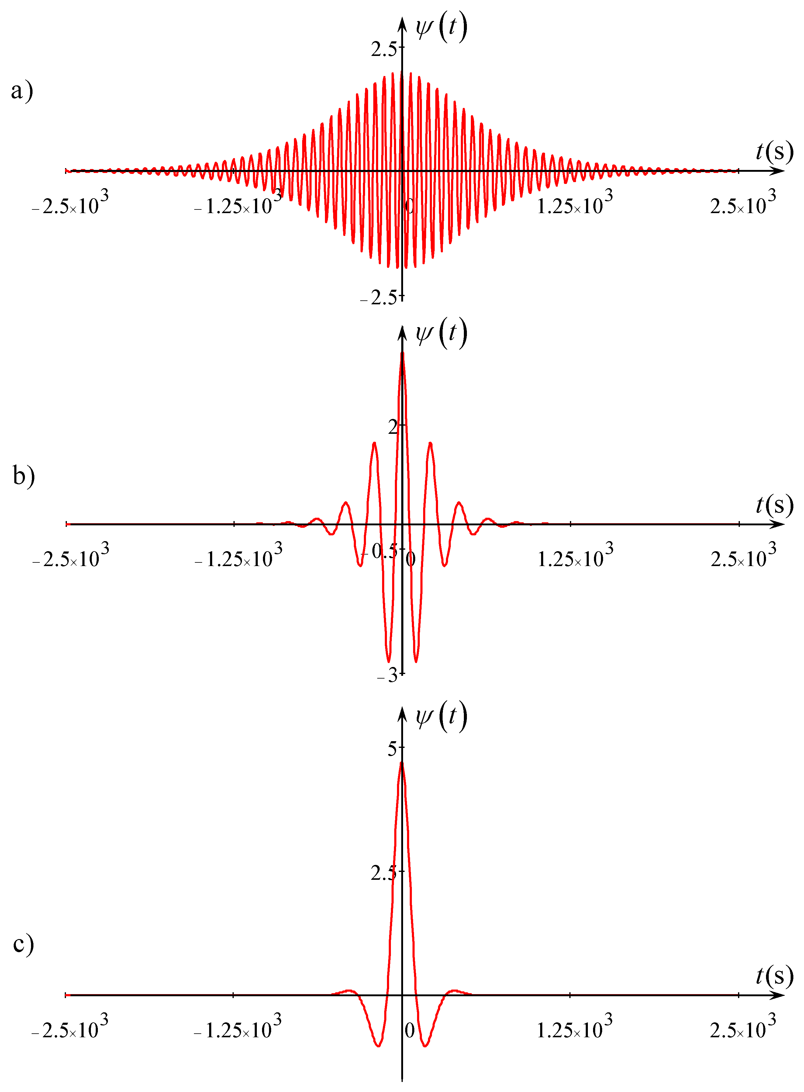
If we assume that an NLS soliton of Equation (10) has the initial amplitude $A_0=2$ m and velocity $V_0=0.5c_g\left(0\right)=0.57$ m/s, then we obtain that its characteristic duration is: $\mathsf{\Delta }T\left(0\right)\equiv 1/{\mathsf{\Omega }}_0=\sqrt{2p\left(k_m\right)/q\left(k_m\right)}/\left|A_0{c}_g\left(k_m\right)\right|\approx 440$ s $\approx 7.3$ min. The soliton chirp Equation (11) at $x=0$ is $\left|\sigma \left(0\right)\right|=c_g{\left(0\right)}^3/2\left|p\left(0\right)\right|V\left(0\right)=0.095$ 1/s and the corresponding carrier wave period is $T_c\left(0\right)\equiv 2\pi /\left|\sigma \left(0\right)\right|\approx 66$ s. This means that there are $N\left(0\right)=\mathsf{\Delta }T\left(0\right)/T_c\left(0\right)\approx 7$ carrier wave periods on the half-duration of envelope soliton (see Frame (a) in Figure 3).

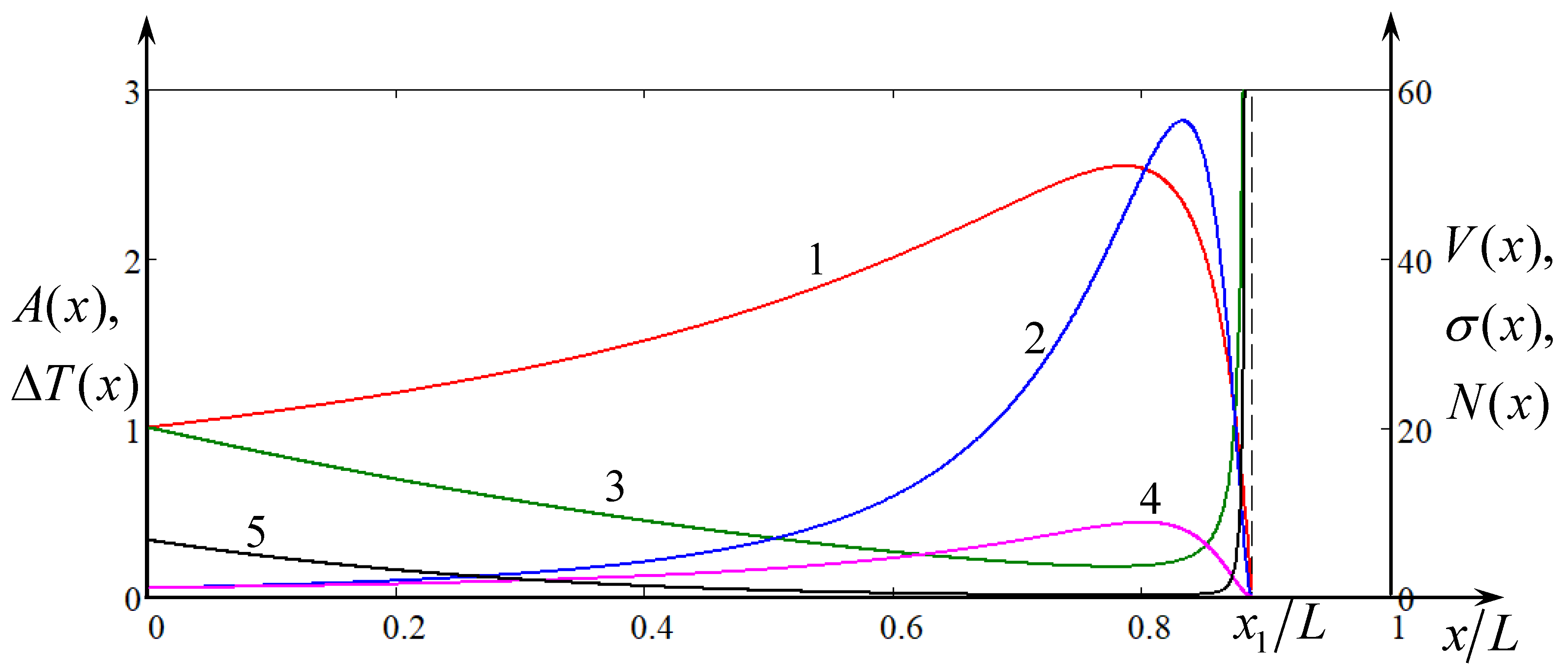
In the process of propagation towards the shoaling, a soliton experiences amplitude enhancement as per Equation (15) with simultaneous shrinking of its duration; its velocity V also increases with x in accordance with Equation (17). Variation of soliton amplitude, velocity, duration, as well as carrier wave period $T_c\left(x\right)=2\pi /\sigma \left(x\right)$ are shown in Figure 4. As one can see from this figure, both the amplitude and velocity increase first and attain the maximal values, but at different distances, after that they quickly decrease when the soliton approaches the distance where the lower and upper layers have equal thicknesses, and the nonlinear coefficient becomes zero (see lines 1 and 2 in Figure 4). In particular, the maximal soliton amplitude becomes 2.55 times greater than the initial one, whereas the maximal velocity becomes 57 times greater than the initial one. Note that a very similar effect of soliton amplitude decrease (while the duration increases) upon approaching the critical depth where $k{h}_c=1.363$ was revealed in Reference [25] when a soliton propagates in a non-rotating fluid with a smoothly varying bottom. In both cases (in this paper and in Reference [25]), the reason of soliton amplitude decrease is the vanishing of the nonlinear coefficients in the NLS equations, even though they vanish at different values of $kh$.

When x becomes greater than $x_1$, the soliton amplitude and velocity formally increase again and go to infinity when $x\to x_2$ (this is not shown in the plot). However, the adiabatic theory breaks much earlier, when $x\to x_1$, and the process of wave transformation in the vicinity of this point should be reconsidered more thoroughly, apparently, on the basis of primitive equations.

The soliton duration varies in an inversely proportional manner to the amplitude, therefore it decreases first, but then dramatically increases when $x\to x_1$ (see line 3 in Figure 4). In contrast to that, the period of the carrier wave increases first, attains a maximal value and then quickly drops to zero, when $x\to x_1$ (see line 4 in Figure 4). In the result of this, the number of carrier wave periods within the soliton half-duration $N\left(x\right)$ decreases first to zero and then formally increases again when $x\to x_1$ (see line 5 in Figure 4).

The transformation of soliton shape in the process of its propagation towards the coast is illustrated by Figure 3. The soliton shape half-way to the coast when $x=0.5L$ is still close to that of the NLS envelope soliton (see Frame (b)). However, at $x=0.7L$, where the soliton amplitude becomes close to the maximal value, it looks rather like a solitary wave, but represents a non-stationary formation oscillating in time (see Frame (c)). Such a formation can hardly be described by the TNLS equation which presumes that $N\left(x\right)>>1$.

Thus, in the process of soliton propagation towards the shoaling, it becomes narrower and transforms from the wave train shown in Frame (a) of Figure 3 to the pulse-type non-stationary solitary wave (a breather) as shown in Frame (c). To a certain extent, this behaviour is opposite to the transformation of the KdV solitary wave into the envelope soliton described, for example, in References [19,20,21,22].

7. Discussion and Conclusions

In the paper, it has been demonstrated that in a rotating fluid the most probable frequency of carrier wave which constitute the NLS solitary wave is the frequency where the growth rate of modulation instability is maximal. This agrees with the conjecture of Reference [24] and the numerical results of that paper. This frequency differs from the frequency where the group velocity has a maximum as was originally hypothesised in References [19,20,21]. An envelope solitary wave of this frequency can be described by the conventional TNLS Equation (7), rather than the generalised NLS Equation (18). Soliton solutions to both these equations have been presented and the limiting cases when some coefficients vanish have been discussed.

If an internal envelope soliton has been formed in a homogeneous two-layer rotating ocean and then enters a coastal zone, where the bottom linearly increases with a small gradient, then it experiences an adiabatic transformation. This leads to an increase in the soliton amplitude, velocity, and period of the carrier wave, whereas its duration decreases. Therefore, it becomes taller and narrower. At some distance it looks like a breather, i.e., a narrow non-stationary solitary wave. Apparently, the TNLS equation is not quite appropriate for the description of its further evolution; a more advanced theory and/or numerical simulation is required to this end. This can be a theme for further study.

References

- Grimshaw, R. Evolution equations for weakly nonlinear, long internal waves in a rotating fluid. Stud. Appl. Math. 1985, 73, 1–33. [Google Scholar] [CrossRef]
- Grimshaw, R. (Ed.) Internal solitary waves. In Environmental Stratified Flows; Kluwer Acad. Publ.: Dordrecht, The Netherlands, 2002; Chapter 1; pp. 1–27. [Google Scholar]
- Grimshaw, R.H.J.; Ostrovsky, L.A.; Shrira, V.I.; Stepanyants, Y.A. Long nonlinear surface and internal gravity waves in a rotating ocean. Surv. Geophys. 1998, 19, 289–338. [Google Scholar] [CrossRef]
- Grimshaw, R.; Guo, C.; Helfrich, K.; Vlasenko, V. Combined effect of rotation and topography on shoaling oceanic internal solitary waves. J. Phys. Oceanogr. 2014, 44, 1116–1132. [Google Scholar] [CrossRef]
- Helfrich, K.R.; Melville, W.K. Long nonlinear internal waves. Annu. Rev. Fluid Mech. 2006, 38, 395–425. [Google Scholar] [CrossRef]
- Ostrovsky, L. Nonlinear internal waves in a rotating ocean. Oceanology 1978, 18, 119–125. [Google Scholar]
- Ostrovsky, L.A.; Pelinovsky, E.N.; Shrira, V.I.; Stepanyants, Y.A. Beyond the KdV: Post-explosion development. Chaos 2015, 25, 097620. [Google Scholar] [CrossRef] [PubMed] [Green Version]
- Stepanyants, Y.A. The effects of interplay between rotation and shoaling for a solitary wave on variable topography. Stud. Appl. Math. 2019, 1–22. [Google Scholar] [CrossRef]
- Boegman, L.; Imberger, J.; Ivey, G.; Antenucci, J. High-frequency internal waves in large stratified lakes. Limnol. Oceanogr. 2003, 48, 895–919. [Google Scholar] [CrossRef] [Green Version]
- De la Fuente, A.; Shimizu, K.; Nino, Y.; Imberger, J. Nonlinear and weakly nonhydrostatic inviscid evolution of internal gravitational basin-scale waves in a large, deep lake: Lake Constance. J. Geophys. Res. 2010, 115, C12045. [Google Scholar] [CrossRef]
- Preusse, M.; Freistuhler, H.; Peeters, F. Seasonal variation of solitary wave properties in Lake Constance. J. Geophys. Res. 2012, 117, C04026. [Google Scholar] [CrossRef]
- Rojas, P.; Ulloa, H.N.; Nino, Y. Evolution and decay of gravity wavefield in weak-rotating environments: A laboratory study. Environ. Fluid Mech. 2018, 18, 1509–1531. [Google Scholar] [CrossRef]
- Ulloa, H.; Winters, K.; De la Fuente, A.; Nino, Y. Degeneration of internal Kelvin waves in a continuous two-layer stratification. J. Fluid Mech. 2015, 777, 68–96. [Google Scholar] [CrossRef]
- Galkin, V.M.; Stepanyants, Y.A. On the existence of stationary solitary waves in a rotating fluid. J. Appl. Maths. Mech. 1991, 55, 939–943. [Google Scholar] [CrossRef]
- Leonov, A.I. The effect of the Earth’s rotation on the propagation of weak nonlinear surface and internal long oceanic waves. Ann. N. Y. Acad. Sci. 1981, 373, 150–159. [Google Scholar] [CrossRef]
- Gilman, O.A.; Grimshaw, R.; Stepanyants, Y.A. Approximate analytical and numerical solutions of the stationary Ostrovsky equation. Stud. Appl. Math. 1995, 95, 115–126. [Google Scholar] [CrossRef]
- Ostrovsky, L.A.; Stepanyants, Y.A. Interaction of solitons with long waves in a rotating fluid. Physica D 2016, 333, 266–275. [Google Scholar] [CrossRef]
- Grimshaw, R.H.J.; He, J.-M.; Ostrovsky, L.A. Terminal damping of a solitary wave due to radiation in rotational systems. Stud. Appl. Math. 1998, 101, 197–210. [Google Scholar] [CrossRef]
- Grimshaw, R.; Helfrich, K.R. Long-time solutions of the Ostrovsky equation. Stud. Appl. Math. 2008, 121, 71–88. [Google Scholar] [CrossRef]
- Grimshaw, R.; Helfrich, K.R. The effect of rotation on internal solitary waves. IMA J. Appl. Math. 2012, 77, 326–339. [Google Scholar] [CrossRef]
- Grimshaw, R.H.J.; Helfrich, K.R.; Johnson, E.R. Experimental study of the effect of rotation on nonlinear internal waves. Phys. Fluids 2013, 25, 056602. [Google Scholar] [CrossRef] [Green Version]
- Grimshaw, R.; Stepanyants, Y.; Alias, A. Formation of wave packets in the Ostrovsky equation for both normal and anomalous dispersion. Proc. R. Soc. A 2016, 472, 20150416. [Google Scholar] [CrossRef] [PubMed] [Green Version]
- Whitfield, A.J.; Johnson, E.R. Rotation-induced nonlinear wavepackets in internal waves. Phys. Fluids 2014, 26, 056606. [Google Scholar] [CrossRef] [Green Version]
- Whitfield, A.J.; Johnson, E.R. Wave-packet formation at the zero-dispersion point in the Gardner—Ostrovsky equation. Phys. Rev. E 2015, 91, 051201(R). [Google Scholar] [CrossRef]
- Benilov, E.S.; Flanagan, J.D.; Howlin, C.P. Evolution of packets of surface gravity waves over smooth topography. J. Fluid Mech. 2005, 533, 171–181. [Google Scholar] [CrossRef]
- Benilov, E.S.; Howlin, C.P. Evolution of packets of surface gravity waves over strong smooth topography. Stud. Appl. Math. 2006, 116, 289–301. [Google Scholar] [CrossRef]
- Djordjevic, V.D.; Redekopp, L.G. The fission and disintegration of internal solitary waves moving over 2-dimensional topography. J. Phys. Oceanogr. 1978, 8, 1016–1024. [Google Scholar] [CrossRef]
- Andronov, A.A.; Fabrikant, A.L. Landau damping, wind waves and whistle. In Nonlinear Waves; Proc. Gorky School on Nonlinear Oscillations and Waves, Ed.; A.V. Gaponov-Grekhov: Moscow, Rusia, 1979; pp. 68–104. (In Russian) [Google Scholar]
- Churilov, S.M. Envelope solitons in an inhomogeneous medium. Fizika Plazmy 1982, 8, 793–796. (In Russian) [Google Scholar]
- Stepanyants, Y.A.; Fabrikant, A.L. Propagation of Waves in Shear Flows; Fizmatlit: Moscow, Rusia, 1992. (In Russian); Fabrikant, A.L.; Stepanyants, Y.A. World Scientific: Singapore, 1998. (In English) [Google Scholar]
- Karpman, V.I. Soliton evolution in the presence of perturbation. Phys. Scripta 1979, 20, 462–469. [Google Scholar] [CrossRef]
- Karpman, V.I. Nonlinear Waves in Dispersive Media; Nauka: Moscow, Rusia, 1973. (In Russian) [Google Scholar]
- Ostrovsky, L.A.; Potapov, A.I. Modulated Waves: Theory and Applications; World Scientific: Singapore, 1998. [Google Scholar]
- Zakharov, V.E.; Ostrovsky, L.A. Modulation instability: The beginning. Physica D 2009, 238, 540–548. [Google Scholar] [CrossRef]
- Apel, J.; Ostrovsky, L.A.; Stepanyants, Y.A.; Lynch, J.F. Internal solitons in the ocean and their effect on underwater sound. J. Acoust. Soc. Am. 2007, 121, 695–722. [Google Scholar] [CrossRef]
- Stanton, T.P.; Ostrovsky, L.A. Observations of highly nonlinear internal solitons over the continental shelf. Geophys. Res. Lett. 1998, 25, 2695–2698. [Google Scholar] [CrossRef] [Green Version]
Figure 1.
(Color online) Frame (a): line 1—free surface in the basin of the total depth m; line 2—position of a pycnocline at the depth m; line 3—normalised bottom profile as a function of . Frame (b): Normalised coefficients of the time-like Ostrovsky Equation (3): line 1—; line 2—; line 3—; line 4—; line 5—vertical line showing the distance where the upper and lower layers become equal; line 6—vertical line showing the distance where the thickness of the lower layer vanishes. Frame (c): Normalised coefficients of the TNLS Equation (7): line 1—; line 2—; line 3—; line 4—; line 7—.
Figure 2.
(Color online) A fragment of Frame (c) in Figure 1. Normalised coefficients of NLS Equation (7): line 4—; line 7—; line 8—; lines 5 and 6 are the same as in Figure 1.
Figure 3.
(Color online) An NLS envelope soliton of Equation (10) at (frame (a)), (frame (b)), and (frame (c)).
Figure 4.
(Color online) Variations with the distance of normalised soliton amplitude (line 1), velocity (line 2), duration (line 3), carrier wave period (line 4), and the number of carrier wave periods on the half-duration (line 5) when a soliton moves towards the shore with the linearly decreasing depth, as shown in Figure 1.
© 2019 by the author. Licensee MDPI, Basel, Switzerland. This article is an open access article distributed under the terms and conditions of the Creative Commons Attribution (CC BY) license (http://creativecommons.org/licenses/by/4.0/).
Share and Cite
MDPI and ACS Style
Stepanyants, Y.A. Dynamics of Internal Envelope Solitons in a Rotating Fluid of a Variable Depth. Fluids 2019, 4, 56. https://doi.org/10.3390/fluids4010056
AMA Style
Stepanyants YA. Dynamics of Internal Envelope Solitons in a Rotating Fluid of a Variable Depth. Fluids. 2019; 4(1):56. https://doi.org/10.3390/fluids4010056
Chicago/Turabian StyleStepanyants, Yury A. 2019. "Dynamics of Internal Envelope Solitons in a Rotating Fluid of a Variable Depth" Fluids 4, no. 1: 56. https://doi.org/10.3390/fluids4010056