Implementation and Validation of a Free Open Source 1D Water Hammer Code
by

Rune Kjerrumgaard Jensen
1,†, 
Jesper Kær Larsen
1,
Kasper Lindgren Lassen
1,
Matthias Mandø
2 and
Anders Andreasen
3,* 1
Aalborg University Esbjerg, Niels Bohrs Vej 8, 6700 Esbjerg, Denmark
2
Department of Energy Technology, Aalborg University Esbjerg, Niels Bohrs Vej 8, 6700 Esbjerg, Denmark
3
Studies & FEED, Field Development, Rambøll Energy, Bavnehøjvej 5, 6700 Esbjerg, Denmark
*
Author to whom correspondence should be addressed.
†
Current address: Process Department, Field Development, Rambøll Energy, Bavnehøjvej 5, 6700 Esbjerg, Denmark.
Fluids 2018, 3(3), 64; https://doi.org/10.3390/fluids3030064
Submission received: 9 August 2018
/
Revised: 24 August 2018
/
Accepted: 29 August 2018
/
Published: 3 September 2018
Abstract
:This paper presents a free code for calculating 1D hydraulic transients in liquid-filled piping. The transient of focus is the Water Hammer phenomenon which may arise due to e.g., sudden valve closure, pump start/stop etc. The method of solution of the system of partial differential equations given by the continuity and momentum balance is the Method of Characteristics (MOC). Various friction models ranging from steady-state and quasi steady-state to unsteady friction models including Convolution Based models (CB) as well as an Instantaneous Acceleration Based (IAB) model are implemented. Furthermore, two different models for modelling cavitation/column separation are implemented. Column separation may occur during low pressure pulses if the pressure decreases below the vapour pressure of the fluid. The code implementing the various models are compared to experiments from the literature. All experiments consist of an upstream reservoir, a straight pipe and a downstream valve.
1. Introduction
Sudden changes to fluid flow in piping may result in the generation of a pressure surge or a chock wave travelling at the speed of sound. The flow changes may be induced by e.g., pump starting/stopping, pipe rupture/leakage, valve opening/closing etc. The phenomenon is referred to as Water Hammer and is most common for liquid flow, due to the low compressibility of water. Probably the most common water hammer is when a downstream valve closes suddenly. When the valve closes, the liquid column upstream is still moving and when the liquid column is slowed down, the kinetic energy is converted to pressure head. The pressure pulse created is noisy and the pressure pulse may have a magnitude which causes pipe rupture or resulting in other equipment damage. Water hammer may be observed in a variety of applications e.g., in power plant steam generation/cooling systems [1,2], district heating system [3], hydro-power [4], irrigation systems [5,6], domestic plumbing [7], pipeline transport of oil and chemicals [8,9] etc. It is important to be able to accurately model the physical phenomenon for correct dimensioning of pipes, adequate choice of valve closing time etc. to prevent damages.
The water hammer phenomenon is fully described by the continuity and momentum equations. Different methods for solving these equations exist, e.g., the Finite Volume Method (FVM) [10], the Finite Difference Method (FDM) [11,12], the Finite Element Method (FEM) [13], and the Method of Characteristics (MOC) [14]. The most popular method is the explicit MOC because it is relatively easy to implement and it has a relatively high accuracy [15].
In this paper an implementation of the MOC proposed by [15] will be demonstrated. The MOC is discretized and implemented in Octave [16]/MATLAB® (The MathWorks, Natick, MA, USA). A number of different friction models are implemented, as well as two different methods for handling column separation/cavitation. As a part of the present paper, the full source code is provided, in order for anyone to explore the code and freely use it for their own studies and for further improvement. Many commercial tools are available in the market, a vast amount already summarised by [14]. The authors find it important to have a tool which is easy to modify and extend in order to e.g., explore different solution schemes, grid types, friction models etc. Furthermore such code may find potential usage in applications such as failure analysis [17], condition monitoring [18], and aid the design of protective measures in order to avoid e.g., pipeline rupture [19]. By sharing the source code, the authors hope, at least partially, to contribute to achieving this goal. The full verbatim code is provided in the Appendix A of the present paper and further it is available for download [20]. In the present paper the code and the implementation of the different friction and cavitation models are validated against experimental data from the literature. The different implemented models will be investigated and quantitatively compared.
2. Theory and Model Implementation
2.1. Water Hammer Equations and Method of Characteristics
The water hammer phenomenon is described by the continuity equation in Equation (1) and the momentum equation in Equation (2) [21,22].
where g is the gravitational acceleration, H is the piezometric head, t is time, A is the cross-sectional area of the pipe, Q is the volumetric flow rate, x is position in the axial direction, J is the friction term, and is the angle from horizontal. In the equations, it is assumed that the cross sectional area and the wave speed, a, are constant, and that which means that the convective terms can be neglected. It is also assumed that the flow is one dimensional and that the compressibility and flexibility of the pipe is accounted for in the wave speed as seen in Equation (3).
where is the density of the fluid, K is the bulk modulus of the fluid, E is Young’s modulus of the pipe, D is the inner pipe diameter, e is the pipe wall thickness, and is a coefficient describing the relation to Poisson’s ratio, .
The method used to solve the set of Partial Differential Equations (PDEs) is the MOC. The MOC transforms the set of PDEs into the four Ordinary Differential Equations (ODEs) seen in Equations (4) and (5).
The equations in Equation (4) can be solved along the characteristic lines with the slope determined by Equation (5), as is illustrated in Figure 1. By use of the characteristic lines, point P can be found using point A and B. This is done by the positive characteristic line, , corresponding to a positive a and the negative characteristic line, , corresponding to a negative a. In this case the characteristic lines are linear, since it is assumed that a is constant.
Approximating Equation (4) with finite differences and integrating along the positive characteristic line and along the negative characteristic line yield Equations (6) and (7), where and are described with Equations (8) and (9), respectively and .
Inserting Equation (6) into Equation (7) and solving for yields:
can then be calculated with Equation (11).
Equations (6) to (9) are used in a rectangular grid to simulate the water hammer. The friction term J is evaluated explicitly.
A rectangular grid is chosen over the less computationally intensive diamond grid to enhance the plotting of the pressure distribution. Note that the rectangular grid, which consists of two independent diamond grids, tends to generate small unphysical oscillations, which are visible on the plots.
2.2. Steady State
In the previous section the values at point A and B are assumed to be known which means that the steady state of the system has to be determined. In steady state the volumetric flow rate is constant through the pipe. The head through the pipe is calculated with Equation (12).
2.3. Friction
The estimation of the water hammer pressure propagation is largely dependent on the friction forces. Traditionally, the friction is modelled as steady or quasi-steady. The steady and quasi-steady friction is able to predict the pressure at the first pressure peak, but as the wave propagates, the dampening of the pressure is not sufficient [23]. For engineering design, the first and thereby largest pressure peak, for single phase flows, is of primary interest. However, there are also specific situations where the secondary pressure peaks are of interest [24]. An example of this is in the cooling system of a nuclear power plant, where a quick restart of the cooling system is necessary. Another example can be quick restart of (off-shore) oil and gas production facilities in order to reduce loss of production etc. If there are sensitive components behind the closed valve, it is necessary to wait for the water hammer to dissipate to a sufficiently low pressure, at which the sensitive components can survive without damage [25].
A method to accurately describe the dampening of the pressure peak is by modelling the unsteady friction. It is complex and more computationally heavy to model unsteady friction compared to modelling steady friction, but unsteady friction modelling is essential for a more precise estimation of the transient behavior [24]. Unsteady friction models fall into three main groups.
- Convolution Based (CB)
- Instantaneous Acceleration Based (IAB)
- Extended Irreversible Thermodynamics (EIT)
The CB friction models are dependent on the convolution of the history of accelerations with a weighting function. This was first derived by Zielke [26] for laminar flow. Work has been carried out to extend Zielke’s CB model to the turbulent regime by Vardy and Brown, assuming a bilinear turbulent viscosity distribution for both smooth pipes [27] and fully rough pipes [28]. Zarzycki et al. [29] derived a more advanced CB friction model for turbulent flow assuming a four-region turbulent viscosity model.
The IAB model suggested by Brunone et al. [30] is dependent on the instantaneous acceleration, the convective acceleration, and a damping coefficient. The damping coefficient can be found either empirically as suggested by [30] or as will be used here, the theoretical values derived by Vardy and Brown [27,28]. The determination of the damping coefficient can be done from the initial Reynolds number as a constant or updated on the local Reynolds number, which has been shown to give better results [31]. IAB models with two damping coefficients exist [32,33], but they are not covered herein because there is no analytical way of determining these and therefore they have to be determined empirically.
The EIT derived by Axworthy et al. [34] is a physically well described model, but it has a relaxation time that is usually determined empirically. Storli and Nielsen [35] have derived values based on position dependent coefficients from CB models.
The friction term J consists of a quasi-steady friction term and an unsteady friction term as in Equation (13) [22].
The quasi-steady friction term is the skin friction of the pipe and it is modelled using Equation (14).
where is the quasi-steady Darcy friction factor which is updated for the local flow.
The unsteady friction is modelled with both convolution based friction models, and an instantaneous acceleration based friction model.
2.4. Convolution Based Friction Models
The convolution based friction model was developed by Zielke [26] for laminar flow. The unsteady friction is dependent on the convolution of past accelerations with a weighting function as seen in Equation (15).
where is the dynamic viscosity of the fluid and is the weighting function, which is dependent on the dimensionless time , defined as in Equation (16).
All the CB models are defined as in Equation (15) with different weighting functions. The CB models are implemented in a rectangular grid with first order finite difference approximations as in Equation (17) [36].
where i is the spatial index, j is the time index, and is the number of time steps from the beginning of the closure of the valve. It should also been noted that in the implementation of the accelerations in the code, the acceleration vector is filled from the bottom of the vector for simplifying the convolution with the weighting function. Equation (17) is evaluated at both the positive and negative characteristics.
The weighting function suggested by Zielke is defined as in Equation (18).
where 0.282095, −1.25, 1.057855, 0.9375, 0.396696, −0.351563} and 26.3744, 70.8493, 135.0198, 218.9216, 322.5544}.
Vardy and Brown [27,28] extended the range of applicability to the turbulent flow regime for Reynolds numbers up to with a two-region turbulent viscosity model. In the two-region turbulent viscosity model, it is assumed that the turbulent viscosity varies linearly from the wall to the core region and is constant in the core region. It is also assumed that the viscosity distribution is constant over time. The approximated weighting function derived for a smooth pipe has the form as seen in Equation (19) [27].
where , , , and it is assumed that the eddy viscosity at the wall is equal to the laminar viscosity, i.e., .
2.5. Instantaneous Acceleration Based Friction Models
In the instantaneous acceleration based friction model, suggested by Brunone et al. [30], the unsteady friction is dependent on the instantaneous acceleration, the instantaneous convective acceleration and a damping coefficient as in Equation (21), with the sign correction suggested by Vítkovský [37].
where k is Brunone’s friction coefficient, which describes the damping of the head, is the local instantaneous acceleration, and is the instantaneous convective acceleration. The implementation of the IAB model has been done explicitly with first order finite differences as in Equation (22) for the positive characteristic and as in Equation (23) for the negative characteristics.
Brunone’s friction coefficient, k, can either be determined empirically [30] or analytically via Vardy’s shear decay coefficient, , as in Equation (24) [37].
Vardy’s shear decay coefficient for laminar flow is defined as in Equation (25) and for turbulent flow, in smooth pipes, as in Equation (26) [37].
The analytical solution is based on the CB model suggested by Vardy & Brown, where Vardy’s shear coefficient is derived as a limiting value of the unsteady friction coefficient with the special case of constant acceleration.
2.6. Boundary Conditions
All the experiments were conducted with a single pipe with a reservoir at the upstream boundary and a valve at the downstream boundary. Therefore, it was necessary to implement the reservoir and valve boundary conditions in the code.
2.6.1. Reservoir
When using a reservoir, it is assumed that the reservoir is large enough, so that elevation changes during operation can be neglected. The head at the reservoir is assumed to be constant, , and the flow rate can be isolated from Equation (7).
2.6.2. Valve
When applying a valve, it is important to correctly describe the closure, since it affects both the magnitude and the shape of the pressure peak. It is possible to approximate the valve behaviour using Equation (27) [21].
where is the dimensionless valve closure time, is the actual closure time, t is the time, and m is an adjustable constant. If m is set to zero, then the valve is assumed to close instantaneously which yields the maximum pressure peak. The behaviour of is illustrated in Figure 2 for . When , there will be a rapid decrease in flow rate at the beginning and a slow decrease at the end of the closure. For there will be a linear fall in flow rate during the closure. When , there will a slow decrease in flow rate at the beginning and a rapid decrease at the end of the closure. The flow rate can be calculated with Equation (28).
where and 0 denotes steady state values.
2.7. Column Separation and Cavitation
If the pressure during a low pressure period for a liquid-filled pipe reaches the vapour pressure, the water starts to evaporate. This evaporation will form vapour bubbles and cavities. A subsequent increase in pressure will cause the bubbles to collapse. This phenomenon often referred to as cavitation or column separation has been implemented in the code by two different models–the Discrete Vapour Cavity Model (DVCM) [15,21] and the Discrete Gas Cavity Model (DGCM) [38].
Both the DVCM and the DGCM models assume that the wave speed is not affected by the amount of free gas. It is also assumed that all the free gas in each reach is present in a single pocket at the node causing the wave speed to be constant and identical to the wave speed for a single phase system between each node. The gas pocket at the node is modelled with Equation (29) [21].
where is the volumetric flow rate exiting the node and is the volumetric flow rate entering the node. To determine the volume of the gas pocket, Equation (29) can be integrated from time to time t, and the result is given in Equation (30) [21].
where is the volume of the gas pocket, Q is the volumetric flow rate, the subscript P indicate points at time t, indicate points at time , u indicate volumetric flow rate entering the node, and is a weighting factor.
The volumetric flow rates are illustrated in Figure 3. It can be seen that there is a modification to the negative characteristics equation, , since it goes from and not . Therefore the in Equation (9) is replaced with and is calculated by Equation (31).
The weighting factor controls the weight of the values at t and at . With only values at are used and with only values at t are used. It is generally recommended to keep above as an over reliance of old values have shown to give excessive numerical oscillation. A value close to is expected to give the most accurate results, but at this low value some numerical oscillations may still be present. The numerical oscillation is primarily present when gas cavity sizes are small, i.e., in the high pressure zones of the water hammer event. To decrease the numerical oscillations, the value of can be increased towards unity. However, this will cause more spreading of rarefaction waves which can result in increased attenuation. Setting will remove all numerical oscillations, but will introduce the largest amount of attenuation. Therefore it is recommended to choose a value of as close to as possible while experiencing minimal oscillation [21].
2.7.1. Discrete Vapour Cavity Model
DVCM is the simplest of the two phase models included in the program, and it can be used for many flow conditions [21]. However, as will be seen later, DVCM has its limitations when the void fraction becomes too high. Therefore it is recommended to only use DVCM when the void fraction is below 10% [39].
It is assumed that there is no free gas in the system, and that at steady state, and when the pressure is above the vaporization pressure, there is no vapour present in the system, . The flow can therefore be treated as a single phase system, where the volumetric flow rates can be set equal to each other, , because the difference between them describes the increase in vapour volume for each time step. When the pressure becomes lower than or equal to the vaporization pressure, the nodes are treated as boundary nodes, with a fixed pressure as described in Equation (32) [21].
When the head in the node is known, it is possible to calculate the volumetric flow rates and the vapour cavity size with Equation (11), (30) and (31) respectively, where and are replaced with and .
DVCM—Steady State
As described earlier, DVCM assumes that flow at steady state can be treated as a single phase system, with , and it is therefore calculated as described in Section 2.2.
DVCM—Boundary Conditions
The upstream reservoir is calculated as in Section 2.6.1, with , because it is assumed that the pressure in the reservoir is always above the vaporization pressure.
For the downstream valve, the outlet volumetric flow rate, , is described as in Section 2.6.2, while the nodes are treated in a similar fashion as in Section 2.7.1. The difference between the calculation method for the interior nodes, see Figure A2 in Appendix A.1, and the valve boundary, is that Equation (10) is replaced with and Equation (33) in the flowchart, while Equation (11) is replaced with Equation (28) in the flowchart in Appendix A.1.
2.7.2. Discrete Gas Cavity Model
DGCM is the more complex model, of the two phase models included in the program, and it can be used for many flow conditions.
In DGCM, it is assumed that there is always a small amount of free gas present in the system, and because there is always a small amount of free gas present, it is not possible to calculate the flow as in DVCM. A new expression for the head, which takes into account the effect of the gas cavity, has to be implemented. This is done via Equation (30), where Equation (31) is used to describe and Equation (28) is used to describe . This results in Equation (30) with two unknown parameters, and . can be described with the ideal gas law, as seen in Equation (34), where it is assumed that the mass of free gas, , is constant.
is the gas constant, T is the temperature, is the absolute partial pressure of the free gas, and is the absolute partial pressure for the initial void fraction (i.e., at steady state). is isolated from Equation (34) and a simplified form can be seen in Equation (35), where is described with Equation (36).
is a constant which is calculated with Equation (37).
With the expression for in Equation (35), Equation (30) will have the form seen in Equation (38), remembering that and are described with Equations (31) and (28) respectively.
Equation (38) can be rearranged into Equation (39).
where , , , and are defined as in Equation (40).
Equation (39) can be solved as a quadratic equation, where x is the variable. The result can be seen in Equation (41), where the two first expressions are isolated from the roots of the quadratic equation. The third and fourth expressions are linearised versions of the two first expressions, which can produce inaccurate results in extreme conditions of high pressure and very low void fraction, or at very low pressure and high void fraction, where . The fifth expression is for the case when .
With the head described as in Equation (41), the volumetric flow rates and the gas cavity size are calculated with Equations (31), (11), and (30) respectively.
DGCM—Steady State
For the steady state conditions, DGCM uses the same calculation method as for single phase flow, Section 2.2, with the addition of the calculation of the gas cavity size. At steady state Equation (34) can be simplified to Equation (42) because .
DGCM—Boundary Conditions
For DGCM, the upstream reservoir uses the same calculation method as for single phase flow, Section 2.6.1, with the addition of the calculation of the gas cavity size. The gas cavity size is calculated with Equation (35), where is replaced with .
For the downstream valve, the same method for calculating the outlet volumetric flow rate, , as in Section 2.6.2 is used. The expression for the head is derived in a similar fashion as to Section 2.7.2, but this time an expression for is not needed in Equation (30), as it is now described with Equation (28). This gives the expression in Equation (43), which can be rearranged in Equation (44).
where , , , and are defined as in Equation (45).
3. Experimental
Previous articles have compared CB and IAB friction models to a single experiment, where a friction model is recommended for a single experiment [40,41]. In this article, three CB friction models and one IAB friction model will be compared to three different experiments to establish how the different friction models behave under different experimental conditions. As for the implementation of different friction models, the implemented cavitation models are compared to experiments from the literature.
The experiments chosen consist of a single pipe between a reservoir/pressure tank at the upstream end and a fast closing valve at the downstream end as seen in Figure 4.
The different friction models are compared with experimental results found in literature. The pressure is evaluated at the valve position. The selected experiments vary in pipe material, diameter, length, thickness as well as flow velocity in an attempt to see how these differences affect, prediction of the water hammer phenomenon. An overview of the different parameters is found in Table 1.
It is attempted to cover a wide variety of flow conditions to test the implemented models. The three chosen experiments for validating the different implemeted friction models have a Reynolds number of 52052, 15843, and 8453, respectively. The experiments used for comparing the different cavitation models have Reynolds number of 6605, 9894 and 30823, respectively.
3.1. Experiment 1
The experimental study conducted by Traudt et al. [42] consist of a m stainless steel pipe (grade ) with a diameter of 19 mm and a wall thickness of mm. Young’s modulus is set to 200 GPa, the pipe roughness to m, and Poisson’s ratio to . The test section has a high-pressure tank at the upstream end and a fast acting valve, with a closure time of 18 ms, at the downstream end. The piping also has a upwards slope. The initial flow velocity is m/s with a head at the reservoir of 433 m. For the simulation, m is set to , which was the best fit for the valve closure, as is not reported by Traudt et al. The fluid in the study is water at room temperature.
3.2. Experiment 2
The experimental study conducted by Adamkowski and Lewandowski [40] consists of a 98 m copper pipe in a spiral coil with an inner pipe diameter of 16 mm and a wall thickness of mm. Young’s modulus and Poisson’s ratio are reported in the article at 120 GPa and GPa, respectively. The roughness was not stated by [40]. For the present investigation, a roughness of m is used corresponding to a typical value of copper. The test section has a high-pressure tank at the upstream end and a quick-closing spring driven ball valve, with a closure time of 3 ms, at the downstream end. The test section has a reported maximum inclination angle of less than . Because of the uncertainty of the inclination and its small size it is neglected in the simulations. The initial flow velocity is m/s with a head at the reservoir of 128 m. For the simulation, m is chosen as , which was the best fit for the valve closure as is not reported by Adamkowski et al. The fluid in the study is water where the density, viscosity, and bulk modulus was given at 1000 kg/m, kg/m· s, and GPa, respectively.
3.3. Experiment 3 and 4
The experimental study conducted by Soares et al. [41] consists of a m straight copper pipe with an inner diameter of 20 mm and a wall thickness of mm. The test section has a hydropneumatic tank at the upstream end and a pneumatically actuated quarter turn ball valve at the downstream end. The closure time for the valve is not described and therefore it is approximated by the time it takes to reach maximum pressure from steady state pressure. The closure time is estimated at 18 ms. Two experiments were conducted by Soares et al. with an initial velocity of m/s (Experiment 3) and m/s (Experiment 4). The lowest velocity resulted in a single phase water hammer, whereas the largest velocity resulted in a two phase water hammer. The head at the reservoir is 46 m for the two experiments. For the simulation, m is chosen as 3, which was the best fit for the valve closure as were not described by Soares et al. The material properties for the copper pipes were not given in the study, and the properties from experiment 2 were used. The fluid used in the study is water and the experiment is conducted at C.
3.4. Experiment 5 and 6
The experimental study conducted by Bergant et al. [43] consists of a m straight copper pipe with an inner diameter of mm and a wall thickness of mm. The test section has a pressurized tank at the upstream and the downstream end of the pipe. To generate the transient, a fast closing valve is placed at the downstream end of the pipe. The pipe has an inclination of . Two experiments have been conducted with an initial velocity of m/s (experiment 5) and m/s (experiment 6) which resulted in column separation. The closure time for both experiments in s and the head at the upstream pressurized tank is 22 m. The material parameters were not given by [43], therefore the same parameters used for the [41] experiments is used for experiment 5 and 6 as the pipes consists of the same material. For the simulation, m is set to 5, which was the best fit for the valve closure, as is not reported by [43]. Water is the working fluid at room temperature.
4. Results and Discussion
In this section the results for the single phase simulations of experiments 1, 2 and 3 and the column separation simulations of experiment 4, 5 and 6 will be presented and discussed. In addition to this, the code has been benchmarked against computational fluid dynamics (CFD) simulations. The results are presented elsewhere [44]. Good agreement was found both for with and without column separation when unsteady friction modelling was applied in the MOC code.
4.1. Single Phase
A grid independence study showed no difference for the steady and quasi-steady friction models. For the unsteady friction models the head varied from 12 to 24 reaches, but hereafter the change was insignificant. Therefore all single phase simulations are performed with 24 reaches.
Figure 5 and Table 2 show the results of the different friction models for experiment 1. The mean oscillation frequency of the experiment is found at Hz which is lower than the frequencies calculated with the Steady and Quasi-Steady friction models with the fastest frequency of Hz, followed by Brunone with Hz and the CB friction models with a frequency of Hz. This causes a phase offset between the experimental and simulated data, which is evident in Figure 5 after the third high pressure peak. At the end of the data the phase offset is almost half an oscillation.
It can be seen that all the friction models have the same tendency at the first peak and are able to accurately estimate the head of the peak with only a slight overestimation. At the third pressure peak, the CB friction models accurately model the friction with an overestimation of the head in the range of 0.43–0.50%, whereas the other friction models start to underestimate the friction. At the tenth pressure peak, none of the friction models accurately describe the dampening of the head with the Steady and Quasi-Steady friction models overestimating the head with % and %, the Brunone friction model with % and the CB models with 10.33–10.52%. From Table 2, it can be seen that the CB based models gives the best prediction of the experimental results.
The experimental results [42] indicate some double peaks, which are not predicted by any of the friction models. This is believed to be caused by harmonics of the experimental setup. As such Traudt et al. [42] report that the second harmonic frequency of the experimental setup of 132 Hz is interfering with the frequency of the water hammer which is 43 Hz. Since none of the models accurately describe the experimental data, a sensitivity analysis on the parameters, Young’s modulus, Poisson’s ratio and the temperature of the water were conducted to see, whether this could explain the difference. Both Young’s modulus and Poisson’s ratio are varied % and the temperature of the water C. Decreasing the Young’s modulus and the temperature and increasing the Poisson’s ratio individually improved the results slightly compared to the experiment, but not enough to explain the difference. Investigating combined effects also showed an improvement compared to the experimental data, but again it could not explain the difference. Therefore, there must be an effect in the experiment that causes extra damping on the head and a slower oscillation frequency that is not taken into account in the friction models.
In Table 2, an average calculation time, for five identical simulations, for each friction model can be seen, together with a normalized calculation time, where the reference time is the average calculation time for the steady friction model. It can be seen that as the complexity of the friction model increases, so does the calculation time, where a significant increase is seen when going from Brunone’s unsteady friction model to the CB models. The reason for this increase is because of the convolution in the CB models, which uses all of the calculated volumetric flow rates in the used nodes, while Brunone only uses the volumetric flow rate from the two previous time steps.
The oscillation frequency for all the models is close to the experimental, see Table 3. Looking overall on the first peak, the steady, quasi-steady and Brunone coincide best with the data, and all three CB friction models seem to overestimate the head slightly, but it is close to the highest peak in the experimental data with a difference of % for Vardy and Brown, % for Zielke and % for Zarzycki. The head at the valve in steady state is lower for the experiment compared to the simulations, which could be because of an underestimation of the steady state friction. Initially, the friction models suggested by Zielke and Zarzycki render the most accurate representation of the dampening of the head and at the third pressure peak, only underestimating the head by % and %, respectively. This is followed by the friction model by Brunone with an overestimation of %, the Quasi-Steady model with %, the Steady model with %, and the model by Vardy and Brown with %. At the tenth pressure peak, the picture is different with the model by Vardy and Brown giving the most accurate representation with an overestimation of the head by % followed by the model by Brunone with an overestimation of %, the model by Zielke with an underestimation of %, the model by Zarzycki with an underestimation of %, the Quasi-Steady model with an overestimation of %, and the Steady model with an overestimation of %. The behaviour of the steady, quasi-steady and Brunone models is not reminiscent of the experimental results. The CB based models behaviour is reminiscent of the experimental data with the Vardy & Brown model being the closest to the experimental. The difference in the CB friction models is attributed to the difference in the weighting functions and their dependency on the Reynolds number. Overall, it is the model by Vardy & Brown that provides the best representation.
In Table 3, the average calculation time is summarised. It can be seen, that as the complexity of the friction model increases, the calculation time increases, which was also seen for experiment 1.
Figure 7 and Table 4 show the results of the different friction models for experiment 3. The oscillation frequency of the models, ranging from to Hz, is close to the experimental one, at Hz, therefore no offset between the experimental data and the simulations is expected, and it is also evident in Figure 7. The head at steady state is larger for the simulations than the experiment, which could be due to an underestimation of the steady state friction.
All the friction models slightly overestimate the first pressure peak with steady and quasi-steady giving the best estimation with an overestimation of % and %, respectively, Brunone being comparable with an overestimation of % and the CB friction models with an overestimation ranging from % to %. Part of the overestimation of the models is likely caused by the overestimation of the steady state head. The model by Brunone represents the dampening of the head most accurately by overestimating the head with % at the third pressure peak and with % at the tenth pressure peak, followed by the CB friction models overestimating the third pressure peak in the range 2.05–2.19% and for the tenth pressure peak 1.70–2.28%, the Steady and Quasi-Steady models overestimating the third peak with % and %, and for the tenth peak with % and %.
In Table 4, the average calculation time is summarised. The same trend as for experiment 1 and 2 is observed.
For all the experiments, it can be seen that the steady and quasi-steady friction models accurately estimate the first peak of the pressure wave, but do not accurately describe the damping of the pressure wave. There is almost no difference in the head of steady and quasi-steady, which means that there is little to no gain from calculating the friction factor for each node and time step which is done in the quasi-steady model. If a precise estimation of the wave propagation is wanted, an unsteady friction model shall be used. A general behaviour for the experiments with copper pipes (experiments 2 and 3) is that the friction in the pipe in steady state is underestimated. This can be due to some of the material properties chosen for the simulations not exactly matching the real properties.
Based on the four experiments, the Vardy & Brown friction model is recommended as a generic choice. The friction model has a good estimation of the wave behaviour and propagation. The head of the friction model is in neither of the experiments underestimated, as e.g., Zielke and Zarzycki in experiment 2.
4.2. Column Separation
For both DVCM and DGCM for all three experiments, a grid test was made and it showed that a grid of 24 to 48 reaches was sufficient. Compared to single phase model, an additional parameter (the weighing factor, ) had to be tuned for the two phase models. It is recommended that is set to and it was found that values close to this was adequate. It was also found that the best results were obtained for both column separation models in combination with the friction model suggested by Vardy & Brown. Further information of the grid test, choice of , and results obtained by the other friction models are found in [44].
The oscillation frequency of both DVCM and DGCM are close to the one obtained from the experimental data of Hz. In the first high pressure zone it can be seen that DVCM and DGCM give almost identical results both overestimating the pressure by %. In the second high pressure zone the large pressure peak is caused by the implosion of bubbles. Both models give an overestimation of the second high pressure peak with DVCM giving an error of %. In the third pressure zone neither of the models are able to model the largest pressure peak with DVCM underestimating the pressure peak by % and DGCM by %. However, both models have a maximum pressure exceeding this pressure in the previous pressure peak, and is therefore still conservative although slightly inaccurate. On the tenth peak DVCM gives the best results overestimating the head by % compared to DGCM by %. Overall the DVCM is the best model for experiment 4.
In Table 5, it can be seen that the calculation time for DVCM and DGCM is very similar, and hence the added complexity of DGCM does not extend the calculation time significantly. Figure 9 and Table 6 show the results obtained with DVCM and DGCM for experiment 5.
The oscillation frequency is larger for both DVCM, Hz, and DGCM, Hz, than the one obtained by the experimental data, Hz. Thus, the models are expected to oscillate faster than the experiment, which is also clear for DVCM. For DGCM it seems that there is almost no difference between the oscillation of the model and the experiment. This means that the oscillation of the pressure wave is accurate but that the timing of the pressure peaks are off.
In the first high pressure zone both models give similar results overestimating the pressure by % or %. For the second pressure peak both models give a good approximation of the pressure with DGCM giving the best approximation with an overestimation of %. In the third high pressure zone there is two high pressure peaks; one in the beginning and one in the end. Neither of the models are able to model the pressure peak in the beginning of the third pressure zone, but both are able to model the pressure peak in the end. This pressure peak is most accurately modelled by DGCM with an overestimation of % compared to an underestimation of % with DVCM. In the seventh pressure zone DVCM gives the best results with an overestimation of the pressure by % compared to % obtained with DGCM. Overall DGCM gives the best result as it accurately model the oscillation of the pressure wave and provides the best results when cavitation is occurring.
In Table 6, it can be seen that the calculation time for DVCM and DGCM is very similar, as was the case with experiment 5, and hence the complexity of DGCM does not extend the calculation time significantly.
In this experiment only the DGCM gives satisfactory results. The DVCM model has a way too fast oscillation and dampening of the pressure, giving unrealistic results. Therefore, the results obtained from DVCM have been omitted. This failure to obtain realistic results is attributed to the large void fractions obtained, which is known to cause problems for the DVCM.
Comparing the oscillation frequency of the DGCM with the experiment it is clear that they are almost identical at Hz and Hz respectively. Therefore almost no offset between the experimental data and the simulated data are expected, as is also evident in Figure 10. The DGCM give accurate results for the first three pressure zones never overestimating the pressure by more than %. However, at the fourth pressure zone the simulated data starts to exhibit some oscillations causing an overestimation of %.
In Table 7, the calculation time for DGCM is shown. The reason for the calculation time being lower than experiment 5, while still with a higher flow time, is due to experiment 5 using 48 reaches, while experiment six uses only 24 reaches.
The overall best model for cavitation/column separation is considered to be the DGCM. It is more robust and provides accurate results of the pressure while never underestimating the maximum pressure. DGCM is recommended as a generic choice.
5. Conclusions
In this paper an implementation of a code for simulation of pressure transients in liquid-filled piping both with and without cavitation/column separation has been presented. The solution scheme implemented for simulating water hammer is the MOC.
For single phase/ liquid-filled pipe water hammer, six friction models are implemented and tested against three different experiments found in literature. The friction models consist of a steady, quasi-steady, and four unsteady models. The unsteady friction models consist of three CB models (Zielke, Vardy and Brown, and Zarzycki) and one IAB model (Brunone). For the experiments included in the present study the Vardy and Brown model seems to provide the best results.
Two models for taking the effects of cavitation/column separation into account have been implemented, the DVCM and DGCM models. The two models are compared to three different experiments. For all experimental comparisons the Vardy and Brown CB friction model has been applied. For the included experiments the DGCM gives the best results overall, although the DVCM provides a slightly better fit for a single experiment.
Generally, it is found that employing unsteady friction models the presented code is adequately able to simulate the chosen experiments.
The authors provide the full verbatim source code to the presented MOC implementation along with the present paper. In doing so, the authors hope that the code can find good use for others.
Author Contributions
Conceptualization, A.A. and M.M.; Data curation, R.K.J., J.K.L. and K.L.L.; Methodology, R.K.J., J.K.L. and K.L.L.; Software, R.K.J., J.K.L. and K.L.L.; Validation, R.K.J., J.K.L., K.L.L., A.A. and M.M.; Formal Analysis, R.K.J., J.K.L. and K.L.L.; Investigation, R.K.J., J.K.L. and K.L.L.; Writing—Original Draft Preparation, R.K.J., J.K.L., K.L.L. and A.A.; Writing—Review and Editing, A.A. and M.M.; Supervision, A.A and M.M.
Funding
This research received no external funding.
Acknowledgments
Language secretary Susanne Tolstrup, Field Development, Ramboll Energy, has kindly provided her assistance for proofreading this manuscript.
Conflicts of Interest
The authors declare no conflict of interest.
Abbreviations
The following common symbols are used in this manuscript:
| Void fraction, − | |
| Difference, − | |
| Pipe roughness, m | |
| Dynamic viscosity, kg/m· s | |
| Kinematic viscosity, m/s | |
| Poisson’s ratio, − | |
| Density, kg/m | |
| Dimensionless time, − | |
| Dimensionless closing time, − | |
| Pipe inclination, | |
| Weighting factor, − | |
| ∗ | Convolution operator, − |
| A | Cross sectional area, m |
| a | Single phase wave speed, m/s |
| Two phase wave speed, m/s | |
| B | Pipe constant, s/m |
| Poisson’s ratio dependent constant, − | |
| Vardy shear decay coefficient, − | |
| D | Inner pipe diameter, m |
| E | Young’s modulus, Pa |
| e | Thickness of the pipe wall, m |
| f | Darcy’s friction factor, − |
| g | Gravitational acceleration, 9.81 m/s |
| H | Piezometric head, m |
| Piezometric head at the reservoir, m | |
| i & j | Index notation, − |
| J | Friction term, m/s |
| K | Bulk modulus, Pa |
| k | Brunone’s friction coefficient or turbulent kinetic energy, − or m/s |
| L | Length of the pipe, m |
| n | Number of reaches (divisions of the pipes), − |
| P | Pressure, Pa |
| Q | Volumetric flow rate, m/s |
| R & r | Radius, m |
| Reynolds number, − | |
| S | Surface tension, N/m |
| T | Temperature, K |
| t | Time, s |
| u | Velocity, m/s |
| V | Volume, m |
| W | Weighting function, − |
| x | Spatial coordinate, m |
| z | Elevation of the pipe from datum, m |
Appendix A. MOC Code
Appendix A.1. MOC Calculation Flow
In the Octave/MATLAB program all equations are implemented explicitly and a flowchart of the program is in Figure A1.
Figure A1.
Flow chart of the MOC code.

The program starts with importing user defined parameters and settings. The steady state conditions is calculated before the closure of the valve. Then the spatial index, i, and the time index, j, are set to 2. All the interior nodes are calculated, i.e., from to for time . When the boundary conditions, i.e., the flow conditions at the reservoir and the valve. Then the accelerations are calculated if an unsteady friction model is used. If the time step , the time step is updated to and or if the simulation is finished and the data can be outputted.
A flow chart of the calculation method for the interior nodes for the DVCM can be seen in Figure A2, where the block with investigates the presence of a vapour cavity in the previous time step. If a vapour cavity was present, it is assumed that the current time step should be treated as a pressure boundary. If the node is calculated as a pressure boundary, the calculations are followed by a check for whether the vapour cavity is less than or equal to zero. If this is true, it is assumed that the vapour cavity has condensed, but the pressure has not risen above the vapourization pressure.
Figure A2.
DVCM flow chart.

Appendix A.2. Code Organisation
To make the program easily adjustable, the code has been divided into a input-file, master-file, solver-file, function-files, boundary condition-files and output-file. All the files are executed in the master-file which is the file that has to be "run". All the user specified values are entered into the input-file, which is also where the solver type, boundary conditions and friction models are chosen. The following boundary conditions have been implemented into the program: Reservoir, instantaneous valve closure and transient valve closure. If additional boundary conditions are wanted, it is easy to define in the input-file, when the boundary condition function-file has been constructed. Additional interior nodes have to be implemented into the solver. The program solves for the setup seen in Figure 4 where the system parameters are specified in the input-file.
The file structure and organisation of code is provided below.
Root
| Master.m
|
+---Functions
| BrunoneFricm.m
| BrunoneFricp.m
| CBFricm.m
| CBFricp.m
| Characteristic_Minus.m
| Characteristic_Plus.m
| FricFac.m
| FrictionTerm.m
| PipeConst.m
| ResistanceCoeff.m
| WaveSpeed.m
| WeightFuncVardyBrown.m
| WeightFuncZarzycki.m
| WeightFuncZielke.m
|
+---Input
| Input.m
| Input_OnePhase_Adamkowski.m
| Input_OnePhase_Covas.m
| Input_OnePhase_Soares.m
| Input_OnePhase_Traudt.m
| Input_TwoPhase_Bergant_High_DGCM.m
| Input_TwoPhase_Bergant_High_DVCM.m
| Input_TwoPhase_Bergant_Low_DGCM.m
| Input_TwoPhase_Bergant_Low_DVCM.m
| Input_TwoPhase_Soares_DGCM.m
| Input_TwoPhase_Soares_DVCM.m
|
+---Output
| | Output.m
| |
| +---Mat_Files
| | Flow_Rate.mat
| | Head.mat
| | t.mat
| | Volume_Cavities.mat
| | Volume_Gas.mat
| |
| +---Text_Files
| | Flow_Rate.txt
| | Head.txt
| | t.txt
| | Volume_Cavities.txt
| | Volume_Gas.txt
| |
| \---Plot
| Head_and_Flow_Node_X.png
|
\---Solver
| Solver_DGCM.m
| Solver_DVCM.m
| Solver_SinglePhase.m
|
+---Boundary
| Reservoir_Upstream.m
| Reservoir_Upstream_DGCM.m
| Valve_Closure.m
| Valve_Closure_DGCM.m
| Valve_Closure_DVCM.m
|
+---InteriorNodes
| InteriorNodes_DGCM.m
| InteriorNodes_DVCM.m
| InteriorNodes_SinglePhase.m
|
\---SteadyState
SteadyState.m
SteadyState_DGCM.m
Appendix A.2.1. Main Calculation Source Code
Master
- 1
- %-%-%-%-% MASTER %-%-%-%-%
- 2
- clear
- 3
- clc
- 4
- 5
- %% Starting timer
- 6
- tic
- 7
- 8
- %% Adding folders to directory
- 9
- addpath(’Functions’,’Output’,’Solver’,’Solver\Boundary’,...
- 10
- ’Solver\InteriorNodes’,’Solver\SteadyState’,’Output\Plot’,’Input’)
- 11
- 12
- %% Specify Input File
- 13
- %Input
- 14
- %Input_OnePhase_Traudt
- 15
- %Input_OnePhase_Covas
- 16
- %Input_OnePhase_Adamkowski
- 17
- %Input_OnePhase_Soares
- 18
- %Input_TwoPhase_Soares_DVCM
- 19
- Input_TwoPhase_Soares_DGCM
- 20
- %Input_TwoPhase_Bergant_Low_DVCM
- 21
- %Input_TwoPhase_Bergant_Low_DGCM
- 22
- %Input_TwoPhase_Bergant_High_DVCM
- 23
- %Input_TwoPhase_Bergant_High_DGCM
- 24
- 25
- %% Calculating the size and number of the reaches and time steps.
- 26
- % Travelling time for the pressure wave, from downstream to upstream
- 27
- t_trav = L/a;
- 28
- % Time step size [s]
- 29
- dt = t_trav/Reaches;
- 30
- % Maximum time [s]
- 31
- t_max = 4∗Oscillations∗t_trav;
- 32
- % Reach length (distance between nodes) [m]
- 33
- dx = a∗dt;
- 34
- % Number of time steps [−]
- 35
- n_t = round(t_max/dt + 1);
- 36
- % Number of nodes [−]
- 37
- n = round(L/dx + 1);
- 38
- 39
- %% Calculating the weighting function for unsteady friction
- 40
- W = 0;
- 41
- switch Friction_Type
- 42
- case ’Unsteady_Friction_Zielke’
- 43
- W = WeightFuncZielke(viscosity,dt,D,rho,n_t);
- 44
- case ’Unsteady_Friction_VardyBrown’
- 45
- W = WeightFuncVardyBrown(viscosity, dt, D, rho, Re_0,n_t);
- 46
- case ’Unsteady_Friction_Zarzycki’
- 47
- W = WeightFuncZarzycki(viscosity, dt, D, rho, Re_0, n_t);
- 48
- end
- 49
- 50
- %% Solver
- 51
- switch Solver
- 52
- case ’1D_SinglePhase’
- 53
- Solver_SinglePhase
- 54
- case ’1D_TwoPhase_DVCM’
- 55
- Solver_DVCM
- 56
- case ’1D_TwoPhase_DGCM’
- 57
- Solver_DGCM
- 58
- end
- 59
- 60
- %% Displaying and storing the calculation time
- 61
- toc
- 62
- % Calculation time [s]
- 63
- t_cal = toc;
- 64
- 65
- %% Output
- 66
- Output
Input
- 1
- %% Choose Solver, Boundary Conditions, Wave Speed method and Friction Type
- 2
- % Choose solver:
- 3
- % 1) 1D_SinglePhase
- 4
- % 2) 1D_TwoPhase_DVCM
- 5
- % 3) 1D_TwoPhase_DGCM
- 6
- Solver = ’1D_TwoPhase_DGCM’;
- 7
- 8
- % Choose upstream boundary condition:
- 9
- % 1) Reservoir
- 10
- Upstream_boundary = ’Reservoir’;
- 11
- 12
- % Choose downstream boundary condition:
- 13
- % 1) Valve_Instantaneous_Closure
- 14
- % 2) Valve_Transient_Closure
- 15
- Downstream_boundary = ’Valve_Transient_Closure’;
- 16
- 17
- % Choose wave speed method: already known or need calculation:
- 18
- % 1) WaveSpeed_Known
- 19
- % 2) WaveSpeed_Calculate
- 20
- WaveSpeed_Type = ’WaveSpeed_Calculate’;
- 21
- 22
- % Choose friction type:
- 23
- % 1) Prescribed_Steady_State_Friction (insert value in f_pre)
- 24
- % 2) Steady_State_Friction
- 25
- % 3) Quasi_Steady_Friction
- 26
- % 4) Unsteady_Friction_Brunone
- 27
- % 5) Unsteady_Friction_Zielke
- 28
- % 6) Unsteady_Friction_VardyBrown
- 29
- % 7) Unsteady_Friction_Zarzycki
- 30
- Friction_Type = ’Unsteady_Friction_VardyBrown’;
- 31
- 32
- %% Mesh
- 33
- % Number of divisions of the pipe [−]
- 34
- Reaches = 48;
- 35
- % One oscillation is four times the traveling time of the pressure wave [−]
- 36
- Oscillations = 20;
- 37
- 38
- %% Universal Constants
- 39
- % Gravitational acceleration [m/s^2]
- 40
- g = 9.8;
- 41
- 42
- %% Pipe Dimensions and Parameters
- 43
- % Length of pipe [m]
- 44
- L = 15.22;
- 45
- % Diameter of pipe [m]
- 46
- D = 0.02;
- 47
- % Cross sectional area of pipe [m^2]
- 48
- A = pi ∗ D^2/4;
- 49
- % Thickness of pipe [m]
- 50
- e = 0.001;
- 51
- % Young’s modulus [Pa]
- 52
- E = 120E9;
- 53
- % Absolute roughness [m]
- 54
- roughness = 0.0015E−3;
- 55
- % Poisson’s ratio [−]
- 56
- nu_p = 0.35;
- 57
- % Angle of inclination [deg]
- 58
- theta = 0;
- 59
- 60
- %% Fluid Properties
- 61
- % Density of water [kg/m^3]
- 62
- rho = 998.2;
- 63
- % Bulk modulus of water [Pa]
- 64
- K = 2.2E9;
- 65
- % Dynamic viscosity [kg/m∗s]
- 66
- viscosity = 1.002E−3;
- 67
- 68
- switch Solver
- 69
- case ’1D_TwoPhase_DVCM’
- 70
- % Vapour pressure in piezometric head [m]
- 71
- H_vap = 0.10793;
- 72
- % Barometric pressure head [m]
- 73
- H_b = 101325/(rho∗g);
- 74
- % Vapour pressure in gauge piezometric head [m]
- 75
- H_v = H_vap − H_b;
- 76
- case ’1D_TwoPhase_DGCM’
- 77
- % Saturation pressure in piezometric head [m]
- 78
- H_sat = 0.10793;
- 79
- % Barometric pressure head [m]
- 80
- H_b = 101325/(rho∗g);
- 81
- % Saturation pressure in gauge piezometric head [m]
- 82
- H_v = H_sat − H_b;
- 83
- % Void fraction at reference pressure [−]
- 84
- alpha_0 = 1e−7;
- 85
- end
- 86
- 87
- %% Weighting factor for DVCM and DGCM
- 88
- % Weighting factor [−]
- 89
- psi = 0.55;
- 90
- 91
- %% Flow Inputs
- 92
- % Initial flow velocity [m/s]
- 93
- u_0 = 0.156e−3/A;
- 94
- % Initial volumetric flow rate [m^3/s]
- 95
- Q_0 = u_0∗A;
- 96
- % Initial Reynolds number [−]
- 97
- Re_0 = rho∗u_0∗D/viscosity;
- 98
- 99
- %% Upstream reservoir / Initial head
- 100
- % Height/pressure of the reservoir [m]
- 101
- H_r = 46;
- 102
- 103
- %% Downstream valve
- 104
- % Closing time of valve [s]
- 105
- t_c = 18/1000;
- 106
- 107
- switch Downstream_boundary
- 108
- case ’Valve_Instantaneous_Closure’
- 109
- % Valve closure coefficient [−]
- 110
- m = 0;
- 111
- case ’Valve_Transient_Closure’
- 112
- % Valve closure coefficient [−]
- 112
- m = 5;
- 114
- end
- 115
- 116
- %% Wave speed − pure liquid
- 117
- switch WaveSpeed_Type
- 118
- case ’WaveSpeed_Calculate’
- 119
- % Speed of the pressure wave [m/s]
- 120
- a = WaveSpeed(e,D,K,rho,E,nu_p);
- 121
- case ’WaveSpeed_Known’
- 122
- % Speed of the pressure wave [m/s]
- 123
- a = 1200;
- 124
- end
- 125
- 126
- %% Prescribed steady state friction coefficient (do not remove or hide)
- 127
- % Prescribed steady state fricion coefficient [−]
- 128
- f_pre = 0;
WaveSpeed
- 1
- function a = WaveSpeed(e, D, K, rho, E, nu_p)
- 2
- %% Calculation of c_1
- 3
- % The pipeline is anchored against longitudinal movement
- 4
- if D/e < 25
- 5
- % Constant [−]
- 6
- c_1= 2∗e/D∗(1 + nu_p) + D∗(1−nu_p^(2))/(D + e);
- 7
- else
- 8
- % Coefficient [−]
- 9
- c_1=1−nu_p^(2);
- 10
- end
- 11
- 12
- %% Calculation of the wave speed
- 13
- % Wave speed [m/s]
- 14
- a = sqrt(K/rho)/sqrt(1+(K∗D/(E∗e))∗c_1);
- 15
- 16
- end
WeightingFuncVardyBrown
- 1
- function W = WeightFuncVardyBrown(viscosity, dt, D, rho, Re_0,n_t)
- 2
- %% Vardy and Brown’s weighting function
- 3
- % Dimensionless time step [−]
- 4
- dtau = 4∗viscosity∗dt/(D^2∗rho);
- 5
- % Constant [−]
- 6
- A_star = 1/(2∗sqrt(pi));
- 7
- % Constant [−]
- 8
- Kappa = log10(15.29∗Re_0^(−0.0567));
- 9
- % Constant [−]
- 10
- B_star = Re_0^Kappa/12.86;
- 11
- 12
- for j = 1:n_t−2
- 13
- % Dimensionless time [−]
- 14
- tau(j) = j∗dtau − 0.5∗dtau;
- 15
- % Weighting function [−]
- 16
- W(j) = A_star ∗ exp(-B_star∗tau(j))/sqrt(tau(j));
- 17
- end
- 18
- end
Solver SinglePhase
- 1
- %% Initialize matrices to reduce calculation time
- 2
- % Volumetric flow rate [m^3/s]
- 3
- Q(1:n,1:n_t) = 0;
- 4
- % Piezometric head [m]
- 5
- H(1:n,1:n_t) = 0;
- 5
- % Time [s]
- 7
- t(1:n_t) = 0;
- 8
- % Height from datum [m]
- 9
- z(1:n) = 0;
- 10
- % Volumetric flow rate acceleration [m^3/s^2]
- 11
- dQ(n,n_t−2) = 0;
- 12
- 13
- %% Calculating the offset of each node from the datum (reference height)
- 14
- % i indicate node number [−]
- 15
- for i = 1:n
- 16
- % Height from datum [m]
- 17
- z(i) = (i−1)∗dx∗sind(theta);
- 18
- end
- 19
- 20
- %% Steady State
- 21
- [Q, H] = SteadyState(Q_0, H_r, rho, D, viscosity, a, A, roughness, g,...
- 22
- dx, Q, H, n, theta, Friction_Type, f_pre);
- 23
- 24
- %% Transient flow
- 25
- % j indicate time step number [−]
- 26
- for j = 2:n_t
- 27
- % Time [s]
- 28
- t(j) = t(j−1) + dt;
- 29
- 30
- %% Interior Nodes
- 31
- for i = 2:n−1
- 32
- [Q(i,j), H(i,j)] = InteriorNodes_SinglePhase(a, g, A, rho, D,...
- 33
- viscosity, roughness, dx, theta, Q(i−1,j−1), H(i−1,j−1),...
- 34
- Q(i+1,j−1), H(i+1,j−1), Q, Re_0, i, j, dt, Friction_Type,...
- 35
- Q_0, f_pre, W, dQ, n_t);
- 36
- end
- 37
- 38
- %% Upstream Boundary
- 39
- switch Upstream_boundary
- 40
- case ’Reservoir’
- 41
- [Q(1,j), H(1,j)] = Reservoir_Upstream(a, g, A, rho, D, dx,...
- 42
- viscosity, roughness, theta, Q(2,j−1), H(2,j−1), H_r,....
- 43
- Q, Re_0, i, j, dt, Friction_Type, Q_0, f_pre, W, dQ, n_t);
- 44
- end
- 45
- 46
- %% Downstream Boundary
- 47
- switch Downstream_boundary
- 48
- case ’Valve_Instantaneous_Closure’
- 49
- [Q(n,j), H(n,j)] = Valve_Closure(a, g, A, D, dx, roughness,...
- 50
- rho, viscosity, t(j), t_c, m, theta, Q(n,1), H(n,1),...
- 51
- Q(n−1,j−1), H(n−1,j−1), Q, Re_0, i, j, dt,...
- 52
- Friction_Type, f_pre, W, dQ, n_t);
- 53
- case ’Valve_Transient_Closure’
- 54
- [Q(n,j), H(n,j)] = Valve_Closure(a, g, A, D, dx, roughness,...
- 55
- rho, viscosity, t(j), t_c, m, theta, Q(n,1), H(n,1),...
- 56
- Q(n−1,j−1), H(n−1,j−1), Q, Re_0, i, j, dt,...
- 57
- Friction_Type, f_pre, W, dQ, n_t);
- 58
- end
- 59
- 60
- %% Calculating the change in volumetric flow rate for unsteady friction
- 61
- switch Friction_Type
- 62
- case ’Unsteady_Friction_Zielke’
- 63
- if j<n_t
- 64
- dQ(:,n_t−j+1) = Q(:,j)-Q(:,j−1);
- 62
- end
- 66
- case ’Unsteady_Friction_VardyBrown’
- 67
- if j<n_t
- 68
- dQ(:,n_t−j+1) = Q(:,j)-Q(:,j−1);
- 69
- end
- 70
- case ’Unsteady_Friction_Zarzycki’
- 71
- if j<n_t
- 72
- dQ(:,n_t−j+1) = Q(:,j)-Q(:,j−1);
- 73
- end
- 74
- end
- 75
- end
Solver DVCM
- 1
- %% Initialize matrices to reduce calculation time
- 2
- % Volumetric flow rate [m^3/s]
- 3
- Q_u(1:n,1:n_t) = 0;
- 4
- % Volumetric flow rate [m^3/s]
- 5
- Q(1:n,1:n_t) = 0;
- 6
- % Piezometric head [m]
- 7
- H(1:n,1:n_t) = 0;
- 8
- % Time [s]
- 9
- t(1:n_t) = 0;
- 10
- % Height from datum [m]
- 11
- z(1:n) = 0;
- 12
- % Volumetric flow rate acceleration [m^3/s^2]
- 13
- dQ(n,n_t−2) = 0;
- 14
- % Vapour cavity volume [m^3]
- 15
- V_cav(1:n,1:n_t) = 0;
- 16
- 17
- %% Calculating the offset of each node from the datum (reference height)
- 18
- % i indicate node number [−]
- 19
- for i = 1:n
- 20
- % Height from datum [m]
- 21
- z(i) = (i−1)∗dx∗sind(theta);
- 22
- end
- 23
- 24
- %% Steady State
- 25
- [Q, H] = SteadyState(Q_0, H_r, rho, D, viscosity, a, A, roughness, g,...
- 26
- dx, Q, H, n, theta, Friction_Type, f_pre);
- 27
- Q_u(:,1) = Q(:,1);
- 28
- 29
- %% Transient
- 30
- % j indicate time step number [−]
- 31
- for j = 2:n_t
- 32
- % Time [s]
- 33
- t(j) = t(j−1) + dt;
- 34
- 35
- %% Interior Nodes
- 36
- % The different formulaton for j = 2 and j > 2 is because Equation 7.9
- 37
- % requires a vapour cavity volume from two time steps back. However as
- 38
- % there is no j = −1, the steady state values (j = 1) will be used for
- 39
- % V_cav, Q, and Q_u in Equation 7.9.
- 40
- if j == 2
- 41
- for i = 2:n−1
- 42
- [Q_u(i,j), Q(i,j), H(i,j), V_cav(i,j)] = InteriorNodes_DVCM(...
- 43
- a, g, A, rho, D, viscosity, roughness, dx, theta,...
- 44
- Q(i−1,j−1), H(i−1,j−1), Q_u(i+1,j−1), H(i+1,j−1), Q,...
- 45
- Q_u, Re_0, i, j, dt, Friction_Type, Q_0, f_pre, W, dQ,...
- 46
- n_t, V_cav(i,j−1), V_cav(i,j−1), Q(i,j−1), Q_u(i,j−1),...
- 47
- psi, z(i), H_v);
- 48
- end
- 49
- else
- 50
- for i = 2:n−1
- 51
- [Q_u(i,j), Q(i,j), H(i,j), V_cav(i,j)] = InteriorNodes_DVCM(...
- 52
- a, g, A, rho, D, viscosity, roughness, dx, theta,...
- 53
- Q(i−1,j−1), H(i−1,j−1), Q_u(i+1,j−1), H(i+1,j−1), Q,...
- 54
- Q_u, Re_0, i, j, dt, Friction_Type, Q_0, f_pre, W, dQ,...
- 55
- n_t, V_cav(i,j−1), V_cav(i,j−2), Q(i,j−2), Q_u(i,j−2),...
- 56
- psi, z(i), H_v);
- 57
- end
- 58
- end
- 59
- 60
- %% Upstream Boundary
- 61
- switch Upstream_boundary
- 62
- case ’Reservoir’
- 63
- [Q(1,j), H(1,j)] = Reservoir_Upstream(a, g, A, rho, D, dx,...
- 64
- viscosity, roughness, theta, Q_u(2,j−1), H(2,j−1), H_r,...
- 65
- Q_u, Re_0, 1, j, dt, Friction_Type, Q_0, f_pre, W, dQ, n_t);
- 66
- end
- 67
- Q_u(1,j) = Q(1,j);
- 68
- 69
- %% Downstream Boundary
- 70
- % Again, because there is no j = −1, the steady state values are used
- 71
- % for V_cav, Q, and Q_u in Equation 7.9.
- 72
- if j == 2
- 73
- switch Downstream_boundary
- 74
- case ’Valve_Instantaneous_Closure’
- 75
- [Q_u(n,j), Q(n,j), H(n,j), V_cav(n,j)] = Valve_Closure_DVCM(...
- 76
- a, g, A, D, dx, roughness, rho, viscosity,...
- 77
- t(j), t_c, m, theta, Q(n,1), H(n,1), Q(n−1,j−1),...
- 78
- H(n−1,j−1), Q, Re_0, n, j, dt, Friction_Type, f_pre,...
- 79
- W, dQ, n_t, V_cav(n,j−1), V_cav(n,j−1), Q(n,j−1),...
- 80
- Q_u(n,j−1), psi, z(n), H_v);
- 81
- case ’Valve_Transient_Closure’
- 82
- [Q_u(n,j), Q(n,j), H(n,j), V_cav(n,j)] = Valve_Closure_DVCM(...
- 83
- a, g, A, D, dx, roughness, rho, viscosity,...
- 84
- t(j), t_c, m, theta, Q(n,1), H(n,1), Q(n−1,j−1),...
- 85
- H(n−1,j−1), Q, Re_0, n, j, dt, Friction_Type, f_pre,...
- 86
- W, dQ, n_t, V_cav(n,j−1), V_cav(n,j−1), Q(n,j−1),...
- 87
- Q_u(n,j−1), psi, z(n), H_v);
- 88
- end
- 89
- else
- 90
- switch Downstream_boundary
- 91
- case ’Valve_Instantaneous_Closure’
- 92
- [Q_u(n,j), Q(n,j), H(n,j), V_cav(n,j)] = Valve_Closure_DVCM(...
- 93
- a, g, A, D, dx, roughness, rho, viscosity,...
- 94
- t(j), t_c, m, theta, Q(n,1), H(n,1), Q(n−1,j−1),...
- 95
- H(n−1,j−1), Q, Re_0, n, j, dt, Friction_Type, f_pre,...
- 96
- W, dQ, n_t, V_cav(n,j−1), V_cav(n,j−2), Q(n,j−2),...
- 97
- Q_u(n,j−2), psi, z(n), H_v);
- 98
- case ’Valve_Transient_Closure’
- 99
- [Q_u(n,j), Q(n,j), H(n,j), V_cav(n,j)] = Valve_Closure_DVCM(...
- 100
- a, g, A, D, dx, roughness, rho, viscosity,...
- 101
- t(j), t_c, m, theta, Q(n,1), H(n,1), Q(n−1,j−1),...
- 102
- H(n−1,j−1), Q, Re_0, n, j, dt, Friction_Type, f_pre,...
- 103
- W, dQ, n_t, V_cav(n,j−1), V_cav(n,j−2), Q(n,j−2),...
- 104
- Q_u(n,j−2), psi, z(n), H_v);
- 105
- end
- 106
- end
- 107
- 108
- %% Calculating the change in volumetric flow rate for unsteady friction
- 109
- switch Friction_Type
- 110
- case ’Unsteady_Friction_Zielke’
- 111
- if j<n_t
- 112
- dQ(:,n_t−j+1) = Q(:,j)-Q(:,j−1);
- 113
- end
- 114
- case ’Unsteady_Friction_VardyBrown’
- 115
- if j<n_t
- 116
- dQ(:,n_t−j+1) = Q(:,j)-Q(:,j−1);
- 117
- end
- 118
- case ’Unsteady_Friction_Zarzycki’
- 119
- if j<n_t
- 120
- dQ(:,n_t−j+1) = Q(:,j)-Q(:,j−1);
- 121
- end
- 122
- end
- 123
- end
- 124
- 125
- %% Calculating the void fraction − used to warn for void fraction >10%
- 126
- V_reach_boundary = dx/2 ∗ A;
- 127
- V_reach_interior = dx ∗ A;
- 128
- 129
- alpha(1,:) = V_cav(1,:)/V_reach_boundary;
- 130
- alpha(2:n−1,:) = V_cav(2:end−1,:)/V_reach_interior;
- 131
- alpha(n,:) = V_cav(end,:)/V_reach_boundary;
- 132
- 133
- if max(max(alpha)) > 0.1
- 134
- fprintf(2,’Warning: A void fraction above 0.1\n’)
- 135
- fprintf(2,’has been calculated, and the solution\n’)
- 136
- fprintf(2,’might not be accurate. Try using \n’)
- 137
- fprintf(2,’DGCM instead, as it might produce\n’)
- 138
- fprintf(2,’better results.\n’)
- 139
- disp(’-------------------------------------’)
- 140
- end
Solver DGCM
- 1
- %% Initialize matrices to reduce calculation time
- 2
- % Volumetric flow rate [m^3/s]
- 3
- Q_u(1:n,1:n_t) = 0;
- 4
- % Volumetric flow rate [m^3/s]
- 5
- Q(1:n,1:n_t) = 0;
- 6
- % Piezometric head [m]
- 7
- H(1:n,1:n_t) = 0;
- 8
- % Time [s]
- 9
- t(1:n_t) = 0;
- 10
- % Height from datum [m]
- 11
- z(1:n) = 0;
- 12
- % Volumetric flow rate acceleration [m^3/s^2]
- 13
- dQ(n,n_t−2) = 0;
- 14
- % Gas cavity volume [m^3]
- 15
- V_g(1:n,1:n_t) = 0;
- 16
- 17
- %% Calculating the offset of each node from the datum (reference height)
- 18
- for i = 1:n
- 19
- % Height from datum [m]
- 20
- z(i) = (i−1)∗dx∗sind(theta);
- 21
- end
- 22
- 23
- %% Calculating the pipe volume associated to each node
- 24
- % Volume associated to the node at the upstream boundary [m^3]
- 25
- V_total(1,1) = A∗dx/2;
- 26
- % Volume associated to the individual interior nodes [m^3]
- 27
- V_total(2:n−1,1) = A∗dx;
- 28
- % Volume associated to the node at the downstream boundary [m^3]
- 29
- V_total(n,1) = A∗dx/2;
- 30
- 31
- %% Steady State
- 32
- [Q, H, V_g] = SteadyState_DGCM(Q_0, H_r, rho, D, viscosity, a, A,...
- 33
- roughness, g, dx, Q, H, n, theta, Friction_Type, f_pre, alpha_0,...
- 34
- V_total, V_g, z, H_v);
- 35
- Q_u(:,1) = Q(:,1);
- 36
- 37
- %% Transient
- 38
- % j indicate time step number [−]
- 39
- for j = 2:n_t
- 40
- % Time [s]
- 41
- t(j) = t(j−1) + dt;
- 42
- 43
- %% Interior Nodes
- 44
- % The different formulaton for j = 2 and j > 2 is because Equation 7.9
- 45
- % requires a vapour cavity volume from two time steps back. However as
- 46
- % there is no j = −1, the steady state values (j = 1) will be used for
- 47
- % V_g, Q, and Q_u in Equation 7.9.
- 48
- if j == 2
- 49
- for i = 2:n−1
- 50
- [Q_u(i,j), Q(i,j), H(i,j), V_g(i,j)] = InteriorNodes_DGCM(...
- 51
- a, g, A, rho, D, viscosity, roughness, dx, theta,...
- 52
- Q(i−1,j−1), H(i−1,j−1), Q_u(i+1,j−1), H(i+1,j−1), Q,...
- 53
- Q_u, Re_0, i, j, dt, Friction_Type, Q_0, f_pre, W, dQ,...
- 54
- n_t, H(i,1), alpha_0, V_total(i,1), V_g(i,j−1), Q(i,j−1),...
- 55
- Q_u(i,j−1), psi, z(i), H_v);
- 56
- end
- 57
- else
- 58
- for i = 2:n−1
- 59
- [Q_u(i,j), Q(i,j), H(i,j), V_g(i,j)] = InteriorNodes_DGCM(...
- 60
- a, g, A, rho, D, viscosity, roughness, dx, theta,...
- 61
- Q(i−1,j−1), H(i−1,j−1), Q_u(i+1,j−1), H(i+1,j−1), Q,...
- 62
- Q_u, Re_0, i, j, dt, Friction_Type, Q_0, f_pre, W, dQ,...
- 63
- n_t, H(i,1), alpha_0, V_total(i,1), V_g(i,j−2), Q(i,j−2),...
- 64
- Q_u(i,j−2), psi, z(i), H_v);
- 65
- end
- 66
- end
- 67
- 68
- %% Upstream Boundary
- 69
- switch Upstream_boundary
- 70
- case ’Reservoir’
- 71
- [Q_u(1,j), Q(1,j), H(1,j), V_g(1,j)] = Reservoir_Upstream_DGCM(...
- 72
- a, g, A, rho, D, dx, viscosity, roughness, theta,...
- 73
- Q_u(2,j−1), H(2,j−1), H_r, Q_u, Re_0, 1, j, dt,...
- 74
- Friction_Type, Q_0, f_pre, W, dQ, n_t, H(1,1), alpha_0,...
- 75
- V_total(1,1), z(1), H_v);
- 76
- end
- 77
- 78
- %% Downstream Boundary
- 79
- % Again, because there is no j = −1, the steady state values are used
- 80
- % for V_g, Q, and Q_u in Equation 7.9.
- 81
- if j == 2
- 82
- switch Downstream_boundary
- 83
- case ’Valve_Instantaneous_Closure’
- 84
- [Q_u(n,j), Q(n,j), H(n,j), V_g(n,j)] = Valve_Closure_DGCM(...
- 85
- a, g, A, D, dx, roughness, rho, viscosity,...
- 86
- t(j), t_c, m, theta, Q(n,1), H(n,1), Q(n−1,j−1),...
- 87
- H(n−1,j−1), Q, Re_0, n, j, dt, Friction_Type, f_pre,...
- 88
- W, dQ, n_t, alpha_0, V_total(n,1), V_g(n,j−1),...
- 89
- Q(n,j−1), Q_u(n,j−1), psi, z(n), H_v);
- 90
- case ’Valve_Transient_Closure’
- 91
- [Q_u(n,j), Q(n,j), H(n,j), V_g(n,j)] = Valve_Closure_DGCM(...
- 92
- a, g, A, D, dx, roughness, rho, viscosity,...
- 93
- t(j), t_c, m, theta, Q(n,1), H(n,1), Q(n−1,j−1),...
- 94
- H(n−1,j−1), Q, Re_0, n, j, dt, Friction_Type, f_pre,...
- 95
- W, dQ, n_t, alpha_0, V_total(n,1), V_g(n,j−1),...
- 96
- Q(n,j−1), Q_u(n,j−1), psi, z(n), H_v);
- 97
- end
- 98
- else
- 99
- switch Downstream_boundary
- 100
- case ’Valve_Instantaneous_Closure’
- 101
- [Q_u(n,j), Q(n,j), H(n,j), V_g(n,j)] = Valve_Closure_DGCM(...
- 102
- a, g, A, D, dx, roughness, rho, viscosity,...
- 103
- t(j), t_c, m, theta, Q(n,1), H(n,1), Q(n−1,j−1),...
- 104
- H(n−1,j−1), Q, Re_0, n, j, dt, Friction_Type, f_pre,...
- 105
- W, dQ, n_t, alpha_0, V_total(n,1), V_g(n,j−2),...
- 106
- Q(n,j−2), Q_u(n,j−2), psi, z(n), H_v);
- 107
- case ’Valve_Transient_Closure’
- 108
- [Q_u(n,j), Q(n,j), H(n,j), V_g(n,j)] = Valve_Closure_DGCM(...
- 109
- a, g, A, D, dx, roughness, rho, viscosity,...
- 110
- t(j), t_c, m, theta, Q(n,1), H(n,1), Q(n−1,j−1),...
- 111
- H(n−1,j−1), Q, Re_0, n, j, dt, Friction_Type, f_pre,...
- 112
- W, dQ, n_t, alpha_0, V_total(n,1), V_g(n,j−2),...
- 113
- Q(n,j−2), Q_u(n,j−2), psi, z(n), H_v);
- 114
- end
- 115
- end
- 116
- 117
- %% Calculating the change in volumetric flow rate for unsteady friction
- 118
- switch Friction_Type
- 119
- case ’Unsteady_Friction_Zielke’
- 120
- if j<n_t
- 121
- dQ(:,n_t−j+1) = Q(:,j)-Q(:,j−1);
- 122
- end
- 123
- case ’Unsteady_Friction_VardyBrown’
- 124
- if j<n_t
- 125
- dQ(:,n_t−j+1) = Q(:,j)-Q(:,j−1);
- 126
- end
- 127
- case ’Unsteady_Friction_Zarzycki’
- 128
- if j<n_t
- 129
- dQ(:,n_t−j+1) = Q(:,j)-Q(:,j−1);
- 130
- end
- 131
- end
- 132
- end
SteadyState
- 1
- function [Q, H] = SteadyState(Q_0, H_r, rho, D, viscosity, a, A,...
- 2
- roughness, g, dx, Q, H, n, theta, Friction_Type, f_pre)
- 3
- %% Steady State Solver
- 4
- % Volumetric flow rate [m^3/s]
- 5
- Q(:,1) = Q_0;
- 6
- % Piezometric head at reservoir [m]
- 7
- H(1,:) = H_r;
- 8
- 9
- % R is a resistance coefficient, which describes the friction at steady
- 10
- % state where unsteady friction is zero.
- 11
- switch Friction_Type
- 12
- case ’Prescribed_Steady_State_Friction’
- 13
- % Resistance coefficient [s^2/m^5]
- 14
- R = f_pre∗dx/(2∗g∗D∗A^2);
- 15
- otherwise
- 16
- % Resistance coefficient [s^2/m^5]
- 17
- R = ResistanceCoeff(g, D, A, dx, roughness, rho, Q_0, viscosity);
- 18
- end
- 19
- 20
- for i = 2:n
- 21
- % Piezometric head, disregarding friction [m]
- 22
- H_0 = H(i−1,1) − dx ∗ sind(theta);
- 23
- % Piezometric head [m]
- 24
- H(i,1) = H_0 − R∗Q_0∗abs(Q_0) + dx/(a∗A)∗sind(theta)∗Q_0;
- 25
- end
- 26
- 27
- end
SteadyState DGCM
- 1
- function [Q, H, V_g] = SteadyState_DGCM(Q_0, H_r, rho, D, viscosity, a,...
- 2
- A, roughness, g, dx, Q, H, n, theta, Friction_Type, f_pre, alpha_0,...
- 3
- V_total, V_g, z_P, H_v)
- 4
- %% Steady State Solver
- 5
- % Volumetric flow rate [m^3/s]
- 6
- Q(:,1) = Q_0;
- 7
- % Piezometric head at reservoir [m]
- 8
- H(1,:) = H_r;
- 9
- 10
- % R is a resistance coefficient, which describes the friction at steady
- 11
- % state where unsteady friction is zero.
- 12
- switch Friction_Type
- 13
- case ’Prescribed_Steady_State_Friction’
- 14
- % Resistance coefficient [s^2/m^5]
- 15
- R = f_pre∗dx/(2∗g∗D∗A^2);
- 16
- otherwise
- 17
- % Resistance coefficient [s^2/m^5]
- 18
- R = ResistanceCoeff(g, D, A, dx, roughness, rho, Q_0, viscosity);
- 19
- end
- 20
- 21
- for i = 2:n
- 22
- % Piezometric head, disregarding friction [m]
- 23
- H_0 = H(i−1,1) − dx ∗ sind(theta);
- 24
- % Piezometric head [m]
- 25
- H(i,1) = H_0 − R∗Q_0∗abs(Q_0) + dx/(a∗A)∗sind(theta)∗Q_0;
- 26
- end
- 27
- 28
- for i = 1:n
- 29
- % Gas cavity volume [m^3]
- 30
- V_g(i,1) = alpha_0∗V_total(i,1);
- 31
- end
- 32
- 33
- end
InteriorNodes SinglePhase
- 1
- function [Q_P, H_P] = InteriorNodes_SinglePhase(a, g, A, rho, D,...
- 2
- viscosity, roughness, dx, theta, Q_A, H_A, Q_u_B, H_B, Q, Re_0, i, j,...
- 3
- dt, Friction_Type, Q_0, f_pre, W, dQ, n_t)
- 4
- %% Interior nodes
- 5
- % Pipe constant [s/m^2]
- 6
- B = PipeConst(a, g, A);
- 7
- % Positive characteristics equation [m]
- 8
- C_p = Characteristic_Plus(a, g, A, D, dx, roughness, rho, viscosity,...
- 9
- theta, Q_A, H_A, Q, Re_0, i, j, dt, Friction_Type, Q_0, f_pre, W,...
- 10
- dQ, n_t);
- 11
- % Negative characteristics equation [m]
- 12
- C_m = Characteristic_Minus(a, g, A, D, dx, roughness, rho, viscosity,...
- 13
- theta, Q_u_B, H_B, Q, Re_0, i, j, dt, Friction_Type, Q_0, f_pre, W,...
- 14
- dQ, n_t);
- 15
- % Piezometric head [m]
- 16
- H_P = (C_p + C_m)/2;
- 17
- % Volumetric flow rate [m^3/s]
- 18
- Q_P = (H_P − C_m)/B;
- 19
- end
InteriorNodes DVCM
- 1
- function [Q_u_P, Q_P, H_P, V_cav_P] = InteriorNodes_DVCM(a, g, A, rho,...
- 2
- D, viscosity, roughness, dx, theta, Q_A, H_A, Q_u_B, H_B, Q, Q_u,...
- 3
- Re_0, i, j, dt, Friction_Type, Q_0, f_pre, W, dQ, n_t, V_cav_t,...
- 4
- V_cav_P0, Q_P0, Q_u_P0, psi, z_P, H_v)
- 5
- %% Interior nodes
- 6
- % Pipe constant [s/m^2]
- 7
- B = PipeConst(a, g, A);
- 8
- % Positive characteristics equation [m]
- 9
- C_p = Characteristic_Plus(a, g, A, D, dx, roughness, rho, viscosity,...
- 10
- theta, Q_A, H_A, Q, Re_0, i, j, dt, Friction_Type, Q_0, f_pre, W,...
- 11
- dQ, n_t);
- 12
- % Negative characteristics equation [m]
- 13
- C_m = Characteristic_Minus(a, g, A, D, dx, roughness, rho, viscosity,...
- 14
- theta, Q_u_B, H_B, Q_u, Re_0, i, j, dt, Friction_Type, Q_0, f_pre,...
- 15
- W, dQ, n_t);
- 16
- 17
- % Checking if a vapour cavity was present at the previous time step.
- 18
- if V_cav_t > 0
- 19
- %% Vapour cavity was present at the previous time step.
- 20
- % Piezometric head [m]
- 21
- H_P = z_P + H_v;
- 22
- % Volumetric flow rate [m^3/s]
- 23
- Q_u_P = (C_p − H_P)/B;
- 24
- % Volumetric flow rate [m^3/s]
- 25
- Q_P = (H_P − C_m)/B;
- 26
- % Vapour cavity volume [m^3]
- 27
- V_cav_P = V_cav_P0 + 2∗dt∗(psi∗(Q_P − Q_u_P) + (1 − psi)∗(Q_P0 − Q_u_P0));
- 28
- 29
- % Checking if the vapour cavity disappears.
- 30
- if V_cav_P <= 0
- 31
- %% Vapour cavity disappears because of a rise in head.
- 32
- % Vapour cavity volume [m^3]
- 33
- V_cav_P = 0;
- 34
- % Piezometric head [m]
- 35
- H_P = (C_p + C_m)/2;
- 36
- 37
- if H_P < z_P + H_v
- 38
- % Piezometric head [m]
- 39
- H_P = z_P + H_v;
- 40
- end
- 41
- 42
- % Volumetric flow rate [m^3/s]
- 43
- Q_u_P = (C_p − H_P)/B;
- 44
- % Volumetric flow rate [m^3/s]
- 45
- Q_P = Q_u_P;
- 46
- 47
- end
- 48
- else
- 49
- %% No vapour cavity was present in the previous time step.
- 50
- % Piezometric head [m]
- 51
- H_P = (C_p + C_m)/2;
- 52
- 53
- % Checking if the head falls below the level where vapour cavities are created.
- 54
- if H_P <= z_P + H_v
- 55
- %% Head fell below vapourization level.
- 56
- % Piezometric head [m]
- 57
- H_P = z_P + H_v;
- 58
- % Volumetric flow rate [m^3/s]
- 59
- Q_u_P = (C_p − H_P)/B;
- 60
- % Volumetric flow rate [m^3/s]
- 61
- Q_P = (H_P − C_m)/B;
- 62
- % Vapour cavity volume [m^3]
- 63
- V_cav_P = V_cav_P0 + 2∗dt∗(psi∗(Q_P − Q_u_P) + (1 − psi)∗(Q_P0 − Q_u_P0));
- 64
- 65
- % Checking if a vapour cavity is created.
- 66
- if V_cav_P <= 0
- 67
- %% No vapour cavity is created.
- 68
- % Vapour cavity volume [m^3]
- 69
- V_cav_P = 0;
- 70
- % Piezometric head [m]
- 71
- H_P = (C_p + C_m)/2;
- 72
- 73
- if H_P < z_P + H_v
- 74
- % Piezometric head [m]
- 75
- H_P = z_P + H_v;
- 76
- end
- 77
- 78
- % Volumetric flow rate [m^3/s]
- 79
- Q_u_P = (C_p − H_P)/B;
- 80
- % Volumetric flow rate [m^3/s]
- 81
- Q_P = Q_u_P;
- 82
- 83
- end
- 84
- else
- 85
- %% Head is above vapourization level.
- 86
- % Vapour cavity volume [m^3]
- 87
- V_cav_P = 0;
- 88
- % Volumetric flow rate [m^3/s]
- 89
- Q_u_P = (C_p − H_P)/B;
- 90
- % Volumetric flow rate [m^3/s]
- 91
- Q_P = Q_u_P;
- 92
- end
- 93
- end
- 94
- 95
- end
InteriorNodes DGCM
- 1
- function [Q_u_P, Q_P, H_P, V_g_P] = InteriorNodes_DGCM(a, g, A, rho, D,...
- 2
- viscosity, roughness, dx, theta, Q_A, H_A, Q_u_B, H_B, Q, Q_u, Re_0,...
- 3
- i, j, dt, Friction_Type, Q_0, f_pre, W, dQ, n_t, H_0, alpha_0,...
- 4
- V_total, V_g_P0, Q_P0, Q_u_P0, psi, z_P, H_v)
- 5
- %% Interior nodes
- 6
- % Pipe constant [s/m^2]
- 7
- B = PipeConst(a, g, A);
- 8
- % Positive characteristics equation [m]
- 9
- C_p = Characteristic_Plus(a, g, A, D, dx, roughness, rho, viscosity,...
- 10
- theta, Q_A, H_A, Q, Re_0, i, j, dt, Friction_Type, Q_0, f_pre, W,...
- 11
- dQ, n_t);
- 12
- % Negative characteristics equation [m]
- 13
- C_m = Characteristic_Minus(a, g, A, D, dx, roughness, rho, viscosity,...
- 14
- theta, Q_u_B, H_B, Q_u, Re_0, i, j, dt, Friction_Type, Q_0, f_pre, W,...
- 15
- dQ, n_t);
- 16
- 17
- %% Calculation of head − Fluid Transients in Systems
- 18
- % Pressure at steady state [Pa]
- 19
- P_0 = rho∗g∗(H_0 − z_P − H_v);
- 20
- % Constant [m^4]
- 21
- C_3 = P_0∗alpha_0∗V_total/(rho∗g);
- 22
- % Constant [−]
- 23
- B_2 = 0.5/2;
- 24
- % Constant [m^2]
- 25
- C_4 = B_2∗B∗C_3/(psi∗dt);
- 26
- % Constant [m^3/s]
- 27
- B_v = (V_g_P0/(2∗dt) + (1 − psi)∗(Q_P0 − Q_u_P0))/psi;
- 28
- 29
- if B_v <= 0
- 30
- % Constant [m^3/s]
- 31
- B_v = 0;
- 32
- end
- 33
- 34
- % Constant [m/s]
- 35
- B_1 = -B_2∗(C_m + C_p) + B_2∗B∗B_v + (z_P + H_v)/2;
- 36
- 37
- if B_1 == 0
- 38
- % Piezometric head [m]
- 39
- H_P = sqrt(C_4) + z_P + H_v;
- 40
- else
- 41
- % Constant [−]
- 42
- B_B = C_4/B_1^2;
- 43
- 44
- if B_1 < 0 && B_B > 0.001
- 45
- % Piezometric head [m]
- 46
- H_P = -B_1∗(1 + sqrt(1 + B_B)) + z_P + H_v;
- 47
- elseif B_1 > 0 && B_B > 0.001
- 48
- % Piezometric head [m]
- 49
- H_P = -B_1∗(1 − sqrt(1 + B_B)) + z_P + H_v;
- 50
- elseif B_1 < 0 && B_B < 0.001
- 51
- % Piezometric head [m]
- 52
- H_P = −2∗B_1 − C_4/(2∗B_1) + z_P + H_v;
- 53
- elseif B_1 > 0 && B_B < 0.001
- 54
- % Piezometric head [m]
- 55
- H_P = C_4/(2∗B_1) + z_P + H_v;
- 56
- end
- 57
- end
- 58
- 59
- if H_P < z_P + H_v
- 60
- % Piezometric head [m]
- 61
- H_P = z_P + H_v;
- 62
- end
- 63
- 64
- %% Calculation of flows and vapour sizes
- 65
- % Volumetric flow rate [m^3/s]
- 66
- Q_u_P = (C_p − H_P)/B;
- 67
- % Volumetric flow rate [m^3/s]
- 68
- Q_P = (H_P − C_m)/B;
- 69
- % Gas cavity volume [m^3]
- 70
- V_g_P = V_g_P0 + (psi∗(Q_P − Q_u_P) + (1−psi)∗(Q_P0 − Q_u_P0))∗2∗dt;
- 71
- 72
- if V_g_P < 0
- 73
- % Gas cavity volume [m^3]
- 74
- V_g_P = C_3/(H_P − z_P − H_v);
- 75
- end
- 76
- 77
- end
Reservoir Upstream
- 1
- function [Q_P, H_P] = Reservoir_Upstream(a, g, A, rho, D, dx,...
- 2
- viscosity, roughness, theta, Q_B, H_B, H_r, Q, Re_0, i, j, dt,...
- 3
- Friction_Type, Q_0, f_pre, W, dQ, n_t)
- 4
- %% Boundary conditions for upstream reservoir
- 5
- % Pipe constant [s/m^2]
- 6
- B = PipeConst(a, g, A);
- 7
- % Piezometric head [m]
- 8
- H_P = H_r;
- 9
- % Negative characteristics equation [m]
- 10
- C_m = Characteristic_Minus(a, g, A, D, dx, roughness, rho, viscosity,...
- 11
- theta, Q_B, H_B, Q, Re_0, i, j, dt, Friction_Type, Q_0, f_pre, W,...
- 12
- dQ, n_t);
- 13
- % Volumetric flow rate [m]
- 14
- Q_P = (H_P − C_m)/B;
- 15
- end
Reservoir Upstream DGCM
- 1
- function [Q_u_P, Q_P, H_P, V_g_P] = Reservoir_Upstream_DGCM(a, g, A,...
- 2
- rho, D, dx, viscosity, roughness, theta, Q_u_B, H_B, H_r, Q_u, Re_0,...
- 3
- i, j, dt, Friction_Type, Q_0, f_pre, W, dQ, n_t, H_0, alpha_0,...
- 4
- V_total, z_P, H_v)
- 5
- %% Boundary conditions for upstream reservoir
- 6
- % Pipe constant [s/m^2]
- 7
- B = PipeConst(a, g, A);
- 8
- % Negative characteristics equation [m]
- 9
- C_m = Characteristic_Minus(a, g, A, D, dx, roughness, rho, viscosity,...
- 10
- theta, Q_u_B, H_B, Q_u, Re_0, i, j, dt, Friction_Type, Q_0, f_pre,...
- 11
- W, dQ, n_t);
- 12
- % Piezometric head [m]
- 13
- H_P = H_r;
- 14
- % Volumetric flow rate [m^3/s]
- 15
- Q_P = (H_P − C_m)/B;
- 16
- % Volumetric flow rate [m^3/s]
- 17
- Q_u_P = Q_P;
- 18
- % Pressure at steady state [Pa]
- 19
- P_0 = rho∗g∗(H_0 − z_P − H_v);
- 20
- % Constant [m^4]
- 21
- C_3 = P_0∗alpha_0∗V_total/(rho∗g);
- 22
- % Gas cavity volume [m^3]
- 23
- V_g_P = C_3/(H_P − z_P − H_v);
- 24
- end
Valve Closure
- 1
- function [Q_P, H_P] = Valve_Closure(a, g, A, D, dx, roughness, rho,...
- 2
- viscosity, t, t_c, m, theta, Q_0, H_0, Q_A, H_A, Q, Re_0, i, j, dt,...
- 3
- Friction_Type, f_pre, W, dQ, n_t)
- 4
- %% Calculating the dimensionless closure time for the valve
- 5
- if t < t_c
- 6
- % Dimensionless valve closure time [−]
- 7
- tau_v = 1 − (t/t_c)^m;
- 8
- else
- 9
- % Dimensionless valve closure time [−]
- 10
- tau_v = 0;
- 11
- end
- 12
- 13
- %% Calculating the volumetric flow rate at the valve
- 14
- % Pipe constant [s/m^2]
- 15
- B = PipeConst(a, g, A);
- 16
- % Positive characteristics equation [m]
- 17
- C_p = Characteristic_Plus(a, g, A, D, dx, roughness, rho,...
- 18
- viscosity, theta, Q_A, H_A, Q, Re_0, i, j, dt,...
- 19
- Friction_Type, Q_0, f_pre, W, dQ, n_t);
- 20
- % Variable [m^5/s^2]
- 21
- C_v = (Q_0∗tau_v)^2/(2∗H_0);
- 22
- % Volumetric flow rate [m^3/s]
- 23
- Q_P = − B∗C_v + sqrt((B∗C_v)^2 + 2∗C_v∗C_p);
- 24
- 25
- %% Calculation of the head
- 26
- % Piezometric head [m]
- 27
- H_P = C_p − B∗Q_P;
- 28
- 29
- end
Valve Closure DVCM
- 1
- function [Q_u_P, Q_P, H_P, V_cav_P] = Valve_Closure_DVCM(a, g, A, D, dx,...
- 2
- roughness, rho, viscosity, t, t_c, m, theta, Q_0, H_0, Q_A, H_A, Q,...
- 3
- Re_0, i, j, dt, Friction_Type, f_pre, W, dQ, n_t, V_cav_t, V_cav_P0,...
- 4
- Q_P0, Q_u_P0, psi, z_P, H_v)
- 5
- %% Calculating the dimensionless closure time for the valve
- 6
- if t < t_c
- 7
- % Dimensionless valve closure time [−]
- 8
- tau_v = 1 − (t/t_c)^m;
- 9
- else
- 10
- % Dimensionless valve closure time [−]
- 11
- tau_v = 0;
- 12
- end
- 13
- 14
- %% Calculating the volumetric flow rate at the valve
- 15
- % Pipe constant [s/m^2]
- 16
- B = PipeConst(a, g, A);
- 17
- % Positive characteristics equation [m]
- 18
- C_p = Characteristic_Plus(a, g, A, D, dx, roughness, rho, viscosity,...
- 19
- theta, Q_A, H_A, Q, Re_0, i, j, dt, Friction_Type, Q_0, f_pre, W,...
- 20
- dQ, n_t);
- 21
- % Variable [m^5/s^2]
- 22
- C_v = (Q_0∗tau_v)^2/(2∗H_0);
- 23
- % Volumetric flow rate [m^3/s]
- 24
- Q_P = − B∗C_v + sqrt((B∗C_v)^2 + 2∗C_v∗C_p);
- 25
- 26
- %% Calculation of the head
- 27
- % Checking if a vapour cavity was present at the previous time step.
- 28
- if V_cav_t > 0
- 29
- %% Vapour cavity was present at the previous time step.
- 30
- % Piezometric head [m]
- 31
- H_P = z_P + H_v;
- 32
- % Volumetric flow rate [m^3/s]
- 33
- Q_u_P = (C_p − H_P)/B;
- 34
- % Vapour cavity volume [m^3]
- 35
- V_cav_P = V_cav_P0 + 2∗dt∗(psi∗(Q_P − Q_u_P) + (1 − psi)∗(Q_P0 − Q_u_P0));
- 36
- 37
- % Checking if the vapour cavity disappears.
- 38
- if V_cav_P <= 0
- 39
- %% Vapour cavity disappears because of a rise in head
- 40
- % Vapour cavity volume [m^3]
- 41
- V_cav_P = 0;
- 42
- % Volumetric flow rate [m^3/s]
- 43
- Q_u_P = Q_P;
- 44
- % Piezometric head [m]
- 45
- H_P = C_p − B∗Q_P;
- 46
- 47
- if H_P < z_P + H_v
- 48
- % Piezometric head [m]
- 49
- H_P = z_P + H_v;
- 50
- end
- 51
- 52
- end
- 53
- else
- 54
- %% No vapour cavity was present in the previous time step
- 55
- % Volumetric flow rate [m^3/s]
- 56
- Q_u_P = Q_P;
- 57
- % Piezometric head [m]
- 58
- H_P = C_p − B∗Q_u_P;
- 59
- 60
- % Checking if the head falls below the level where vapour cavities are created.
- 61
- if H_P <= z_P + H_v
- 62
- %% Head fell below vapourization level.
- 63
- % Piezometric head [m]
- 64
- H_P = z_P + H_v;
- 65
- % Volumetric flow rate [m^3/s]
- 66
- Q_u_P = (C_p − H_P)/B;
- 67
- % Vapour cavity volume [m^3]
- 68
- V_cav_P = V_cav_P0 + 2∗dt∗(psi∗(Q_P − Q_u_P) + (1 − psi)∗(Q_P0 − Q_u_P0));
- 69
- 70
- % Checking if a vapour cavity is created.
- 71
- if V_cav_P <= 0
- 72
- %% No vapour cavity is created
- 73
- % Vapour cavity volume [m^3]
- 74
- V_cav_P = 0;
- 75
- % Piezometric head [m]
- 76
- H_P = C_p − B∗Q_P;
- 77
- 78
- if H_P < z_P + H_v
- 79
- % Piezometric head [m]
- 80
- H_P = z_P + H_v;
- 81
- end
- 82
- 86
- % Volumetric flow rate [m^3/s]
- 84
- Q_u_P = Q_P;
- 85
- end
- 86
- else
- 87
- %% Head is above vapourization level
- 88
- % Vapour cavity volume [m^3]
- 89
- V_cav_P = 0;
- 90
- end
- 91
- end
- 92
- 93
- end
Valve Closure DGCM
- 1
- function [Q_u_P, Q_P, H_P, V_g_P] = Valve_Closure_DGCM(a, g, A, D, dx,...
- 2
- roughness, rho, viscosity, t, t_c, m, theta, Q_0, H_0, Q_A, H_A, Q,...
- 3
- Re_0, n, j, dt, Friction_Type, f_pre, W, dQ, n_t, alpha_0, V_total,...
- 4
- V_g_P0, Q_P0, Q_u_P0, psi, z_P, H_v)
- 5
- %% Calculating the dimensionless closure time for the valve
- 6
- if t < t_c
- 7
- % Dimensionless valve closure time [−]
- 8
- tau = 1 − (t/t_c)^m;
- 9
- else
- 10
- % Dimensionless valve closure time [−]
- 11
- tau = 0;
- 12
- end
- 13
- 14
- %% Calculating the volumetric flow rate at the valve
- 15
- % Pipe constant [s/m^2]
- 16
- B = PipeConst(a, g, A);
- 17
- % Positive characteristics equation [m]
- 18
- C_p = Characteristic_Plus(a, g, A, D, dx, roughness, rho, viscosity,...
- 19
- theta, Q_A, H_A, Q, Re_0, n, j, dt, Friction_Type, Q_0, f_pre, W,...
- 20
- dQ, n_t);
- 21
- % Variable [m^5/s^2]
- 22
- C_v = (Q_0∗tau)^2/(2∗H_0);
- 23
- % Volumetric flow rate [m^3/s]
- 24
- Q_P = − B∗C_v + sqrt((B∗C_v)^2 + 2∗C_v∗C_p);
- 25
- 26
- %% Calculation of the head
- 27
- % Pressure at steady state [Pa]
- 28
- P_0 = rho∗g∗(H_0 − z_P − H_v);
- 29
- % Constant [m^4]
- 30
- C_3 = P_0∗alpha_0∗V_total/(rho∗g);
- 31
- % Constant [−]
- 32
- B_2 = 1/2;
- 33
- % Constant [m^2]
- 34
- C_4 = B_2∗B∗C_3/(psi∗dt);
- 35
- % Constant [m^3/s]
- 36
- B_v = (V_g_P0/(2∗dt) + (1 − psi)∗(Q_P0 − Q_u_P0))/psi;
- 37
- 38
- if B_v <= 0
- 39
- % Constant [m^3/s]
- 40
- B_v = 0;
- 41
- end
- 42
- 43
- % Constant [m/s]
- 44
- B_1 = -B_2∗(C_p − B∗Q_P) + B_2∗B∗B_v + (z_P + H_v)/2;
- 45
- 46
- if B_1 == 0
- 47
- % Piezometric head [m]
- 48
- H_P = sqrt(C_4) + z_P + H_v;
- 49
- else
- 50
- % Constant [−]
- 51
- B_B = C_4/B_1^2;
- 52
- if B_1 < 0 && B_B >= 0.001
- 53
- % Piezometric head [m]
- 54
- H_P = -B_1∗(1 + sqrt(1 + B_B)) + z_P + H_v;
- 55
- elseif B_1 > 0 && B_B >= 0.001
- 56
- % Piezometric head [m]
- 57
- H_P = -B_1∗(1 − sqrt(1 + B_B)) + z_P + H_v;
- 58
- elseif B_1 < 0 && B_B < 0.001
- 59
- % Piezometric head [m]
- 60
- H_P = −-2∗B_1 − C_4/(2∗B_1) + z_P + H_v;
- 61
- elseif B_1 > 0 && B_B < 0.001
- 62
- % Piezometric head [m]
- 63
- H_P = C_4/(2∗B_1) + z_P + H_v;
- 64
- end
- 65
- end
- 66
- 67
- if H_P < z_P + H_v
- 68
- % Piezometric head [m]
- 69
- H_P = z_P + H_v;
- 70
- end
- 71
- 72
- %% Calculation of flows and vapour sizes
- 73
- % Volumetric flow rate [m^3/s]
- 74
- Q_u_P = (C_p − H_P)/B;
- 75
- % Gas cavity volume [m^3]
- 76
- V_g_P = V_g_P0 + (psi∗(Q_P − Q_u_P) + (1−psi)∗(Q_P0 − Q_u_P0))∗2∗dt;
- 77
- 78
- if V_g_P < 0
- 79
- % Gas cavity volume [m^3]
- 80
- V_g_P = C_3/(H_P − z_P − H_v);
- 81
- end
- 82
- 83
- end
Characteristic Plus
- 1
- function C_p = Characteristic_Plus(a, g, A, D, dx, roughness, rho,...
- 2
- viscosity, alpha, Q_p, H_p, Q, Re_0, i, j, dt, Friction_Type, Q_0,...
- 3
- f_pre, W, dQ, n_t)
- 4
- %% Calculation of the positive characteristics line.
- 5
- % In "FrictionTerm", "Charact_Line" indicates whether the friction term is
- 6
- % for the positive or the negative characteristics line.
- 7
- Charact_Line = ’Plus’;
- 8
- 9
- % Pipe constant [s/m^2]
- 10
- B = PipeConst(a, g, A);
- 11
- 12
- % Friction term [m]
- 13
- J = FrictionTerm(Friction_Type, D, roughness, rho, Re_0, Q_0, Q_p, Q,...
- 14
- viscosity, A, i, j, dx, dt, Charact_Line, g, a, f_pre, W, dQ, n_t);
- 15
- 16
- % Positive characteristics equation [m]
- 17
- C_p = H_p + Q_p∗(B + dx/(a∗A)∗sind(alpha)) − J;
- 18
- end
Characteristic Minus
- 1
- function C_m = Characteristic_Minus(a, g, A, D, dx, roughness, rho,...
- 2
- viscosity, alpha, Q_m, H_m, Q, Re_0, i, j, dt, Friction_Type, Q_0,...
- 3
- f_pre, W, dQ, n_t)
- 4
- %% Calculation of the negative characteristics line.
- 5
- % In "FrictionTerm", "Charact_Line" indicates whether the friction term is
- 6
- % for the positive or the negative characteristics line.
- 7
- Charact_Line = ’Minus’;
- 8
- 9
- % Pipe constant [s/m^2]
- 10
- B = PipeConst(a, g, A);
- 11
- 12
- % Friction term [m]
- 13
- J = FrictionTerm(Friction_Type, D, roughness, rho, Re_0, Q_0, Q_m, Q,...
- 14
- viscosity, A, i, j, dx, dt, Charact_Line, g, a, f_pre, W, dQ, n_t);
- 15
- 16
- % Negative characteristics equation [m]
- 17
- C_m = H_m + Q_m∗(-B + dx/(a∗A)∗sind(alpha)) + J;
- 18
- end
FrictionTerm
- 1
- function [J] = FrictionTerm(Friction_Type, D, roughness, rho, Re_0, Q_0,...
- 2
- Q_point, Q, viscosity, A, i, j, dx, dt, Charact_Line, g, a, f_pre,...
- 3
- W, dQ, n_t)
- 4
- % The friction term is comprised of three parts, steady state friction ,J_s
- 5
- % (only used by "Prescribed_Steady_State_Friction" and
- 6
- % "Steady_State_Friction"), quasi-steady friction, J_q, and unsteady
- 7
- % friction, J_u (for the unsteady friction models). Theses three are
- 8
- % summarized after the calculation of each part.
- 9
- switch Friction_Type
- 10
- case ’Prescribed_Steady_State_Friction’
- 11
- % Resistance coefficient [s^2/m^5]
- 12
- R = f_pre∗dx/(2∗g∗D∗A^2);
- 13
- J_s = R∗Q_point∗abs(Q_point);
- 14
- J_q = 0;
- 15
- J_u = 0;
- 16
- case ’Steady_State_Friction’
- 17
- % Darcy friction factor, determined for either laminar flow or via
- 18
- % the Colebrook-White equation for turbulent flow [−]
- 19
- f_s = FricFac(D, roughness, rho, Q_0, viscosity, A);
- 20
- % Resistance coefficient [s^2/m^5]
- 21
- R = f_s∗dx/(2∗g∗D∗A^2);
- 22
- J_s = R∗Q_point∗abs(Q_point);
- 23
- J_q = 0;
- 24
- J_u = 0;
- 25
- case ’Quasi_Steady_Friction’
- 26
- % Darcy friction factor, determined for either laminar flow or via
- 27
- % the Colebrook-White equation for turbulent flow [−]
- 28
- f_q = FricFac(D, roughness, rho, Q_point, viscosity, A);
- 29
- % Resistance coefficient [s^2/m^5]
- 30
- R = f_q∗dx/(2∗g∗D∗A^2);
- 31
- J_s = 0;
- 32
- J_q = R∗Q_point∗abs(Q_point);
- 33
- J_u = 0;
- 34
- case ’Unsteady_Friction_Brunone’
- 35
- % Darcy friction factor, determined for either laminar flow or via
- 36
- % the Colebrook-White equation for turbulent flow [−]
- 37
- f_q = FricFac(D, roughness, rho, Q_point, viscosity, A);
- 38
- % Resistance coefficient [s^2/m^5]
- 39
- R = f_q∗dx/(2∗g∗D∗A^2);
- 40
- J_s = 0;
- 41
- J_q = R∗Q_point∗abs(Q_point);
- 42
- switch Charact_Line
- 43
- case ’Plus’
- 44
- J_u = BrunoneFricp(Q, Re_0, D, j, i, a, dt, dx,g,A);
- 45
- case ’Minus’
- 46
- J_u = BrunoneFricm(Q, Re_0, D, j, i, a, dt, dx,g,A);
- 47
- end
- 48
- case ’Unsteady_Friction_Zielke’
- 49
- % Darcy friction factor, determined for either laminar flow or via
- 50
- % the Colebrook-White equation for turbulent flow [−]
- 51
- f_q = FricFac(D, roughness, rho, Q_point, viscosity, A);
- 52
- % Resistance coefficient [s^2/m^5]
- 53
- R = f_q∗dx/(2∗g∗D∗A^2);
- 54
- J_s = 0;
- 55
- J_q = R∗Q_point∗abs(Q_point);
- 56
- switch Charact_Line
- 57
- case ’Plus’
- 58
- J_u = CBFricp(dt, j, i, D, rho, viscosity, g,A,a,W,dQ,n_t);
- 59
- case ’Minus’
- 60
- J_u = CBFricm(dt, j, i, D, rho, viscosity, g,A,a,W,dQ,n_t);
- 61
- end
- 62
- case ’Unsteady_Friction_VardyBrown’
- 63
- % Darcy friction factor, determined for either laminar flow or via
- 64
- % the Colebrook-White equation for turbulent flow [−]
- 65
- f_q = FricFac(D, roughness, rho, Q_point, viscosity, A);
- 66
- % Resistance coefficient [s^2/m^5]
- 67
- R = f_q∗dx/(2∗g∗D∗A^2);
- 68
- J_s = 0;
- 69
- J_q = R∗Q_point∗abs(Q_point);
- 70
- switch Charact_Line
- 71
- case ’Plus’
- 72
- J_u = CBFricp(dt, j, i, D, rho, viscosity, g,A,a,W,dQ,n_t);
- 73
- case ’Minus’
- 74
- J_u = CBFricm(dt, j, i, D, rho, viscosity, g,A,a,W,dQ,n_t);
- 75
- end
- 76
- case ’Unsteady_Friction_Zarzycki’
- 77
- % Darcy friction factor, determined for either laminar flow or via
- 78
- % the Colebrook-White equation for turbulent flow [−]
- 79
- f_q = FricFac(D, roughness, rho, Q_point, viscosity, A);
- 80
- % Resistance coefficient [s^2/m^5]
- 81
- R = f_q∗dx/(2∗g∗D∗A^2);
- 82
- J_s = 0;
- 83
- J_q = R∗Q_point∗abs(Q_point);
- 84
- switch Charact_Line
- 85
- case ’Plus’
- 86
- J_u = CBFricp(dt, j, i, D, rho, viscosity, g,A,a,W,dQ,n_t);
- 87
- case ’Minus’
- 88
- J_u = CBFricm(dt, j, i, D, rho, viscosity, g,A,a,W,dQ,n_t);
- 89
- end
- 90
- end
- 91
- % Friction term [m]
- 92
- J = J_s + J_q + J_u;
- 93
- end
FricFac
- 1
- function f = FricFac(D, roughness, rho, Q, viscosity, A)
- 2
- %% Calcuation of the Darcy friction factor.
- 3
- % Reynolds number [−]
- 4
- Re = rho∗D∗abs(Q)/(viscosity∗A);
- 5
- 6
- if Re==0
- 7
- % Darcy friction factor for zero flow [−]
- 8
- f = 1;
- 9
- elseif Re>0 && Re<2100
- 10
- %% Laminar flow
- 11
- % Darcy friction factor for laminar flow [−]
- 12
- f = 64/Re;
- 13
- else
- 14
- %% Colebrook-White equation
- 15
- % The friction factor, f, is solved iteratively with ff being the initial
- 16
- % value, and the accepted error being 1E−12. err is the error compared
- 17
- % with the allow error, and the friction factor is only accepted when
- 18
- % err becomes lower than 1E−12.
- 19
- % Initializing ff [−]
- 20
- ff = 10;
- 21
- % Setting lower error limit [−]
- 22
- err = 0.0001;
- 23
- % Initializing Darcy frition factor [−]
- 24
- f_old = 0;
- 25
- 26
- while err > 1E−12
- 27
- % Darcy friction factor for turbulent flow [−]
- 28
- f = 1/ff^2;
- 29
- % Result from Colebrook equation [−]
- 30
- ff = −2∗log10(roughness/(3.7∗D)+2.51/(Re∗sqrt(f)));
- 31
- % Error between iterations [−]
- 32
- err = abs(f − f_old);
- 33
- % Darcy friction factor for turbulent flow [−]
- 34
- f_old = f;
- 35
- end
- 36
- end
- 37
- end
BrunoneFricp
- 1
- function h_up = BrunoneFricp(Q, Re, D, j, i, a, dt, dx,g,A)
- 2
- %% Brunone’s unsteady friction model
- 3
- % Brunone’s unsteady friction is calculated for the positive
- 4
- % characteristics line.
- 5
- if Re < 2100
- 6
- % Vardy shear coefficient for laminar flow [−]
- 7
- C = 0.00476;
- 8
- else
- 9
- % Vardy shear coefficient for turbulent flow [−]
- 10
- C = 7.41/(Re^(log10(14.3/...
- 11
- Re^0.05)));
- 12
- end
- 13
- 14
- % Brunone’s friction coefficient [−]
- 15
- k = sqrt(C)/2;
- 16
- 17
- % For j = 2, there is no nodes two time steps, so it is not possible to
- 18
- % calculate the acceleration of the volumetric flow rate. It is therefore
- 19
- % set to zero, because two values from steady state would otherwise be
- 20
- % used, which would result in zero for the acceleration term.
- 21
- if j == 2
- 22
- % Unsteady friction term [m]
- 23
- h_up = a∗dt∗k/(g∗A)∗(a∗sign(Q(i−1,j−1))...
- 24
- ∗abs((Q(i,j−1)-Q(i−1,j−1))/dx));
- 25
- else
- 26
- % Unsteady friction term [m]
- 27
- h_up = a∗dt∗k/(g∗A)∗((Q(i−1,j−1)-Q(i−1,j−2))/dt + a∗sign(Q(i−1,j−1))...
- 28
- ∗abs((Q(i,j−1)-Q(i−1,j−1))/dx));
- 29
- end
- 30
- end
BrunoneFricm
- 1
- function J_u = BrunoneFricm(Q, Re, D, j, i, a, dt, dx,g,A)
- 2
- %% Brunone’s unsteady friction model
- 3
- % Brunone’s unsteady friction is calculated for the negative
- 4
- % characteristics line.
- 5
- if Re < 2100
- 6
- % Vardy shear coefficient for laminar flow [−]
- 7
- C = 0.00476;
- 8
- else
- 9
- % Vardy shear coefficient for turbulent flow [−]
- 10
- C = 7.41/(Re^(log10(14.3/...
- 11
- Re^0.05)));
- 12
- end
- 13
- 14
- % Brunone’s friction coefficient [−]
- 15
- k = sqrt(C)/2;
- 16
- 17
- % For j = 2, there is no nodes two time steps, so it is not possible to
- 18
- % calculate the acceleration of the volumetric flow rate. It is therefore
- 19
- % set to zero, because two values from steady state would otherwise be
- 20
- % used, which would result in zero for the acceleration term.
- 21
- if j == 2
- 22
- % Unsteady friction coefficient [m]
- 23
- J_u = a∗dt∗k/(g∗A)∗(a∗sign(Q(i+1,j−1))...
- 24
- ∗abs((Q(i+1,j−1)-Q(i,j−1))/dx));
- 25
- else
- 26
- % Unsteady friction coefficient [m]
- 27
- J_u = a∗dt∗k/(g∗A)∗((Q(i+1,j−1)-Q(i+1,j−2))/dt + a∗sign(Q(i+1,j−1))...
- 28
- ∗abs((Q(i+1,j−1)-Q(i,j−1))/dx));
- 29
- end
- 30
- end
CBFricp
- 1
- function J_u = CBFricp(dt, j, i, D, rho, viscosity, g,A,a,W,dQ,n_t)
- 2
- %% Convolution based friction models
- 3
- % The convolution based friction is calculated for the positive
- 4
- % characteristics line (the weighting factor W(tau) defines if it is Vardy
- 5
- % & Brown’s unsteady friction model being used or another).
- 6
- if j > 2
- 7
- % Unsteady friction term [m]
- 8
- J_u = 16∗viscosity∗dt∗a∗sum(dQ(i−1,n_t−j+2:n_t-1).∗...
- 9
- W(1,1:j−2))/(D^2∗rho∗A∗g);
- 10
- else
- 11
- % Unsteady friction term [m]
- 12
- J_u = 0;
- 13
- end
- 14
- end
References
- Algirdas, K.; Uspuras, E.; Vaišnoras, M. Benchmarking analysis of water hammer effects using RELAP5 code and development of RBMK-1500 reactor main circulation circuit model. Ann. Nucl. Energy 2007, 34, 1–12. [Google Scholar] [CrossRef]
- Zuo, Q.; Qiu, S.; Lu, W.; Tian, W.; Su, G.; Xiao, Z. Water hammer characteristics of integral pressurized water reactor primary loop. Nucl. Eng. Des. 2013, 261, 165–173. [Google Scholar] [CrossRef]
- Kaliatka, A.; Vaišnoras, M.; Valinčius, M. Modelling of valve induced water hammer phenomena in a district heating system. Comput. Fluids 2014, 94, 30–36. [Google Scholar] [CrossRef]
- Bonin, C. Water-hammer damage to Oigawa Power Station. ASME J. Eng. Power 1960, 82. [Google Scholar] [CrossRef]
- Tadić Ananić, M.; Gjetvaj, G. Water hammer in irrigation systems. GRAĐEVINAR 2017, 69, 633–638. [Google Scholar] [CrossRef] [Green Version]
- Kaya, B.; Güney, M.S. An Optimization Model and Waterhammer for Sprinkler Irrigation Systems. Turk. J. Eng. Environ. Sci. 2000, 24, 203–215. [Google Scholar]
- Ord, S.C. Water hammer—Do we need to protect against it? How to predict it and prevent it damaging pipelines and equipment. IChemE Symp. Ser. 2006, 151, 20. [Google Scholar]
- Zurigat, Y.; Jubran, B.; Khezzar, L. Surge Analysis of Multiphase Flow in a Gathering Manifold. Pet. Sci. Technol. 2008, 26, 1741–1756. [Google Scholar] [CrossRef]
- Li, C.; Liao, K.; Jia, W.; Wu, X. Waterhammer Analysis of Oil Transportation Pipeline Using Brunone-Vitkovsky Unsteady Flow Friction Model. In Proceedings of the 2011 Asia-Pacific Power and Energy Engineering Conference, Wuhan, China, 25–28 March 2011; pp. 1–5. [Google Scholar] [CrossRef]
- Zhao, M.; Ghidaoui, M.S. Godunov-Type Solutions for Water Hammer Flows. J. Hydraul. Eng. 2004, 130, 341–348. [Google Scholar] [CrossRef]
- Chaudhry, M.H.; Hussaini, M.Y. Second-Order Accurate Explicit Finite-Difference Schemes for Waterhammer Analysis. J. Fluids Eng. 1985, 107, 523–539. [Google Scholar] [CrossRef]
- Jiang, D.; Ren, C.; Zhao, T.; Cao, W. Pressure Transient Model of Water-Hydraulic Pipelines with Cavitation. Appl. Sci. 2018, 8, 388. [Google Scholar] [CrossRef]
- Keramat, A.; Tijsseling, A.S.; Hou, Q.; Ahmadi, A. Fluid-Structure Interaction with Pipe-Wall Viscoelasticity During Water Hammer. J. Fluids Struct. 2012, 28, 434–455. [Google Scholar] [CrossRef]
- Ghidaoui, M.S.; Zhao, M.; McInnis, D.A.; Axworthy, D.H. A Review of Water Hammer Theory and Practice. Appl. Mech. Rev. 2005, 58, 49–75. [Google Scholar] [CrossRef]
- Wylie, E.B.; Streeter, V.L. Fluid Transients, 1st ed.; Prentice-Hall: Englewood Cliffs, NJ, USA, 1983. [Google Scholar]
- Eaton, J.W.; Bateman, D.; Hauberg, S.; Wehbring, R. GNU Octave Version 4.4.1 Manual: A High-Level Interactive Language for Numerical Computations. Available online: https://www.gnu.org/software/octave/doc/v4.4.1/ (accessed on 31 August 2018).
- Pozos-Estrada, O.; Sánchez-Huerta, A.; Breña-Naranjo, J.A.; Pedrozo-Acuña, A. Failure Analysis of a Water Supply Pumping Pipeline System. Water 2016, 8, 395. [Google Scholar] [CrossRef]
- Tuck, J.; Lee, P. Inverse Transient Analysis for Classification of Wall Thickness Variations in Pipelines. Sensors 2013, 13, 17057–17066. [Google Scholar] [CrossRef] [Green Version]
- Wan, W.; Zhang, B. Investigation of Water Hammer Protection in Water Supply Pipeline Systems Using an Intelligent Self-Controlled Surge Tank. Energies 2018, 11, 1450. [Google Scholar] [CrossRef]
- Code on Savannah Free Software Repository. Available online: https://savannah.nongnu.org/projects/whammer/ (accessed on 31 August 2018).
- Wylie, E.B.; Streeter, V.L. Fluid Transients in Systems, 1st ed.; Prentice-Hall: Upper Saddle River, NJ, USA, 1993. [Google Scholar]
- Chaudry, M.H. Applied Hydraulic Transients, 3rd ed.; Springer: Berlin, Germany, 2014. [Google Scholar]
- Kwon, H.J. Analysis of transient flow in a piping system. KSCE J. Civ. Eng. 2007, 11, 209–214. [Google Scholar] [CrossRef]
- Pothof, I. A Turbulent Approach to Unsteady Fiction. J. Hydraul. Res. 2008, 46, 679–690. [Google Scholar] [CrossRef]
- Carlsson, J. Water Hammer Phenomenon Analysis using the Method of Characteristics and Direct Measurements Using a “Stripped” Electromagnetic Flow Meter. Master’s Thesis, KTH, Physics, Stockholm, Sweden, 2016. [Google Scholar]
- Zielke, W. Frequency-Dependent friction in transient pipe flow. J. Basic Eng. 1969, 91, 109–115. [Google Scholar] [CrossRef]
- Vardy, A.E.; Brown, J.M.B. Transient turbulent friction in smooth pipe flows. J. Sound Vib. 2003, 259, 1011–1036. [Google Scholar] [CrossRef]
- Vardy, A.E.; Brown, J.M.B. Transient turbulent friction in fully rough pipe flows. J. Sound Vib. 2004, 270, 233–257. [Google Scholar] [CrossRef]
- Zarzycki, Z.; Kudzma, S.; Urbanowicz, K. Improved method for simulating transients of turbulent pipe flow. J. Theor. Appl. Mech. 2011, 49, 135–158. [Google Scholar]
- Brunone, B.; Karney, B.W.; Mecarelli, M.; Ferrante, M. Velocity profiles and unsteady pipe friction in transient flow. J. Water Resour. Plan. Manag. 2000, 126, 236–244. [Google Scholar] [CrossRef]
- Vítkovský, J.P.; Lambert, M.F.; Lambert, A.R.; Bergant, A. Advances in unsteady friction modelling in transient pipe flow. In Proceedings of the 8th International Conference on Pressure Surges–Safe Design and Operation of Industrial Pipe System, Hague, The Netherlands, 12–14 April 2000. [Google Scholar]
- Vítkovský, J.P.; Simpson, A.R.; Lambert, M.F.; Wang, X.J. An experimental verification of the inverse transient technique. In Proceedings of the 6th Conference on Hydraulics in Civil 6th Conference on Hydraulics in Civil Engineering: The State of Hydraulics, Hobart, Tasmania, 28–30 November 2001. [Google Scholar]
- Ramos, H.M.; Covas, D.; Borga, A.; Loureiro, D. Surge damping analysis in pipe systems: Modelling and experiments. J. Hydraul. Res. 2004, 42, 413–425. [Google Scholar] [CrossRef]
- Axworthy, D.H.; Ghidaoui, M.S.; McInnis, D.A. Extended Thermodynamics Derivation of Energy Dissipation in Unsteady Pipe Flow. J. Hydraul. Eng. 2000, 126, 276–287. [Google Scholar] [CrossRef]
- Storli, P.T.; Nielsen, T.K. Transient friction in pressurized pipes. III: Investigation of the EIT model based on position-dependent coefficient approach in MIAB model. J. Hydraul. Eng. 2011, 137, 1047–1053. [Google Scholar] [CrossRef]
- Urbanowicz, K.; Zarzycki, Z. Convolution Integral in Transient Pipe Flow. In Proceedings of the XX Fluid Mechanics Conference KKMP2012, Task Quarterly 16 no. 3-4, Gliwice, Poland, 17–20 September 2012. [Google Scholar]
- Bergant, A.; Simpson, A.R.; Vítkovský, J. Developments in unsteady pipe flow friction modelling. J. Hydraul. Res. 2001, 39, 249–257. [Google Scholar] [CrossRef] [Green Version]
- Provoost, G.A.; Wylie, E.B. Discrete gas model to represent distributed free gas in liquids. In Proceedings of the 5th International Symposium on Column Separation. International Association for Hydraulic Research, Obernach, Germany, 28–30 September 1981; pp. 249–258. [Google Scholar]
- Simpsons, A.R.; Bergant, A. Numerical Comparison of Pipe-Column-Seperation Models. J. Hydraul. Eng. 1994, 120, 361–377. [Google Scholar] [CrossRef]
- Adamkowski, A.; Lewandowski, M. Experimental Examination of Unsteady Friction Models for Transient Pipe Flow Simulation. J. Fluids Eng. 2006, 128, 1361–1363. [Google Scholar] [CrossRef]
- Soares, A.K.; Martins, N.; Covas, D.I. Investigation of Transient Vaporous Cavitation: Experimental and Numerical Analyses. Procedia Eng. 2015, 119, 235–242. [Google Scholar] [CrossRef]
- Traudt, T.; Bombardieri, C.; Manfletti, C. Influences on Water-hammer Wave Shape: An Experimental Study. CEAS Space J. 2016, 8, 215–227. [Google Scholar] [CrossRef]
- Bergant, A.; Karadzic, U.; Vítkovský, J.; Vusanovic, I.; Simpson, A.R. A Discrete Gas-Cavity Model that Considers the Friction Effects of Unsteady Pipe Flow. Stronjniski Vestn.-J. Mech. Eng. 2005, 5111, 692–710. [Google Scholar]
- Jensen, R.K.; Larsen, J.K.; Lassen, K.L. Modelling of a Two Phase Water Hammer. Master’s Thesis, Aalborg University Esbjerg, Esbjerg, Denmark, 2018. [Google Scholar]
Figure 1.
Characteristic lines in the x-t plane.
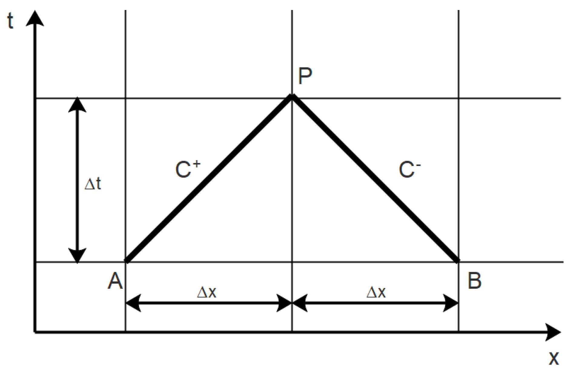
Figure 2.
Effect of m on with .
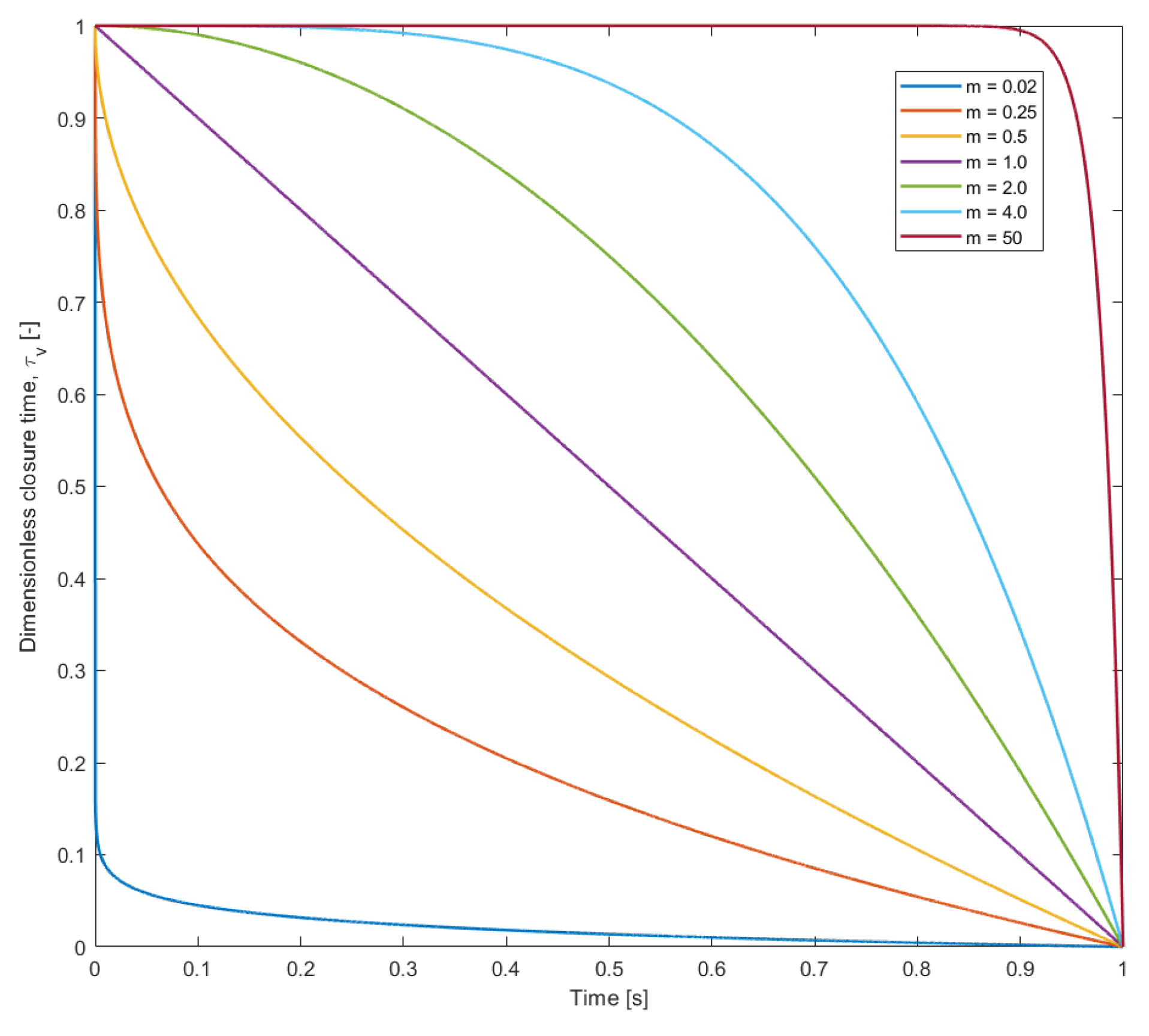
Figure 3.
Grid for two phase Method of Characteristics (MOC).

Figure 4.
Typical experimental setup modelled.

Figure 5.
Comparison of the experimental data (experiment 1 [42]) with the simulated results for each friction model. Note that the steady and quasi-steady friction models gave similar results and all the Convolution Based models (CB) friction models also gave similar results.
Figure 5.
Comparison of the experimental data (experiment 1 [42]) with the simulated results for each friction model. Note that the steady and quasi-steady friction models gave similar results and all the Convolution Based models (CB) friction models also gave similar results.
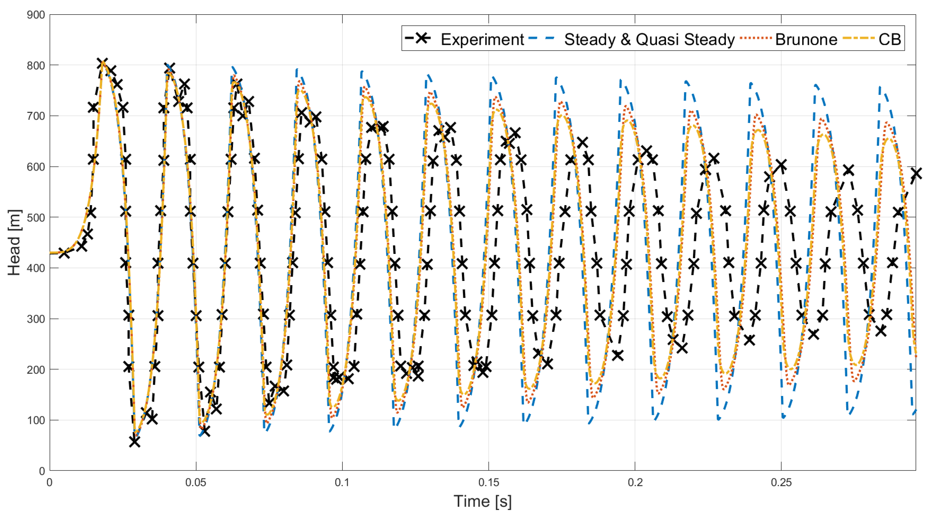
Figure 6.
Comparison of the experimental data (experiment 2 [40])with the simulated results for each friction model. Note that Zielke and Zarzycki friction models gave similar results.
Figure 6.
Comparison of the experimental data (experiment 2 [40])with the simulated results for each friction model. Note that Zielke and Zarzycki friction models gave similar results.
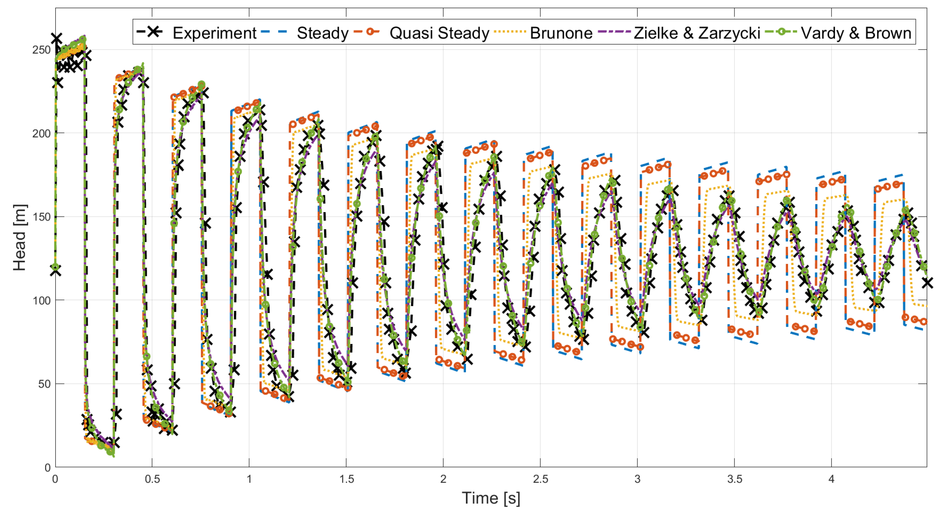
Figure 7.
Comparison of the experimental data (experiment 3 [41]) with the simulated results for each friction model. Note that the steady and quasi-steady friction models gave similar results and all the CB friction models also gave similar results.
Figure 7.
Comparison of the experimental data (experiment 3 [41]) with the simulated results for each friction model. Note that the steady and quasi-steady friction models gave similar results and all the CB friction models also gave similar results.

Figure 8.
Comparison of the experimental data of experiment 4 [41] with the simulated results obtained with the Discrete Vapour Cavity Model (DVCM) and the Discrete Gas Cavity Model (DGCM).
Figure 8.
Comparison of the experimental data of experiment 4 [41] with the simulated results obtained with the Discrete Vapour Cavity Model (DVCM) and the Discrete Gas Cavity Model (DGCM).
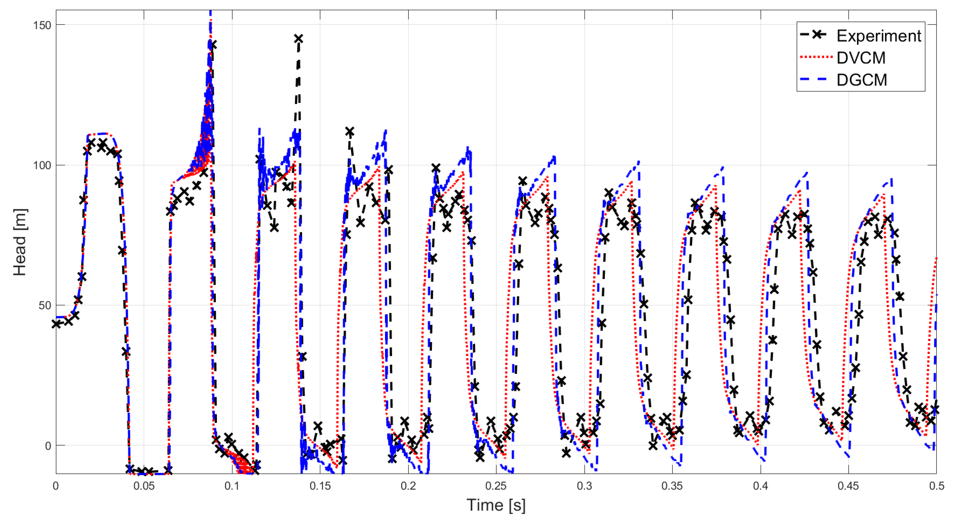
Figure 9.
Comparison of the experimental data of experiment 5 [43] with the simulated results obtained with DVCM and DGCM.
Figure 9.
Comparison of the experimental data of experiment 5 [43] with the simulated results obtained with DVCM and DGCM.

Figure 10.
Comparison of the experimental data of experiment 6 [43] with the simulated results obtained with DGCM.
Figure 10.
Comparison of the experimental data of experiment 6 [43] with the simulated results obtained with DGCM.
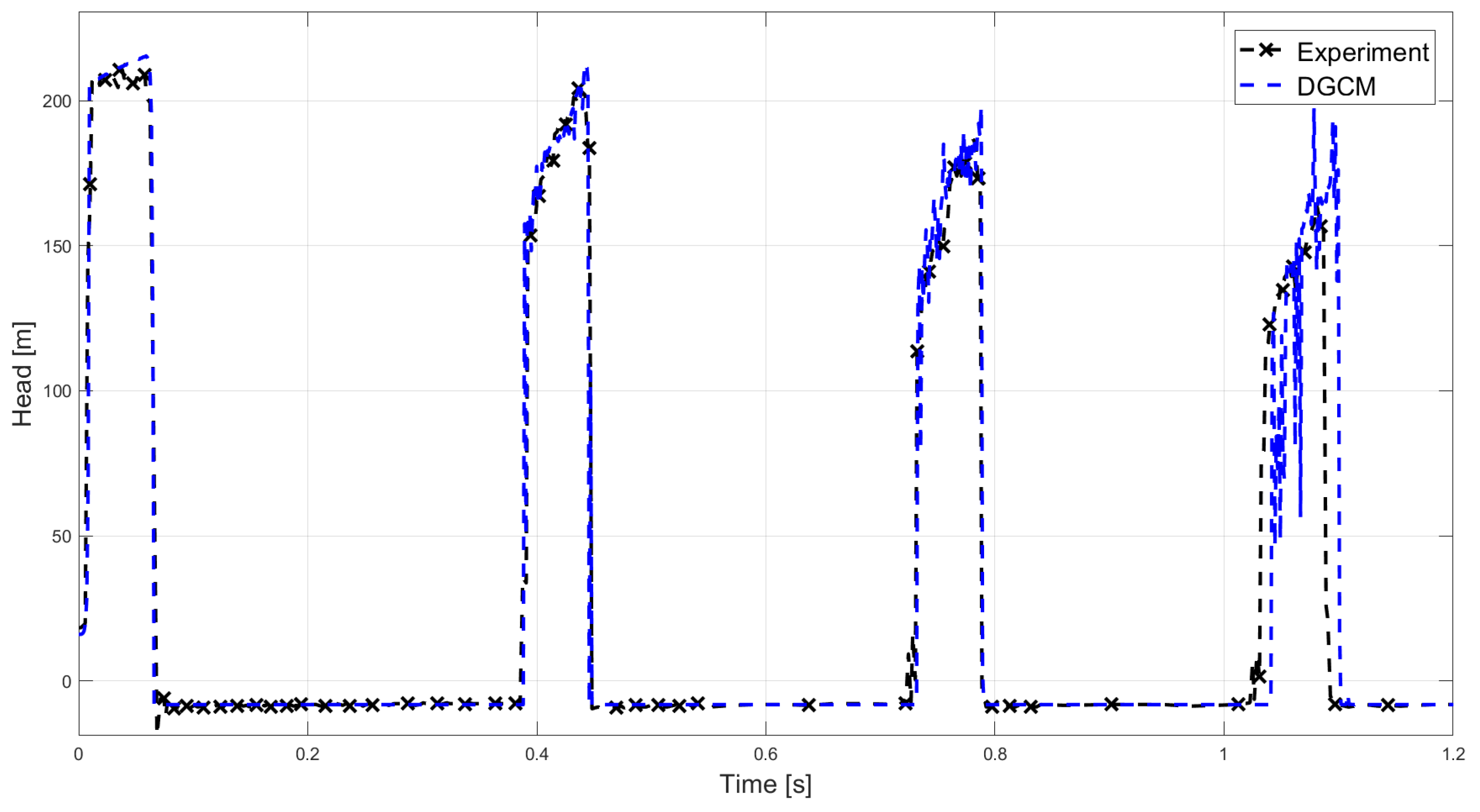

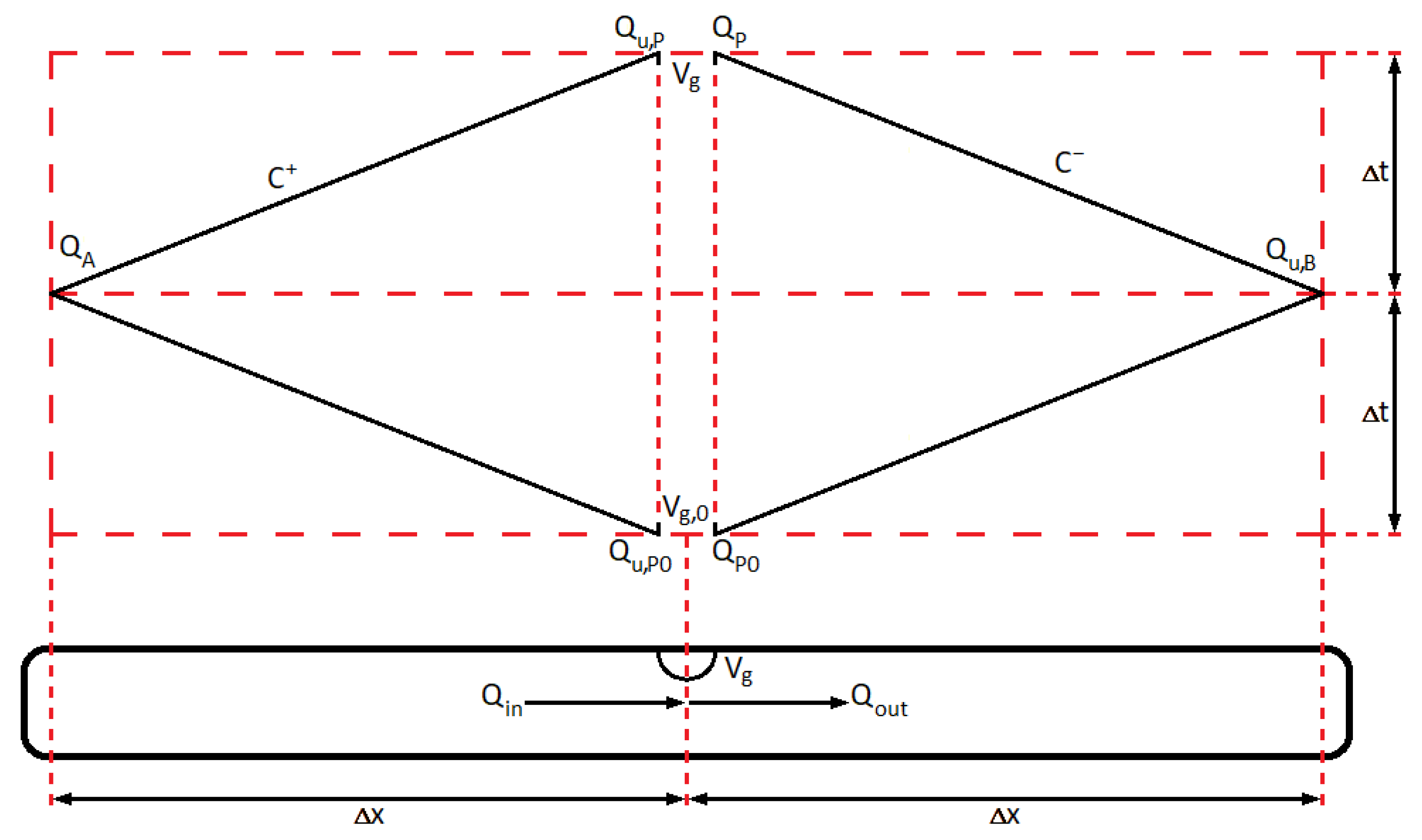
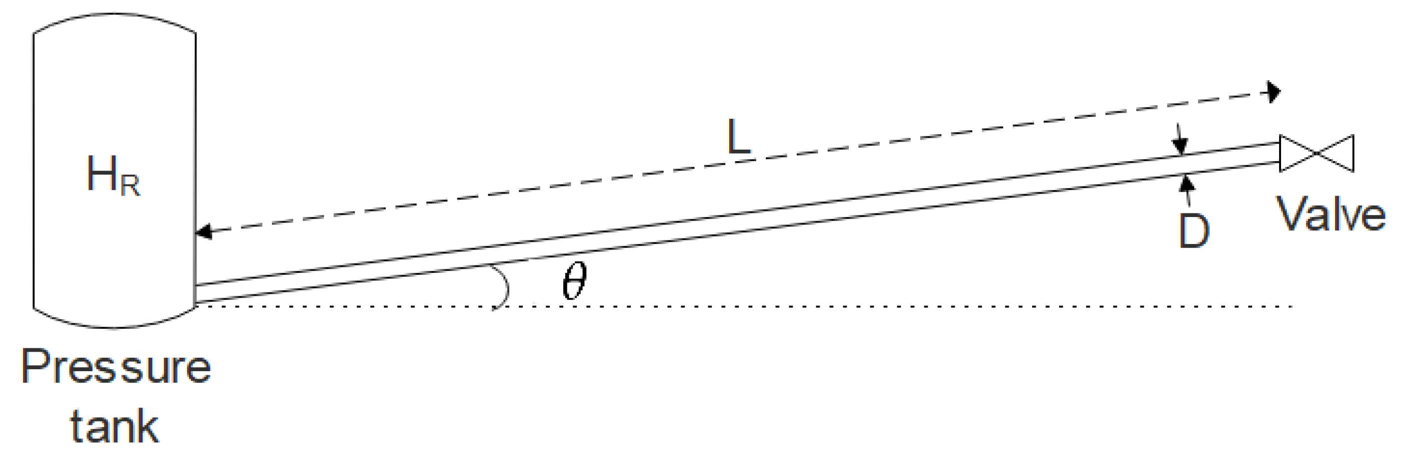
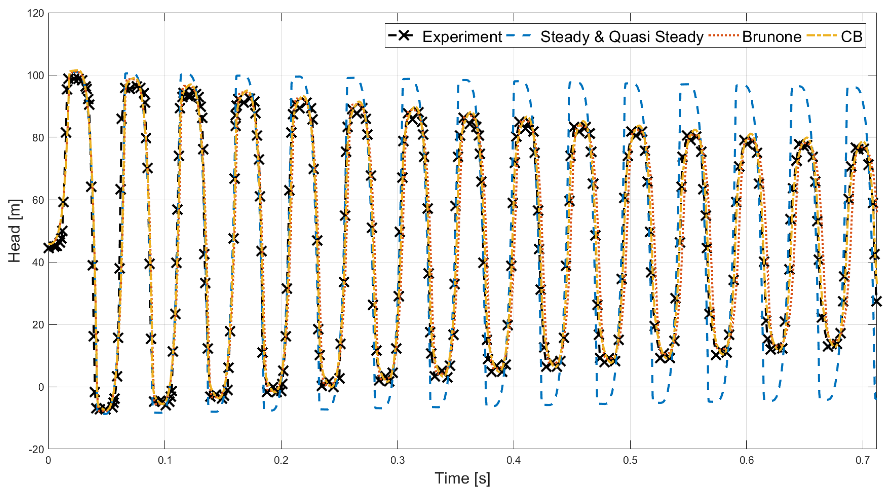
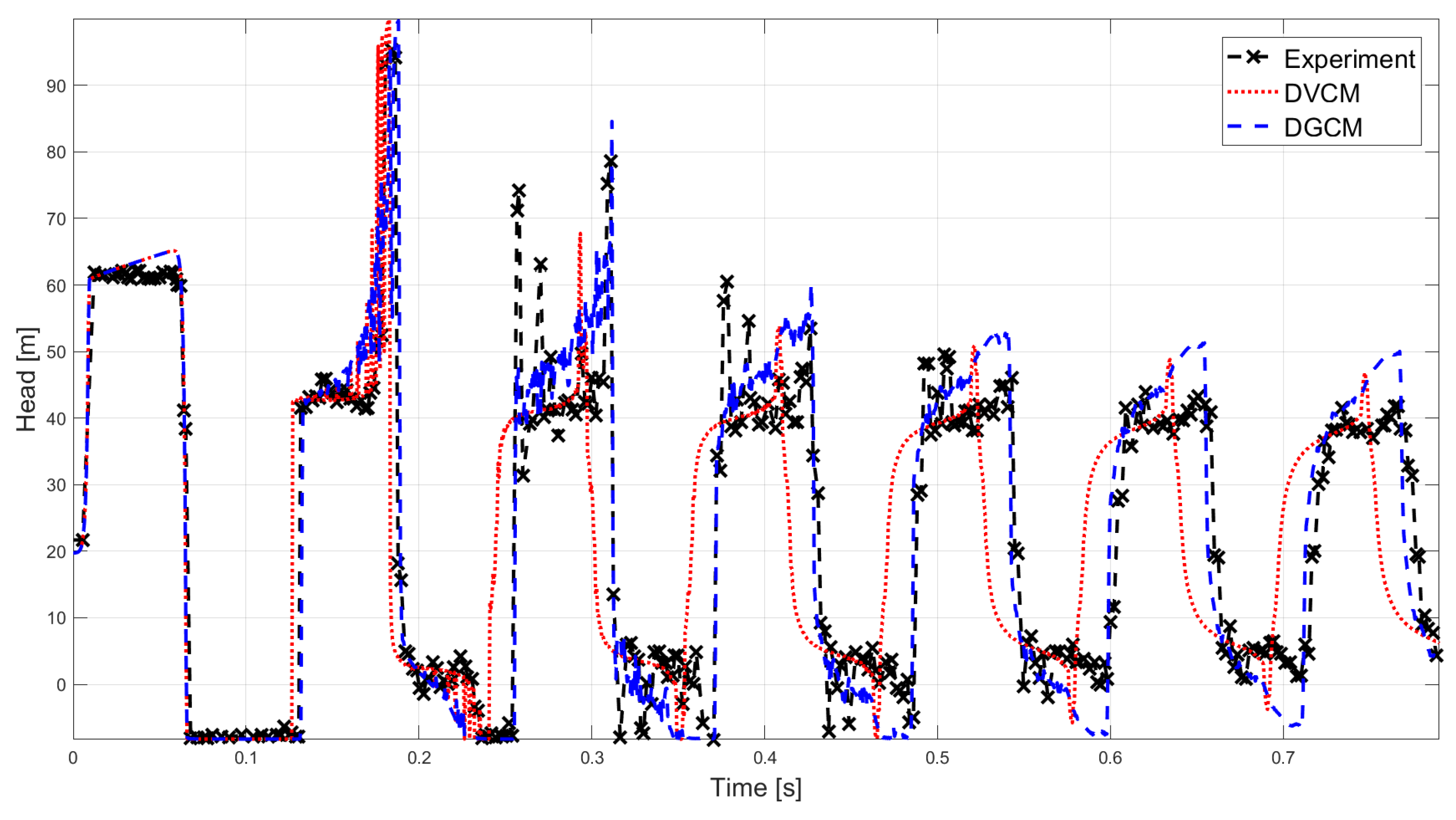
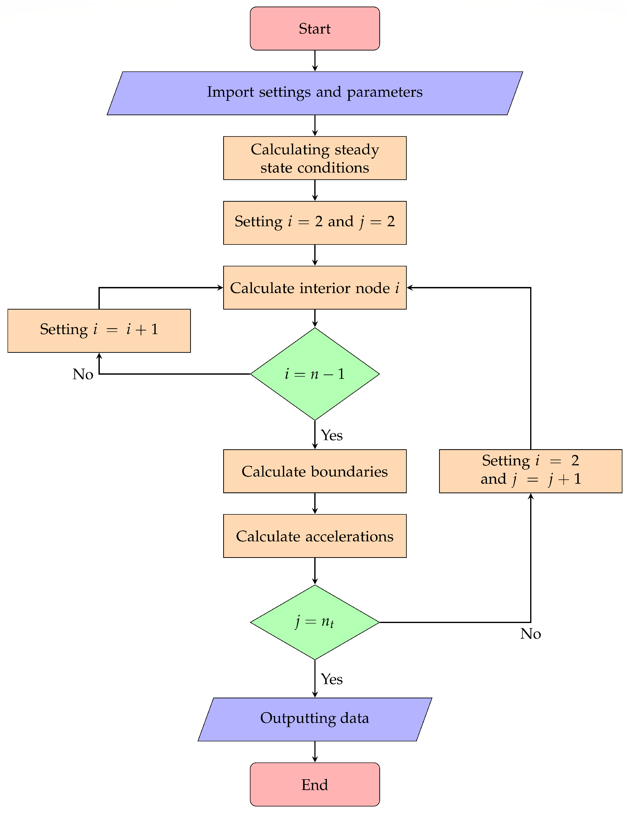
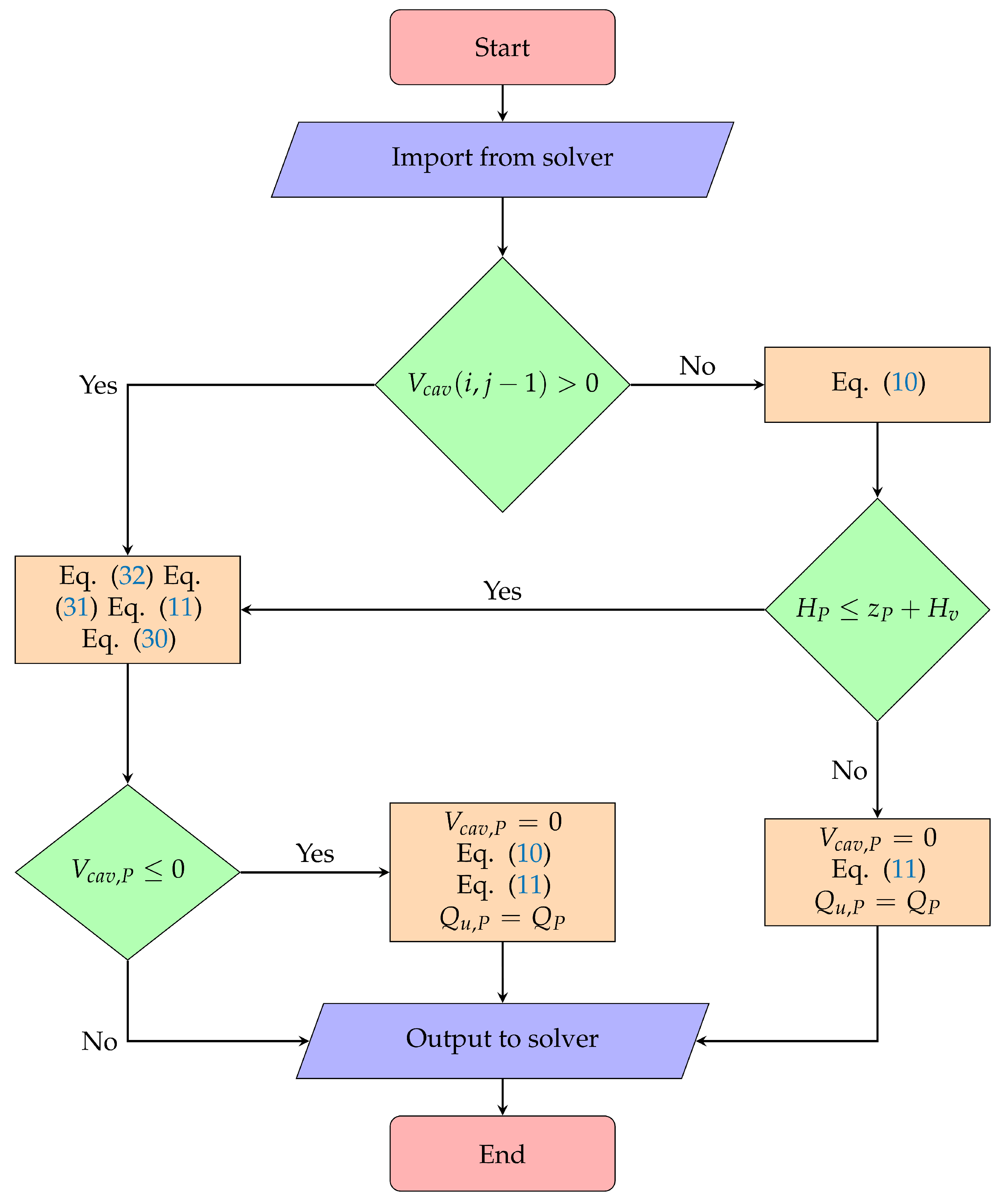
Table 1.
Material and water properties in the simulations.
| Experiment No. | GPa] | m] | mm] | mm] | m] | kg/m] | kg/m· s] | GPa] | m/s] | m/s] | |||
|---|---|---|---|---|---|---|---|---|---|---|---|---|---|
| 1 | 200 | 19 | 1386 | 52052 | |||||||||
| 2 | 120 | 16 | 1 | 1000 | 1282 | 15843 | |||||||
| 3 | 120 | 20 | 1 | 1275 | 8435 | ||||||||
| 4 | 120 | 20 | 1 | 1275 | 9894 | ||||||||
| 5 | 120 | 1319 | 6605 | ||||||||||
| 6 | 120 | 1319 | 30823 |
Table 2.
Comparison of model and experimental results for experiment 1 conducted by [42]. The calculations were conducted on a laptop with an Intel® Core i7-4700MQ processor (Santa Clara, CA, USA) and 8 GB of random access memory (RAM).
Table 2.
Comparison of model and experimental results for experiment 1 conducted by [42]. The calculations were conducted on a laptop with an Intel® Core i7-4700MQ processor (Santa Clara, CA, USA) and 8 GB of random access memory (RAM).
| Parameter | Experiment | Steady | Quasi-Steady | Brunone | Zielke | Vardy & Brown | Zarzycki |
|---|---|---|---|---|---|---|---|
| Oscillation frequency | |||||||
| Maximum head [m] | |||||||
| Deviation from experiment [%] | − | ||||||
| Third pressure peak [m] | |||||||
| Deviation from experiment [%] | − | ||||||
| Tenth pressure peak [m] | |||||||
| Deviation from experiment [%] | − | ||||||
| Calculation time [s] | − | ||||||
| Normalized calculation time [−] | − |
Table 3.
Comparison of model and experimental results for experiment 2 [40].
Table 3.
Comparison of model and experimental results for experiment 2 [40].
| Parameter | Experiment | Steady | Quasi-Steady | Brunone | Zielke | Vardy & Brown | Zarzycki |
|---|---|---|---|---|---|---|---|
| Oscillation frequency | |||||||
| Maximum head [m] | |||||||
| Deviation from experiment [%] | − | ||||||
| Third pressure peak [m] | |||||||
| Deviation from experiment [%] | − | ||||||
| Tenth pressure peak [m] | |||||||
| Deviation from experiment [%] | − | ||||||
| Calculation time [s] | − | ||||||
| Normalized calculation time [−] | − |
Table 4.
Comparison of model and experimental results for experiment 3 [41].
Table 4.
Comparison of model and experimental results for experiment 3 [41].
| Parameter | Experiment | Steady | Quasi-Steady | Brunone | Zielke | Vardy & Brown | Zarzycki |
|---|---|---|---|---|---|---|---|
| Oscillation frequency | |||||||
| Maximum head [m] | |||||||
| Deviation from experiment [%] | − | ||||||
| Third pressure peak [m] | |||||||
| Deviation from experiment [%] | − | ||||||
| Tenth pressure peak [m] | |||||||
| Deviation from experiment [%] | − | ||||||
| Calculation time [s] | − | ||||||
| Normalized calculation time [−] | − |
Table 5.
Comparison of the Discrete Vapour Cavity Model (DVCM), the Discrete Gas Cavity Model (DGCM), and experimental results for experiment 4 [41].
Table 5.
Comparison of the Discrete Vapour Cavity Model (DVCM), the Discrete Gas Cavity Model (DGCM), and experimental results for experiment 4 [41].
| Parameter | Experiment | DVCM | DGCM |
|---|---|---|---|
| Oscillation frequency | |||
| 1st pressure peak [m] | |||
| Deviation [%] | − | ||
| 2nd pressure peak [m] | |||
| Deviation [%] | − | ||
| 3rd pressure peak [m] | |||
| Deviation [%] | − | ||
| 10th pressure peak [m] | |||
| Deviation [%] | − | ||
| Calculation time [s] | − |
Table 6.
Comparison of DVCM, DGCM, and experimental results for experiment 5 [43].
Table 6.
Comparison of DVCM, DGCM, and experimental results for experiment 5 [43].
| Parameter | Experiment | DVCM | DGCM |
|---|---|---|---|
| Oscillation frequency | |||
| 1st pressure peak [m] | |||
| Deviation [%] | − | ||
| 2nd pressure peak [m] | |||
| Deviation [%] | − | ||
| 3rd pressure peak [m] | |||
| Deviation [%] | − | ||
| 7th pressure peak [m] | |||
| Deviation [%] | − | ||
| Calculation time [s] | − |
Table 7.
Comparison of DGCM and experimental results for experiment 6 [43].
Table 7.
Comparison of DGCM and experimental results for experiment 6 [43].
| Parameter | Experiment | DGCM |
|---|---|---|
| Oscillation frequency | ||
| 1st pressure peak [m] | ||
| Deviation [%] | − | |
| 2nd pressure peak [m] | ||
| Deviation [%] | − | |
| 3rd pressure peak [m] | ||
| Deviation [%] | − | |
| 4th pressure peak [m] | ||
| Deviation [%] | − | |
| Calculation time [s] | − |
© 2018 by the authors. Licensee MDPI, Basel, Switzerland. This article is an open access article distributed under the terms and conditions of the Creative Commons Attribution (CC BY) license (http://creativecommons.org/licenses/by/4.0/).
Share and Cite
MDPI and ACS Style
Kjerrumgaard Jensen, R.; Kær Larsen, J.; Lindgren Lassen, K.; Mandø, M.; Andreasen, A. Implementation and Validation of a Free Open Source 1D Water Hammer Code. Fluids 2018, 3, 64. https://doi.org/10.3390/fluids3030064
AMA Style
Kjerrumgaard Jensen R, Kær Larsen J, Lindgren Lassen K, Mandø M, Andreasen A. Implementation and Validation of a Free Open Source 1D Water Hammer Code. Fluids. 2018; 3(3):64. https://doi.org/10.3390/fluids3030064
Chicago/Turabian StyleKjerrumgaard Jensen, Rune, Jesper Kær Larsen, Kasper Lindgren Lassen, Matthias Mandø, and Anders Andreasen. 2018. "Implementation and Validation of a Free Open Source 1D Water Hammer Code" Fluids 3, no. 3: 64. https://doi.org/10.3390/fluids3030064