Optimal Perturbations of an Oceanic Vortex Lens


1
Departamento de Oceanografía Física, Centro de Investigación Científica y de Educación Superior de Ensenada, 22860 Ensenada, Baja California, Mexico
2
Laboratoire d’Océanographie Physique et Spatiale, Ifremer, 29280 Plouzané, France
3
Laboratoire d’Océanographie Physique et Spatiale, Institut Universitaire Européen de la Mer, 29280 Plouzané, France
*
Author to whom correspondence should be addressed.
Fluids 2018, 3(3), 63; https://doi.org/10.3390/fluids3030063
Submission received: 27 June 2018
/
Revised: 8 August 2018
/
Accepted: 15 August 2018
/
Published: 31 August 2018
(This article belongs to the Collection Geophysical Fluid Dynamics)
Abstract
:The stability properties of a vortex lens are studied in the quasi geostrophic (QG) framework using the generalized stability theory. Optimal perturbations are obtained using a tangent linear QG model and its adjoint. Their fine-scale spatial structures are studied in details. Growth rates of optimal perturbations are shown to be extremely sensitive to the time interval of optimization: The most unstable perturbations are found for time intervals of about 3 days, while the growth rates continuously decrease towards the most unstable normal mode, which is reached after about 170 days. The horizontal structure of the optimal perturbations consists of an intense counter-shear spiralling. It is also extremely sensitive to time interval: for short time intervals, the optimal perturbations are made of a broad spectrum of high azimuthal wave numbers. As the time interval increases, only low azimuthal wave numbers are found. The vertical structures of optimal perturbations exhibit strong layering associated with high vertical wave numbers whatever the time interval. However, the latter parameter plays an important role in the width of the vertical spectrum of the perturbation: short time interval perturbations have a narrow vertical spectrum while long time interval perturbations show a broad range of vertical scales. Optimal perturbations were set as initial perturbations of the vortex lens in a fully non linear QG model. It appears that for short time intervals, the perturbations decay after an initial transient growth, while for longer time intervals, the optimal perturbation keeps on growing, quickly leading to a non-linear regime or exciting lower azimuthal modes, consistent with normal mode instability. Very long time intervals simply behave like the most unstable normal mode. The possible impact of optimal perturbations on layering is also discussed.
1. Introduction
1.1. Meddies
Vortex lenses (also known as Intrathermocline Eddies [1] or Submesoscale Coherent Vortices [2]) are interior oceanic eddies. They commonly form in the vicinity of major intermediate water outflows off concentration basins: Meddies in the Mediteranean outflow ([3,4,5] among many), Peddies in the Persian Gulf outflow [6,7,8] or Reddies in the Red sea outflow [9,10], but were also observed in many marginal seas such as the Mediterranean [1], Beaufort [11], Tasman [12] seas or in the Gulf of Mexico [13]. They usually have strong spice signatures as the water they carry is warmer and saltier than the surroundings. The associated density field is characterized by stretched isopycnals near the eddy core and squeezed isopycnals above and below. This results in a baroclinic tripole potential vorticity anomaly (PVA) structure, with a negative PVA core surrounded by two positive PVA lobes [2,14,15,16]. This PVA distribution induces a vertically sheared anticyclonic circulation.
Among all vortex lenses, meddies have without a doubt been the most observed, and are likely the most common both in the literature and in the ocean. The reader can refer to [3,4,5,17,18], for more details on meddies hydrographic and dynamic properties.
Meddies were identified as the principal source of transport of Mediterranean Outflow Water (there after MOW) [3,19]. The mixing of this warm and salty water mass in the North Atlantic has a major climatic impact as it modifies dramatically the basin’s heat and salt content which drives the meridional overturning circulation. The occurrence of layering above and below meddies was identified as a crucial step of the MOW mixing process by lowering the vertical scale of thermohaline anomalies down to a few metres, where vertical mixing becomes important [17,20,21]. Several processes were proposed to explain the formation of such layers around meddies (and vortex lenses in general): Double diffusive processes [22], critical layer instability [21] and tracer stirring [23,24]. In the latter process, the vertical shear of the azimuthal velocity field of meddies generates high vertical wave number variability from any azimuthal variability. Baroclinic instability of meddies was studied by [21,25] and was shown to be a source of azimuthal variability by breaking the vortex symmetry and might therefore play a primary role in the formation of layering, hence the diffusion of the vortex’s thermohaline properties. Baroclinic instability was also shown to be able to split and trigger filamentation of vortex lenses [21,26] and could thus drive the production of small horizontal scales, which would in turn feed the vertical scale cascade through differential advection [24,27,28]. The stability properties of vortex lenses is thus an important topic as they strongly influences the production of small scale variance and possibly favour the mixing of a climatically important water mass.
The linear and non-linear stability of barotropic or surface intensified vortices has been extensively studied from the 70s ([29,30,31] among many). Though the stability of vortex lenses may have received less attention, works from [21,25,26,32] provide valuable information on the normal mode instability of these structures. Meddies are typically unstable to low azimuthal mode perturbations. The most unstable azimuthal modes are sensitive to the meddy’s local Burger number: in the case of wide, strongly baroclinic lenses, baroclinic instability dominates [32] and the lowest azimuthal wave numbers (modes 1 and 2) emerge while for less stratified or taller lenses, higher modes take over (modes 3 and 4), consistent with mixed baroclinic-barotropic instability [25,32,33]. Carton et al. [26] determined that for a typical Burger number (), the Rossby radius was the critical vortex radius above which baroclinic instability dominates over barotropic instability. They also showed that the PVA distribution of the vortex lens had a strong impact on its stability properties. Using idealized PVA profiles based on observed Rossby and Burger numbers, Hua et al. [21] finally showed that a typical meddy would preferentially be baroclinically unstable, with growth rates significantly slower than the vortex rotation period. However, all the aforementioned studies were restricted either to the normal mode linear instability, or to the long term non linear evolution of the vortices.
1.2. Optimal Perturbations
Normal modes only represent a subset of the possible perturbations, and only on particular occasions are they the fastest growing perturbations: Farrell [34] showed that even though the normal modes dominate the long term destabilization of a flow, transient growth of non-normal perturbations at short time scales can be large enough for the disturbances to reach amplitudes where non-linear effects become important before the normal modes emerge. Indeed, while normal modes grow exponentially with time at a constant rate, there may exist other perturbations with faster growth rates during a finite time interval. This notion of time interval is crucial as an optimal perturbation is only optimal for a given finite time. This theory, referred to as the generalized stability theory and further formalized in [35] consists in searching the fastest growing perturbation regardless of any hypothesis on the perturbation’s spatial and temporal structure and will be detailed in Section 2.1. It received much attention in the atmospheric community, and was successfully implemented in data assimilating forecasting models [36,37,38], confirming that at short term, non-modal perturbations grow faster than normal modes and can trigger explosive cyclogenesis.
Though it was less widely spread in the oceanic community, the methods was applied in a QG model of the Gulf Stream [39] showing that in an intense baroclinic oceanic jet, the optimal perturbations are not of the normal mode type, and should then be considered when aiming to describe the stability of coherent oceanic structures. This is particularly true for some flows (such as the Orr flow) that are stable to normal modes and were found to be unstable to non-modal perturbations [40].
The application of the generalized stability theory to the case of coherent vortices was so far almost restricted to very high Rossby number atmospheric structures such as Hurricanes and tornadoes [41,42]. One recent and notable exception to this is the study of non-modal instability of two layer QG baroclinic vortices and its sensitivity to the stratification and PVA distribution by [43]. They showed that slow geostrophic vortices also could be more unstable to non-modal perturbations than to normal modes, but the study was performed in an idealistic 2-layered framework, and could not reveal the detailed spatial structure of the optimal perturbations nor its extreme sensitivity to the time interval.
The present study describes the growth and detailed spatial structure of the optimal perturbations of an oceanic vortex lens and their sensitivity to the chosen time interval using the adjoint methods of [39,44] in a very high resolution QG model. Though several aforementioned studies showed that both stratification and PVA distribution could impact the stability properties of vortex lenses, here, we will restrain ourselves to the realistic and well studied Cauchy-Lorentz vortex profile of [21].
A brief summary of the generalized stability theory and of its application in the QG framework to compute optimal perturbations is described in Section 2.1. Details of the numerics of the model are given in Section 2.2 and a definition of the vortex parameters can be found in Section 2.3. The results are given in Section 3: In Section 3.1, we show the convergence properties of the adjoint methods and describe the obtained optimal perturbations in terms of growth rate, and their dependencies on the time interval. The fine-scale spatial structures of the optimal perturbations are detailed in Section 3.2. In Section 3.3, we show the evolution of the optimal perturbations in a fully non-linear QG model, their effective growth rates and the time evolution of their azimuthal and vertical structures. Finally, these results are summed up and discussed in Section 4
2. Methods
2.1. Adjoint Methods
The theory and methods used here to obtain the optimal perturbations of the vortex lens are entirely based on the work of [39,44] in the QG framework. While we will sum up a brief overview of the methods restricted to optimal perturbations in the sense of energy maximization for time-independent mean flows (autonomous operators) with constant Coriolis parameter and Brünt Väisälä frequency, we strongly recommend the reader to refer to [44,45] for a general and detailed description of the theory and methods along with an inspiring discussion.
In the QG framework, PV (q) relates to the stream function () through the linear operator :
where is the Laplacian operator, z is the vertical coordinate, and f and N are the Coriolis and the Brunt-Váisálá frequencies, respectively.
In the QG model used here, PV evolution reads:
where is a bilaplacian operator associated with the viscosity and J is the Jacobian operator.
When studying the instability of a geophysical flow, one is primarily interested in the influence of initially small disturbances on the flow. It is thus convenient to decompose the variables into a mean, stationary, azimuthally symmetric part and a time-varying perturbation part with and . The latter hypothesis allows to drop the perturbation products in the advection terms of Equation (3) (i.e., the Jacobian operator), yielding to the tangent linear PV evolution equation:
Using (2), one can link the perturbation stream function to its temporal derivative through a single linear operator :
where the primes have been dropped as we will now only consider the perturbation itself.
The operator is associated with a unique propagator that links the solution of (5) at a time to the initial conditions :
To measure the magnitude of a perturbation at time , and thus its growth compared to the initial conditions, it is necessary to define a norm. As discussed by [44,45], the choice of this norm will dramatically impact the structure and growth of the optimal perturbations. A perturbation that is optimal for a given norm will likely not be for another one. Here, we will restrain ourselves to the study of perturbations that maximize the growth of the total energy. In the QG framework, the total energy is defined as:
dropping the factor, we can define a convenient inner product associated with the energy norm:
Using (5), the total energy of the perturbation at time is thus measured by and the amplification factor of the perturbation is:
By definition of the inner product, the adjoint operator of the linear operator and the adjoint propagator of the propagator satisfy:
where is defined as:
The amplification factor at time reads:
and the adjoint of the tangent linear QG model is
Noting that the adjoint of the propagator of a linear operator is the propagator of the adjoint operator, Equations (5) and (16) immediately yield to the propagator and its adjoint and thus an explicit form of the perturbations amplification factors:
The fastest growing (optimal) perturbation is simply the eigenvector associated with the largest eigenvalue of the operator and the growth rate of the optimal perturbation is given by this eigenvalue.
In practice, integrating an initial perturbation in the QG tangent linear model during a time interval is equivalent to computing Equation (5). The model input is and the output . Integrating the latter output as an initial condition in the QG adjoint model is equivalent to computing Equation (16), where the input is and the output is . Following the power method principle [46], iterating the latter operation until a satisfying convergence is obtained is an efficient way of determining the largest eigenvalue and associated eigenvector. The optimal perturbations for a given time interval are thus obtained integrating successively N times the tangent linear and adjoint QG models during this time interval .
In the case of normal modes, the perturbation stream function has the form , where m is the azimuthal wave number, the amplification factor simply reads , where is the growth rate of the perturbation. For the clarity of the discussion, equivalent growth rates will be favoured over amplification factors. The optimal perturbation’s equivalent growth rates are computed as .
2.2. The Numerical Models
The tangent linear and adjoint numerical models are derived from [47]’s pseudo spectral non-linear QG model, which is also used in Section 3.3 to study the non-linear evolution of optimal perturbations. The models are run with horizontal and vertical grid steps of respectively m and m in a doubly periodic 250 km wide and 2400 m deep parallelepipoid domain. The time step is s. The non-linear, tangent linear and adjoint models respectively solve Equations (3), (4) and (16). Time integration of the latter equations requires the inversion of to compute the advection terms (i.e., the Jacobian operators). The model being pseudo spectral, this operation is performed in the Fourier space where integration of the Laplacian falls down to a simple multiplication by the squared wave number. A decomposition into vertical modes is also used. Dissipation is only used at very small scale to avoid numerical instability and is set as small as possible.
2.3. Parameterisation of the Vortex Lens
Throughout this study, we use a Cauchy-Lorentz stream function defined as:
where is a dimensionless intensity parameter, r is the radial coordinate centred at the vortex rotation axis, L is the vortex radius, z is the vertical coordinate and H is the half vortex thickness at the rotation axis. H and L are chosen to satisfy the low local Burger number ( where is the vortex aspect ratio) value typical of meddies (here, ). The Coriolis and Brünt Väisälä frequencies are kept constant with typical Canary basin values: = 8 × 10 s and = 3.2 × 10 s.
3. Results
3.1. Growth Rates of the Optimal Perturbations
Optimal perturbations were computed running iteratively the tangent linear and adjoint models 80 times for a set of time intervals ranging from to days. The growth rates of the perturbations are shown for each iteration in Figure 1a. Convergence of the growth rate is a good indicator that the solution shown really is the optimal perturbation. For short time intervals, the convergence of the solution appears to be much slower than for longer time intervals. For the day and days runs, the solutions don’t seem to have converged after 80 iterations so the optimal perturbation is still not obtained, while 1 iteration is enough for long time interval optimal perturbations to emerge (52 to 174 days). Note however that the meddies simulated here have low Rossby numbers (<0.1), and rotation periods of about 5 days, so that a time scale of 1 or 2 days is likely not in the range where the QG approximation is valid, and these particular cases were only computed as an asymptotic limit of the study.
The slow convergence of the perturbation’s growth rate for small time intervals may be related with their larger azimuthal spectra which will be discussed in Section 3.2. The rate of convergence of the solution is inherently linked to the convergence properties of the power matrix method [46]. In particular, the rate at which the largest eigenvalue will emerge depends on the ratio of the latter and the rest of the spectrum. Namely, if the second largest eigenvalue is much smaller than the largest, convergence is quick, while if they are of comparable magnitude, convergence is slow.
The growth rates of the optimal perturbations after 80 iterations are shown against in Figure 1b. From = 3 to 174 days, decreases with growing from = 2.81 × for days to = 0.55 × for days, converging towards the most unstable normal mode’s growth rate = 0.454 × (discontinuous black line). Note however that the growth rate of optimal perturbations for = 1 and 2 days does not comply with this general decrease of the growth rate with increasing time interval. Several numerical issues may explain this result: The first is the possibility of a non-convergence of the solutions, as the convergence rate was shown to decrease with decreasing time intervals (Figure 1). The model’s viscosity could also play a role in damping quickly the short wavelengths associated with short time intervals. Finally, the Cartesian geometry of the model’s numerics, while the natural coordinates of the vortex are cylindrical, may lead to inhomogeneous numerical discretization errors that could be particularly severe for short azimuthal waves. Note however that, as discussed above, time scales of 1 to 3 days are not of particular interest here, as they lay at the limit of the QG framework’s validity.
3.2. Spatial Structure of the Optimal Perturbations
3.2.1. Horizontal Structure
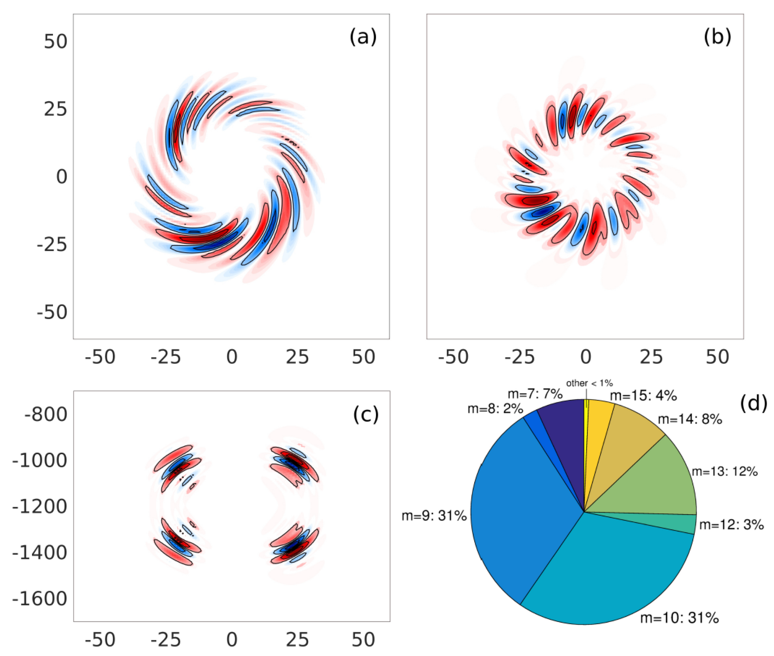
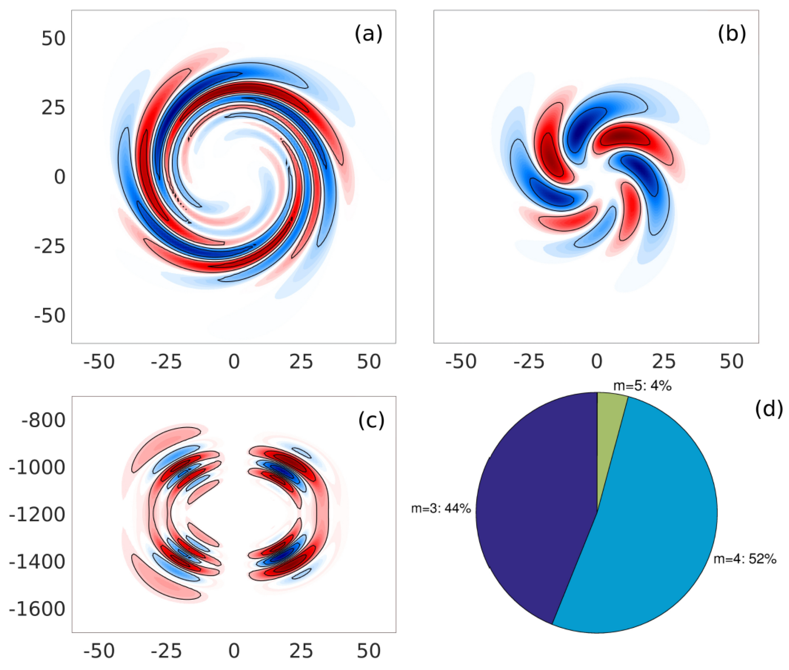
The horizontal structures of the and 174 days optimal perturbations are illustrated respectively in Figure 2, Figure 3, Figure 4 and Figure 5. Panels (a) and (b) show PV sections respectively through the vortex core and lobes.
All 4 examples show intense cyclonic rolling of the perturbation around the vortex core. This spiralling against the mean flow’s velocity shear is similar to that observed by [41,42] for very high Rossby number barotropic vortices. A straightforward comparison can also be made with the results of [40] who showed that optimal perturbations of a linearly sheared parallel flow tend to tilt against the mean shear. This spiralling is much less intense in the vortex lobes, except for long time intervals ( days). The minimum of spiralling is coincident with the minimum of radial shear of azimuthal velocity, suggesting that spiralling could result from the stirring of PV anomalies by the strain field of the mean flow, corresponding to the adjoint advection term in the adjoint model. The increased spiralling for long time intervals supports this hypothesis: the perturbation is advected for a longer time in the adjoint model, resulting in increased stirring.
To describe in details the horizontal structure of optimal perturbations, it is convenient to decompose them as a sum of azimuthal modes and to define the total energy associated with each mode:
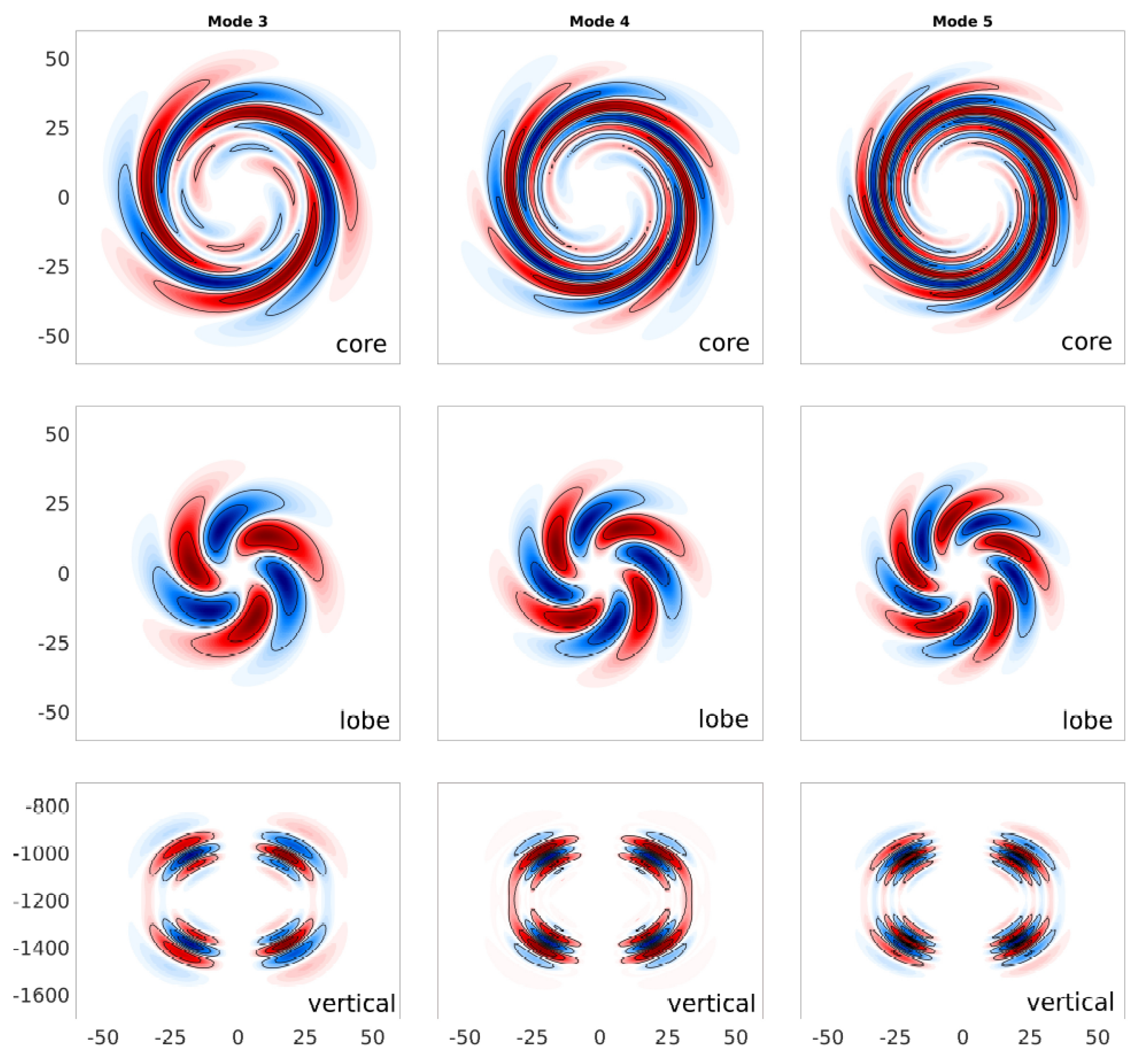
An example of the spatial structure of the azimuthal modes is shown in Figure 6 for the days optimal perturbation. Note that each azimuthal mode has its own vertical structure. The azimuthal energy distribution is shown in detail as pie charts in Figure 2c, Figure 3c, Figure 4c and Figure 5c. It suggests that optimal perturbations can have a variety of azimuthal structures depending on the time interval.
A sensitivity analysis of the azimuthal structure of optimal perturbations was performed for time intervals ranging from 1 to 174 days. Results are shown in Figure 7; panel (a) shows the azimuthal distribution of the optimal perturbation energy for the whole range of time intervals and panel (b) shows the evolution of the energy contribution of each azimuthal mode. For short time intervals, the optimal perturbations are dominated by high azimuthal modes. As increases, the dominant azimuthal modes decrease; for time intervals longer than 52 days, only the mode m = 2 can be found in the optimal perturbation.
The width of the azimuthal spectrum also strongly depends on the time interval: for 3 days, energy is widely spread between modes 10 and 19. As increases, the spectrum becomes narrower, with only three azimuthal modes found in the 17 days optimal perturbation. For time intervals longer than 28 days, the optimal perturbation becomes mono-chromatic, with a transition from azimuthal modes 3 to 2. The range of time intervals in which each azimuthal mode can be found can be inferred from Figure 7b which shows the evolution of each azimuthal mode energy against time interval: high azimuthal modes are only found in narrow ranges of time intervals and as the modes lower, they are found in broader time interval ranges.
3.2.2. Vertical Structure
The vertical structures of the optimal perturbations are shown in panels (c) of Figure 2, Figure 3, Figure 4 and Figure 5. For all time intervals, they show intense PVA layering in the form of a succession of thin PVA anomalies with alternating signs. This layering is concentrated at the edges of the lens and totally absent in the vortex core. This distribution is reminiscent of the typical layering observed with CTD and seismic data around meddies and is strikingly similar to [24]’s results of layering formation from passive tracer advection. This suggests that the layered structure of optimal perturbations could result from the stirring of the perturbation by the vertically sheared mean flow in the adjoint advection operator.
The optimal perturbation was projected onto a base of vertical modes following [47]:
where, in the case of a constant , the vertical modes are defined as:
Figure 8 shows the distribution of energy on the vertical modes for = 4, 10, 17 and 174 days. Because of the vertical symmetry of the vortex, even modes (continuous lines) largely dominate over odd modes (dashed lines). For all time intervals computed, the energy distribution against vertical modes has a bell shape. The spectral peak defined by the maximum of the curve does not seem to have a strong dependence on . In all 4 cases, this peak is centred between vertical modes 26 and 34. However, has a stronger impact on the width of the spectrum: for short time intervals ( = 4 days), the energy is concentrated near vertical mode 30 and the narrow distribution indicates little energy at very low or very high vertical modes. As time interval increases, the spectrum widens, resulting in a more homogeneous distribution of the energy at all vertical scales for the long time intervals ( = 174 days), contrary to the azimuthal distribution which was shown to have a broader spectrum for short time intervals.
3.3. Evolution of the Optimal Perturbations in the Non Linear Model
Optimal perturbations were implemented in the QG non-linear model to assess their impact on the destabilization of a vortex lens in a more realistic framework. The vortex velocity field was initialized as a sum of a mean flow and a perturbation: and then integrated during 70 days. Time evolution of the energy amplification factor is shown on Figure 9a for the = 4, 10, 17 and 174 days optimal perturbations. The days optimal perturbation (yellow line) has an exponential growth, as expected from a normal mode perturbation, confirming that this time interval is long enough for the optimal perturbation to converge towards the most unstable normal mode. This results in a time independent growth rate (Figure 9c), consistent with a normal mode-like exponential amplification.
For shorter time intervals ( = 4, 10 and 17 days), the amplification factor has a clearly different behaviour. In all three cases, it reveals a transient growth of energy during an initial phase, followed by an almost symmetric decay. The time position of the maximum amplification factor grows with : for the = 4 days optimal perturbation, the amplification is maximum at t = 3.4 days, 6.9 days for = 10 days and 11.8 days for = 17 days. The transient growth and decay of the optimal perturbations results in time dependent growth rates. The latter are larger than the time independent normal mode’s growth rate during a finite time. After the amplification factor and the growth rate have reached their maximum, two behaviours arise: for small time intervals ( = 4 and 10 days) the growth of optimal perturbations drops rapidly towards negative growth rates (decay of the perturbation) while the = 17 days optimal perturbation keeps on growing, as its growth rate eventually converges towards the fastest growing normal mode (approximated here by the = 174 days optimal perturbation). Figure 9 also reveals some inconsistencies between the linear and the non-linear results: At time t = 4 days, the time interval = 4 days optimal perturbation does not have the largest amplification factor. Similarly, at t = 10 days, the = 17 days optimal perturbation has grown faster than the = 10 days one. These somehow unexpected results might result from enhanced stirring and mixing of high azimuthal mode (small horizontal scale), yielding rapid dissipation in the fully non-linear model. This could explain why the = 4 and 10 days optimal perturbations, which are made of high azimuthal modes, decay instead of exciting normal modes.
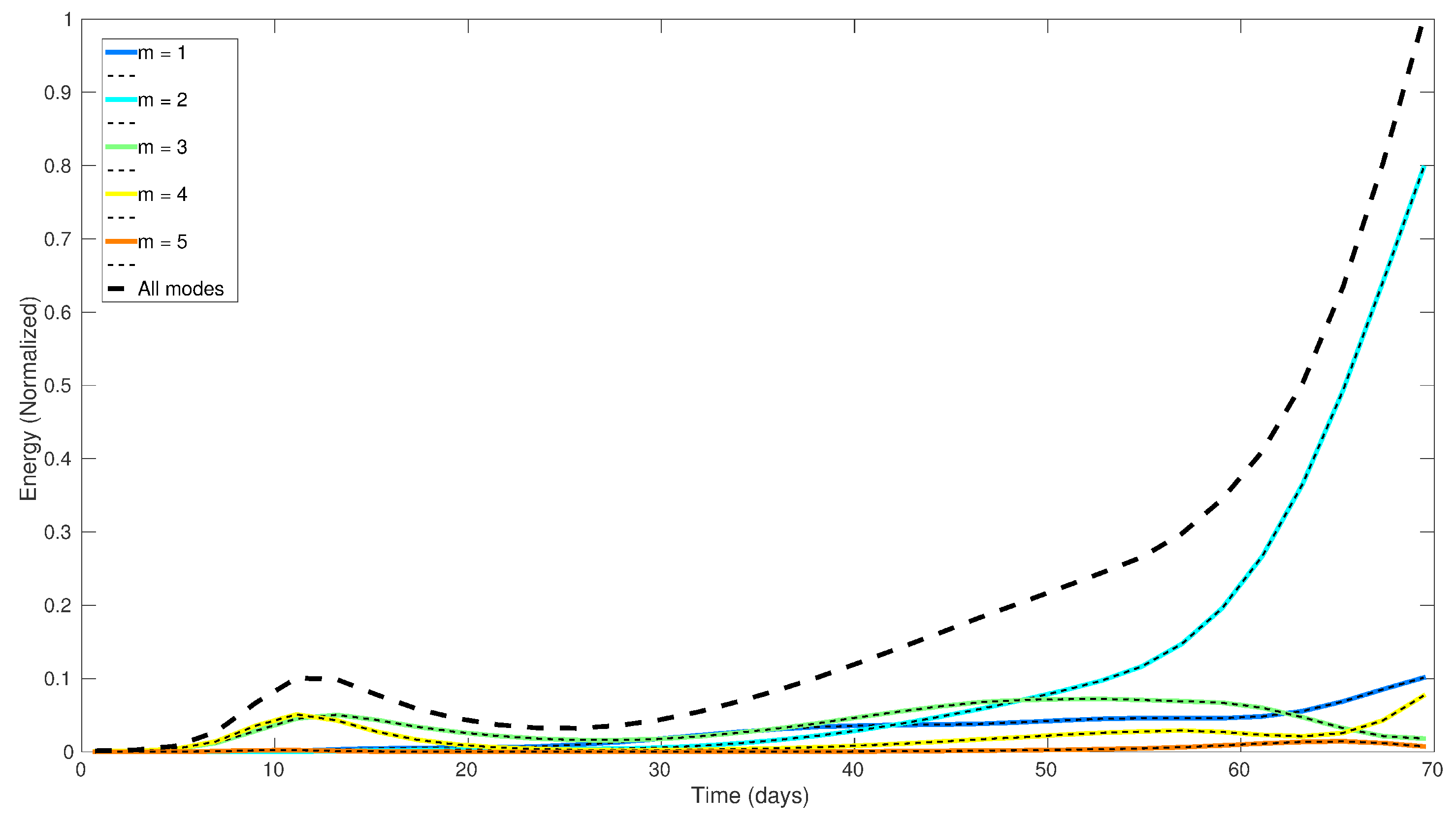
Of the four non-linear runs discussed above, the = 17 days case is of special interest, as it is the only computed non-modal perturbation that does not decay after its transient growth maximum. The non-linear evolution of its spatial structure is shown at t = 0, 17, 40 and 62 days on Figure 10 while the time evolution of the energy of azimuthal modes is shown on Figure 11. The colour scale on each panel of Figure 10 was normalized by its maximum value, and the evolution and growth of energy is to be inferred from Figure 11. After 17 days, the perturbation has started to roll anticyclonically as modes 3 and 4 have grown significantly and dominate over all other modes, in good agreement with the linear predictions. The anticyclonic rolling is accompanied with an increase of the vertical scales of the perturbation, consistent with PV perturbation stirring by the vertically sheared mean azimuthal flow. Indeed, while advection in the adjoint model resulted in a cyclonic stirring, and the formation of small vertical scales, the first 17 days of advection in the direct non linear model first act to undo both the intense horizontal rolling and vertical layering. After 20 days, energy of mode 4 has decayed significantly, contrarily to mode 3. After 40 days, mode 3 triggers spiralling arms at the outer edge of the vortex core, while small satellite vortices start to form in the vortex lobes. Simultaneously, the amplitudes of modes 1 and 2 almost reach that of mode 3. Intense layering starts to form and is obvious on the PVA vertical sections, showing that optimal perturbations can be an efficient way to rapidly trigger an intense vertical cascade. After 62 days, mode 2 has overtaken all other modes and contains nearly 80% of the perturbation energy. Vertical layering has still increased in the vortex lobes. The final emergence of mode 2, accompanied by a convergence of the = 17 days optimal perturbation’s growth rate towards the = 174 days case (Figure 9c) suggests that the normal mode was eventually excited by the non-normal perturbation.
4. Discussion and Summary
In this paper, we studied the optimal perturbations of a vortex lens in the QG framework, their fine-scale azimuthal and vertical structures and their sensitivity to the time interval of optimization . We also investigated their fate in a fully non-linear QG model.
The linear stability analysis revealed that the impact of on optimal perturbation’s growth rates is dramatic for greater than 3 days: The shorter , the larger the growth rate. For short , normal modes are far from being the most unstable ones: the optimal perturbation’s growth rate for days is nearly 5 times larger than that of the most unstable normal mode.
Horizontal structures of optimal perturbations are characterised by an intense counter-shear tilting. Similar results were obtained by [41,42]’s for very high Rossby number barotropic vortices, and by [40] for a parallel shear flow. Here, we suspect that this counter-shear tilting might result from stirring of the perturbation by the adjoint advection terms: in the adjoint model, the relative vorticity sign is opposite to that of the tangent linear model, so that the perturbation is stirred cyclonically around the vortex’s mean flow.
Decomposing the optimal perturbation onto azimuthal modes, we show that the horizontal structures of optimal perturbations also dramatically change with . While the normal mode theory predicts that low Burger number vortex lenses are more unstable to low azimuthal mode perturbations [25,32], our results show that short optimal perturbations are composed of a broad spectrum of high azimuthal wave numbers, suggesting that instability to high wave numbers is not restricted to high Burger number vortices, when considering the full range of possible perturbations. The impact of on the width of the azimuthal spectrum is also obvious: Short optimal perturbations are composed of a broad range of azimuthal modes while for larger , perturbations are nearly monochromatic. This might explain the power matrix method’s slow convergence for very short since [46] showed that the convergence rate depends on the ratio of the largest eigenvalue to the rest of the spectrum.
The vertical structure of optimal perturbations consists of a concentric piling of alternating sign PVA layers. However, the presence of layered patterns in the vertical structure of optimal perturbations should not lead too quickly to the conclusion that non-modal instability could be the origin of the layering observed around meddies. Meunier et al. [24] showed that the vertical shear of a vortex lens’s azimuthal flow produces small scale layered patterns through the stirring of any horizontal tracer anomaly (Temperature, salinity, PV or any conservative tracer). As for the counter-shear tilting observed in the horizontal structure of optimal perturbation, stirring of the PV perturbation by the adjoint advection terms should naturally result in the generation of fine-scale concentric layers such as those observed here.
The vertical structure of optimal perturbations is also sensitive to . Although the latter does not impact the energy maximum, which is always centred between modes 25 and 33, the width of the vertical spectrum increases with decreasing , showing this time that low azimuthal mode perturbations (large ) are composed of a much richer range of vertical scales than high azimuthal modes optimal perturbations.
Initialisation of the non-linear QG model, adding the optimal perturbations to the vortex lens mean flow, illustrates well the transient nature of optimal perturbations, with time-dependent growth rates. Different behaviours arise depending on : for short optimal perturbations, the perturbations decay after an initial phase of growth while for intermediate , the growth rates diminish, but remain positive, so that the perturbation keeps on growing. For very long , where the optimal perturbation is dominated by the azimuthal mode 2 which is close to the fastest growing normal mode, the perturbation grows exponentially (i.e., at a constant growth rate). The observation of negative growth rates associated with the decay of short optimal perturbations might be linked to the length scale of the latter: short optimal perturbations are composed of high azimuthal modes, hence small scale perturbations, which are much more sensitive to the bi-harmonic Laplacian dissipation of the non-linear model. Once the transient growth starts to weaken, dissipation takes over. This increased sensitivity of high wave number perturbations to dissipation might also explain why the growth rates associated with the very short optimal perturbations are weaker than expected.
The intermediate case with days is of particular interest because the optimal perturbation does not decay, and the amplification of the optimal perturbation is sufficiently rapid to reach a non linear regime before the most unstable normal mode (m = 2) emerges. In this particular case, it results in the fast growth of an azimuthal mode 3 perturbation which dominates the vortex destabilization and the transition towards a non-linear stage and the formation of spiralling arms eventually detaching into satellite vortices. This suggests that optimal perturbations may impact the long term non-linear evolution of a vortex lens only for certain range of : if is too short, the growth rate is large, but the spatial scale of the perturbation is small and subject to rapid mixing. If is too large, the optimal perturbation is closely resembling the fastest growing normal mode and the latter will emerge quickly and dominate the destabilization process. But for intermediate , the rapid growth of the perturbation quickly modifies the mean flow so that it may become unstable to different perturbations. The possibility for secondary instability to develop on a mean flow that was first destabilized by a primary perturbation would be an interesting follow-up for the present study. Such processes were shown to impact significantly inertia-gravity waves [48], and may also impact oceanic vortices.
The possible impact of optimal perturbations on the formation of layering around meddies remains modest: Hua et al. [21], Meunier et al. [24] showed that baroclinic instability was an efficient process in generating layers, because it breaks the vortex’s axisymmetry, hence providing the necessary azimuthal variability that is transformed into vertical variability by stirring effects; even though optimal perturbations may break this axisymmetry faster than normal modes, and provide higher horizontal wave number variability, that accelerate the vertical variance cascade [27], the long term evolution does not change drastically as in both cases, the same stirring processes will be at work.
Author Contributions
T.M.: Conceptualization, formal analysis, investigation, visualization and writing—original draft; C.M.: Project administration, funding acquisition and writing—review and editing; X.C.: writing—review and editing; S.L.G.: Methodology, software; R.S.: writing—review and editing.
Funding
This work was supported by the SIMILA (SIMI 5-6, 2011) and OLA (PDOC 2011) projects granted by the French National Agency for Research (ANR). T. Meunier is currently funded by a grant from the National Council of Science and Technology of Mexico—Mexican Ministry of Energy—Hydrocarbon Trust, project 201441, which is a contribution of the Gulf of Mexico Research Consortium (CIGoM).
Acknowledgments
This study, as part of the OLA project, was initiated and led by B. Lien Hua, who died on 26 November 2012. The authors, who started working under her supervision, wish to dedicate this paper to her memory, hoping that it would suit her expectations.
Conflicts of Interest
The authors declare no conflict of interest. The founding sponsors had no role in the design of the study; in the collection, analyses, or interpretation of data; in the writing of the manuscript, and in the decision to publish the results.
References
- Dugan, J.P.; Mied, R.P.; Mignerey, P.C.; Schuetz, A.F. Compact, intrathermocline eddies in the Sargasso Sea. J. Geophys. Res. 1982, 87, 385–393. [Google Scholar] [CrossRef]
- McWilliams, J.C. Submesoscale, Coherent Vortices in the Ocean. Rev. Geophys. 1985, 23, 165. [Google Scholar] [CrossRef]
- Armi, L.; Zenk, W. Large lenses of highly saline Mediterranean water. J. Phys. Oceanogr. 1984, 14, 1560–1576. [Google Scholar] [CrossRef]
- Rossby, T. Five drifters in a Mediterranean salt lens. Deep Sea Res. Part A Oceanogr. Res. Pap. 1988, 35, 1653–1663. [Google Scholar] [CrossRef]
- Pingree, R.D.; Le Cann, B. Structure of a meddy (Bobby 92) southeast of the Azores. Deep Sea Res. Part I Oceanogr. Res. Pap. 1993, 40, 2077–2103. [Google Scholar] [CrossRef]
- Senjyu, T.; Ishimaru, T.; Matsuyama, M.; Koike, Y. High salinity lens from the Strait of Hormuz. In Offshore Environments of the ROPME after the War Related Oil-Spill; Terra Scientific Publishing Company: Tokyo, Japan, 1998; pp. 35–48. [Google Scholar]
- L’Hégaret, P.; Lacour, L.; Carton, X.; Roullet, G.; Baraille, R.; Corréard, S. A seasonal dipolar eddy near Ras Al Hamra (Sea of Oman). Ocean Dyn. 2013, 63, 633–659. [Google Scholar] [CrossRef]
- L’Hégaret, P.; Carton, X.; Louazel, S.; Boutin, G. Mesoscale eddies and submesoscale structures of Persian Gulf Water off the Omani coast in spring 2011. Ocean Sci. 2016, 12, 687–701. [Google Scholar] [CrossRef]
- Shapiro, G.I.; Meschanov, S.L. Distribution and spreading of Red Sea Water and salt lens formation in the northwest Indian Ocean. Deep Sea Res. Part A Oceanogr. Res. Pap. 1991, 38, 21–34. [Google Scholar] [CrossRef]
- Meschanov, S.L.; Shapiro, G.I. A young lens of Red Sea Water in the Arabian Sea. Deep Sea Res. Part I Oceanogr. Res. Pap. 1998, 45, 1–13. [Google Scholar] [CrossRef]
- D’Asaro, E.A. Generation of submesoscale vortices: A new mechanism. J. Geophys. Res. 1988, 93, 6685–6693. [Google Scholar] [CrossRef]
- Baird, M.E.; Ridgway, K.R. The southward transport of sub-mesoscale lenses of Bass Strait Water in the centre of anti-cyclonic mesoscale eddies. Geophys. Res. Lett. 2012, 39, L02603. [Google Scholar] [CrossRef]
- Meunier, T.; Tenreiro, M.; Pallàs-Sanz, E.; Ochoa, J.; Ruiz-Angulo, A.; Portela, E.S.C.; Damien, P.; Carton, X. Intra-Thermocline Eddies Embedded within an Anticyclonic Vortex Ring. Geophys. Res. Lett. 2018. [Google Scholar] [CrossRef]
- Morel, Y.; McWilliams, J. Effects of Isopycnal and Diapycnal Mixing on the Stability of Oceanic Currents. J. Phys. Oceanogr. 2001, 31, 2280–2296. [Google Scholar] [CrossRef]
- Carton, X.; Chérubin, L.; Paillet, J.; Morel, Y.; Serpette, A.; Le Cann, B. Meddy coupling with a deep cyclone in the Gulf of Cadiz. J. Mar. Syst. 2002, 32, 13–42. [Google Scholar] [CrossRef]
- Paillet, J.; Le Cann, B.; Carton, X.; Morel, Y.; Serpette, A. Dynamics and evolution of a northern meddy. J. Phys. Oceanogr. 2002, 32, 55–79. [Google Scholar] [CrossRef]
- Ruddick, B.; Hebert, D. The mixing of meddy “sharon”. In Small-Scale Turbulence and Mixing in the Ocean; Elsevier: New York, NY, USA, 1988; Volume 46, pp. 249–261. [Google Scholar]
- Armi, L.; Hebert, D.; Oakey, N.; Price, J.F.; Richardson, P.L.; Rossby, H.T.; Ruddick, B. Two years in the life of a Mediterranean salt lens. J. Phys. Oceanogr. 1989, 19, 354–370. [Google Scholar] [CrossRef]
- Schultz-Tokos, K.; Rossby, T. Kinematics and Dynamics of a Mediterranean Salt Lens. J. Phys. Oceanogr. 1991, 21, 879–892. [Google Scholar] [CrossRef] [Green Version]
- Biescas, B.; Sallarès, V.; Pelegrí, J.L.; Machín, F.; Carbonell, R.; Buffett, G.; Dañobeitia, J.J.; Calahorrano, A. Imaging meddy finestructure using multichannel seismic reflection data. Geophys. Res. Lett. 2008, 35, 11609. [Google Scholar] [CrossRef]
- Hua, B.L.; Ménesguen, C.; Le Gentil, S.; Schopp, R.; Marsset, B.; Aiki, H. Layering and turbulence surrounding an anticyclonic oceanic vortex: In Situ observations and quasi-geostrophic numerical simulations. J. Fluid Mech. 2013, 731, 418–442. [Google Scholar] [CrossRef]
- Ruddick, B. Intrusive mixing in a Mediterranean salt lens-intrusion slopes and dynamical mechanisms. J. Phys. Oceanogr. 1992, 22, 1274–1285. [Google Scholar] [CrossRef]
- Song, H.; Pinheiro, L.M.; Ruddick, B.; Teixeira, F.C. Meddy, spiral arms, and mixing mechanisms viewed by seismic imaging in the Tagus Abyssal Plain (SW Iberia). J. Mar. Res. 2011, 69, 4–6. [Google Scholar] [CrossRef]
- Meunier, T.; Ménesguen, C.; Schopp, R.; Le Gentil, S. Tracer Stirring around a Meddy: The Formation of Layering. J. Phys. Oceanogr. 2015, 45, 407–423. [Google Scholar] [CrossRef]
- Nguyen, H.Y.; Hua, B.L.; Schopp, R.; Carton, X. Slow quasigeostrophic unstable modes of a lens vortex in a continuously stratified flow. Geophys. Astrophys. Fluid Dyn. 2012, 106, 305–319. [Google Scholar] [CrossRef]
- Carton, X.; Sokolovskiy, M.; Ménesguen, C.; Aguiar, A.; Meunier, T. Vortex stability in a multi-layer quasi-geostrophic model: Application to Mediterranean Water eddies. Fluid Dyn. Res. 2014, 46, 061401. [Google Scholar] [CrossRef]
- Haynes, P.; Anglade, J. The vertical-scale cascade in atmospheric tracers due to large-scale differential advection. J. Atmos. Sci. 1997, 54, 1121–1136. [Google Scholar] [CrossRef]
- Klein, P.; Treguier, A.M.; Hua, B.L. Three-dimensional stirring of thermohaline fronts. J. Mar. Res. 1998, 56, 589–612. [Google Scholar] [CrossRef]
- Flierl, G.R. Models of vertical structure and the calibration of two-layer models. Dyn. Atmos. Oceans 1978, 2, 341–381. [Google Scholar] [CrossRef]
- McWilliams, J.C.; Flierl, G.R. On the evolution of isolated, nonlinear vortices. J. Phys. Oceanogr. 1979, 9, 1155–1182. [Google Scholar] [CrossRef]
- Carton, X.J. On the merger of shielded vortices. Europhys. Lett. 1992, 18, 697. [Google Scholar] [CrossRef]
- McWilliams, J.C.; Gent, P.R. The evolution of sub-mesoscale, coherent vortices on the -plane. Geophys. Astrophys. Fluid Dyn. 1986, 35, 235–255. [Google Scholar] [CrossRef]
- Yim, E.; Billant, P. On the mechanism of the Gent-McWilliams instability of a columnar vortex in stratified rotating fluids. J. Fluid Mech. 2015, 780, 5–44. [Google Scholar] [CrossRef] [Green Version]
- Farrell, B.F. The Initial Growth of Disturbances in a Baroclinic Flow. J. Atmos. Sci. 1982, 39, 1663–1686. [Google Scholar] [CrossRef] [Green Version]
- Farrell, B.F.; Ioannou, P.J. Generalized Stability Theory. Part I: Autonomous Operators. J. Atmos. Sci. 1996, 53, 2025–2040. [Google Scholar] [CrossRef] [Green Version]
- Talagrand, O.; Courtier, P. Variational assimilation of meteorological observations with the adjoint vorticity equation. I: Theory. Q. J. R. Meteorol. Soc. 1987, 113, 1311–1328. [Google Scholar] [CrossRef]
- Buizza, R.; Tribbia, J.; Molteni, F.; Palmer, T. Computation of optimal unstable structures for a numerical weather prediction model. Tellus Ser. A 1993, 45, 388. [Google Scholar] [CrossRef]
- Hartmann, D.L.; Buizza, R.; Palmer, T.N. Singular Vectors: The Effect of Spatial Scale on Linear Growth of Disturbances. J. Atmos. Sci. 1995, 52, 3885–3894. [Google Scholar] [CrossRef] [Green Version]
- Moore, A.M.; Farrell, B.F. Rapid Perturbation Growth on Spatially and Temporally Varying Oceanic Flows Determined Using an Adjoint Method: Application to the Gulf Stream. J. Phys. Oceanogr. 1993, 23, 1682–1702. [Google Scholar] [CrossRef] [Green Version]
- Rivière, G.; Hua, B.L.; Klein, P. Influence of the β-effect on non-modal baroclinic instability. Q. J. R. Meteorol. Soc. 2001, 127, 1375–1388. [Google Scholar] [CrossRef]
- Nolan, D.S.; Farrell, B.F. Generalized Stability Analyses of Asymmetric Disturbances in One- and Two-Celled Vortices Maintained by Radial Inflow. J. Atmos. Sci. 1999, 56, 1282–1307. [Google Scholar] [CrossRef]
- Yamaguchi, M.; Nolan, D.S.; Iskandarani, M.; Majumdar, S.J.; Peng, M.S.; Reynolds, C.A. Singular Vectors for Tropical Cyclone-Like Vortices in a Nondivergent Barotropic Framework. J. Atmos. Sci. 2011, 68, 2273–2291. [Google Scholar] [CrossRef]
- Carton, X.; Flierl, G.R.; Perrot, X.; Meunier, T.; Sokolovskiy, M.A. Explosive instability of geostrophic vortices. Part 1: Baroclinic instability. Theor. Comput. Fluid Dyn. 2010, 24, 125–130. [Google Scholar] [CrossRef]
- Farrell, B.F.; Moore, A.M. An Adjoint Method for Obtaining the Most Rapidly Growing Perturbation to Oceanic Flows. J. Phys. Oceanogr. 1992, 22, 338. [Google Scholar] [CrossRef]
- Farrell, B.F. Optimal Excitation of Baroclinic Waves. J. Atmos. Sci. 1989, 46, 1193–1206. [Google Scholar] [CrossRef] [Green Version]
- Gubernatis, J.E.; Booth, T.E. Multiple extremal eigenpairs by the power method. J. Comput. Phys. 2008, 227, 8508–8522. [Google Scholar] [CrossRef] [Green Version]
- Hua, B.L.; Haidvogel, D.B. Numerical simulations of the vertical structure of quasi-geostrophic turbulence. J. Atmos. Sci. 1986, 43, 2923–2936. [Google Scholar] [CrossRef]
- Fruman, M.; Achatz, U. Secondary instabilities in breaking inertia-gravity waves. In Proceedings of the EGU General Assembly Conference Abstracts, Vienna, Austria, 2–7 May 2010; Volume 12, p. 10232. [Google Scholar]
Figure 1.
(a) Growth rate of the perturbation () against the number of iteration through the tangent linear and adjoint models for different time intervals . The additional discontinuous black line represents the growth rate of the most unstable normal mode (). (b) Growth rate of the optimal perturbation against time interval after convergence of the solution (80 iterations through the tangent linear and adjoint models). The discontinuous black line represents the growth rate of the most unstable normal mode ().
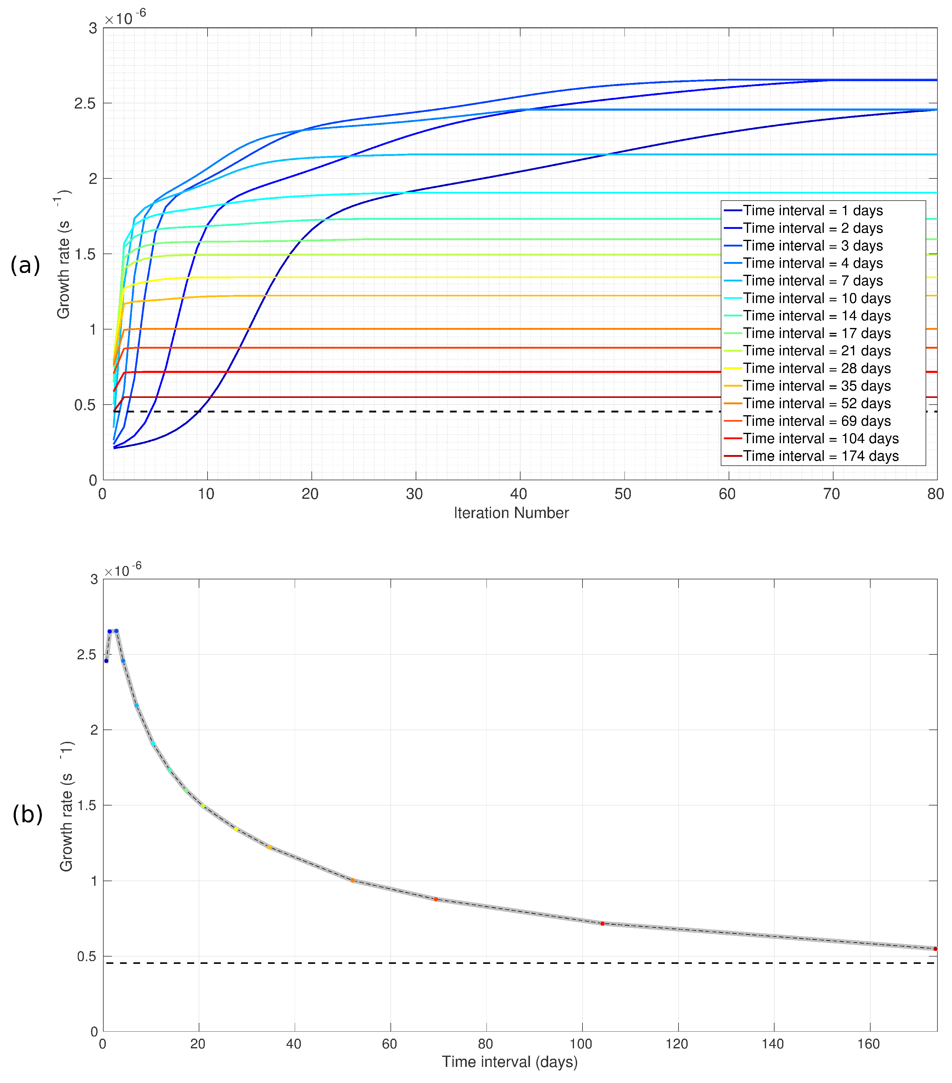
Figure 2.
Optimal perturbation for the time interval = 4 days. (a) PVA horizontal section through the vortex core. (b) PVA section through the vortex lobes. (c) PVA vertical section. (d) Energy distribution on the azimuthal modes.
Figure 2.
Optimal perturbation for the time interval = 4 days. (a) PVA horizontal section through the vortex core. (b) PVA section through the vortex lobes. (c) PVA vertical section. (d) Energy distribution on the azimuthal modes.

Figure 3.
Optimal perturbation for the time interval = 10 days. (a) PVA horizontal section through the vortex core. (b) PVA section through the vortex lobes. (c) PVA vertical section. (d) Energy distribution on the azimuthal modes.
Figure 3.
Optimal perturbation for the time interval = 10 days. (a) PVA horizontal section through the vortex core. (b) PVA section through the vortex lobes. (c) PVA vertical section. (d) Energy distribution on the azimuthal modes.

Figure 4.
Optimal perturbation for the time interval = 17 days. (a) PVA horizontal section through the vortex core. (b) PVA section through the vortex lobes. (c) PVA vertical section. (d) Energy distribution on the azimuthal modes.
Figure 4.
Optimal perturbation for the time interval = 17 days. (a) PVA horizontal section through the vortex core. (b) PVA section through the vortex lobes. (c) PVA vertical section. (d) Energy distribution on the azimuthal modes.

Figure 5.
Optimal perturbation for the time interval = 174 days. (a) PVA horizontal section through the vortex core. (b) PVA section through the vortex lobes. (c) PVA vertical section. (d) Energy distribution on the azimuthal modes.
Figure 5.
Optimal perturbation for the time interval = 174 days. (a) PVA horizontal section through the vortex core. (b) PVA section through the vortex lobes. (c) PVA vertical section. (d) Energy distribution on the azimuthal modes.

Figure 6.
Projection of the optimal perturbation for the time interval = 17 days on the 3 most energetic azimuthal modes (m = 3, 4, 5). The top panels show PVA horizontal sections through the vortex core; the middle panels show PVA horizontal sections through the vortex lobes and the bottom panels show PVA vertical sections.

Figure 7.
(a) Distribution of the perturbation energy on the 20 first azimuthal modes for time intervals ranging from 1 to 174 days. For short time intervals, the spectrum is broad and high wave numbers dominate. As the time interval increases, the spectrum becomes narrower and low azimuthal modes dominate. (b) Relative energy of the azimuthal wave numbers against time interval . (Energy of each mode normalized by the total energy of the optimal perturbation for each computed time interval). Each azimuthal mode occupies a specific time interval band. High azimuthal modes occupy narrow time interval bands overlapping one another while low azimuthal modes occupy larger time interval bands.
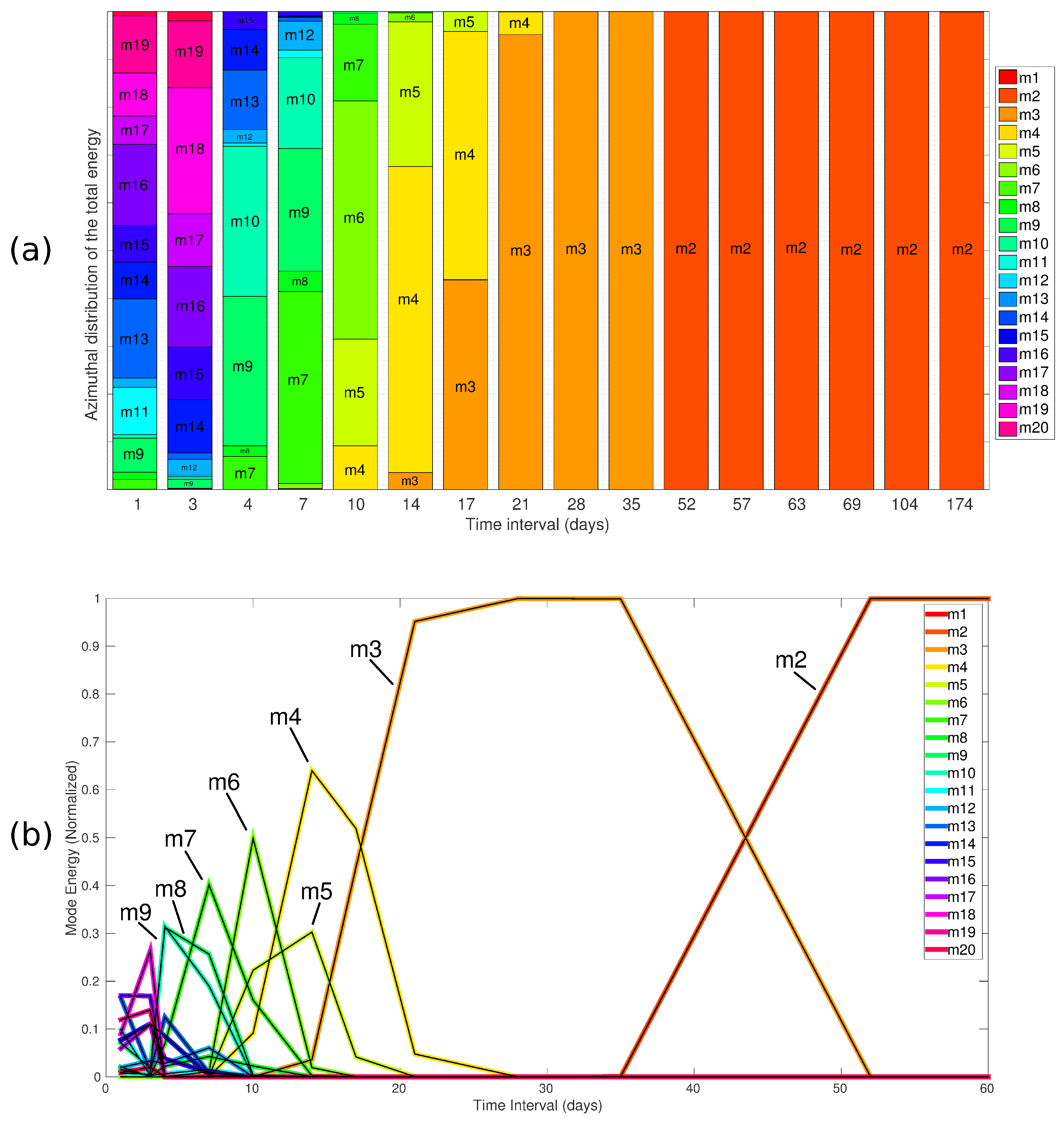
Figure 8.
Energy distribution on the vertical modes of the optimal perturbations for time intervals = 4, 10, 17 and 174 days (Energy of each vertical mode normalized by the total perturbation energy). As an effect of the vertical symmetry of the vortex lens, even modes have much more energy than odd modes. Whereas the time interval does not have a clear effect on the most energetic vertical modes (centre of the spectral peak), it clearly affects the width of the spectral peak. The longer the time interval, the wider the energy spectrum.
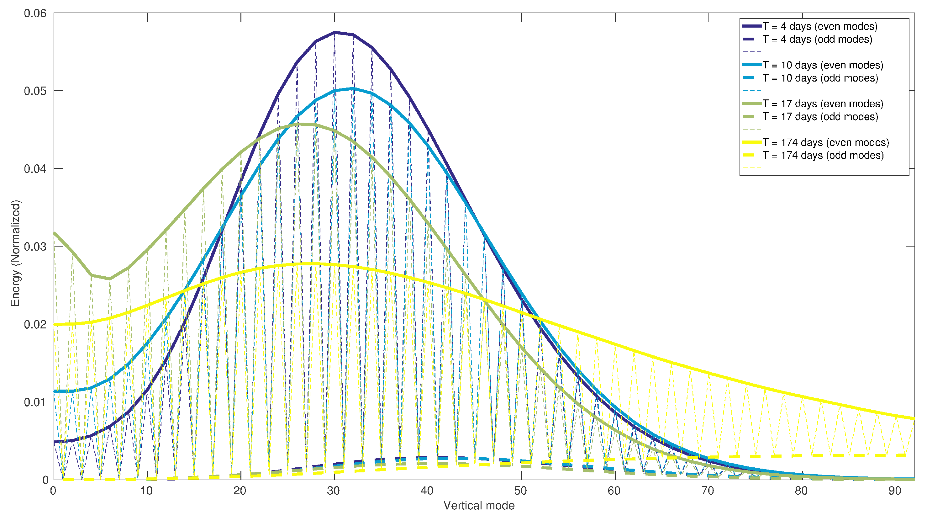
Figure 9.
Time evolution of the optimal perturbations for time intervals = 4, 10, 17 and 174 days implemented in the non-linear QG model. (a) Amplification factor (non-dimensional) against time (days); (b) Zoom of (a) between 0 and 25 days; (c) Growth rate (s) against time(days).
Figure 9.
Time evolution of the optimal perturbations for time intervals = 4, 10, 17 and 174 days implemented in the non-linear QG model. (a) Amplification factor (non-dimensional) against time (days); (b) Zoom of (a) between 0 and 25 days; (c) Growth rate (s) against time(days).

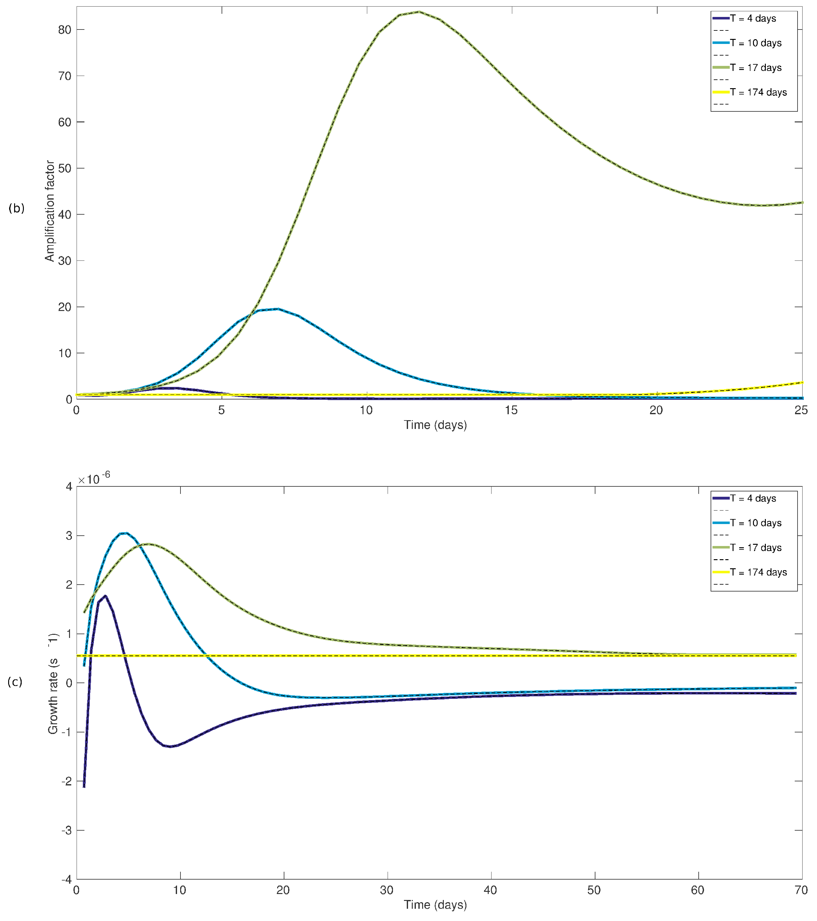
Figure 10.
Time evolution of the optimal perturbation for a time interval = 17 days in the non-linear QG model. The colour scale shows the PVA perturbation () while the black contours show the total PVA q. The top panels show horizontal sections of PVA through the vortex core, the middle panels show horizontal sections of PVA through the vortex lobes and the bottom panels show vertical sections of PVA.
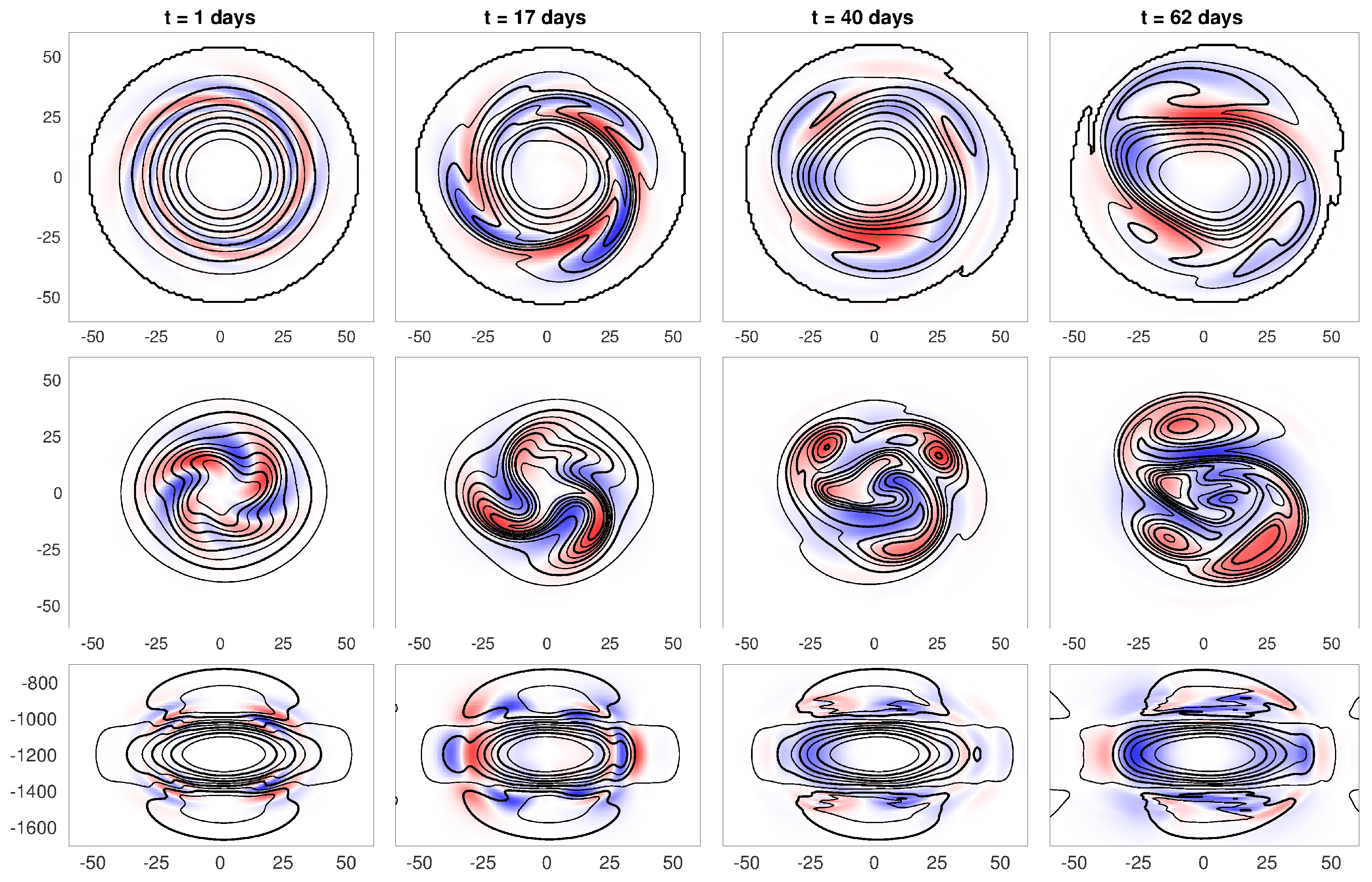
Figure 11.
Time evolution of the azimuthal decomposition of the optimal perturbation for a time interval = 17 days integrated in the non-linear QG model. The discontinuous black line shows the total energy.
Figure 11.
Time evolution of the azimuthal decomposition of the optimal perturbation for a time interval = 17 days integrated in the non-linear QG model. The discontinuous black line shows the total energy.
© 2018 by the authors. Licensee MDPI, Basel, Switzerland. This article is an open access article distributed under the terms and conditions of the Creative Commons Attribution (CC BY) license (http://creativecommons.org/licenses/by/4.0/).
Share and Cite
MDPI and ACS Style
Meunier, T.; Ménesguen, C.; Carton, X.; Le Gentil, S.; Schopp, R. Optimal Perturbations of an Oceanic Vortex Lens. Fluids 2018, 3, 63. https://doi.org/10.3390/fluids3030063
AMA Style
Meunier T, Ménesguen C, Carton X, Le Gentil S, Schopp R. Optimal Perturbations of an Oceanic Vortex Lens. Fluids. 2018; 3(3):63. https://doi.org/10.3390/fluids3030063
Chicago/Turabian StyleMeunier, Thomas, Claire Ménesguen, Xavier Carton, Sylvie Le Gentil, and Richard Schopp. 2018. "Optimal Perturbations of an Oceanic Vortex Lens" Fluids 3, no. 3: 63. https://doi.org/10.3390/fluids3030063