Onset of Convection in the Presence of a Precipitation Reaction in a Porous Medium: A Comparison of Linear Stability and Numerical Approaches

1
Department of Chemical Engineering and Biotechnology, University of Cambridge, Cambridge CB3 0AS, UK
2
Department of Chemical Engineering, Jadavpur University, Kolkata 700032, India
3
Department of Chemical Engineering, Jeju National University, Jeju 63243, Korea
*
Author to whom correspondence should be addressed.
Fluids 2018, 3(1), 1; https://doi.org/10.3390/fluids3010001
Submission received: 2 November 2017
/
Revised: 8 December 2017
/
Accepted: 17 December 2017
/
Published: 22 December 2017
(This article belongs to the Special Issue Convective Instability in Porous Media)
Abstract
:Reactive convection in a porous medium has received recent interest in the context of the geological storage of carbon dioxide in saline formations. We study theoretically and numerically the gravitational instability of a diffusive boundary layer in the presence of a first-order precipitation reaction. We compare the predictions from normal mode, linear stability analysis, and nonlinear numerical simulations, and discuss the relative deviations. The application of our findings to the storage of carbon dioxide in a siliciclastic aquifer shows that while the reactive-diffusive layer can become unstable within a timescale of 1 to 1.5 months after the injection of carbon dioxide, it can take almost 10 months for sufficiently vigorous convection to produce a considerable increase in the dissolution flux of carbon dioxide.
1. Introduction
Motivated by the processes occurring during the geological storage of carbon dioxide in saline aquifers, we theoretically investigated the gravitational instability of a diffusive boundary layer in a porous medium in the presence of a precipitating chemical reaction. In the geological storage of carbon dioxide in saline aquifers (800–1000 m below the Earth’s surface), carbon dioxide dissolves in brine and drives dissolution-driven natural convection, which in turn can drive further convection and thereby accelerate the storage procedure. Accelerated dissolution reduces the possibilities of upward flow of free-phase CO2, potentially leaking through any high permeability zones or artificial penetrations, such as abandoned wells [1]. Convection brings carbon dioxide-rich fluid downward and fresh fluid upward, effectively enhancing the transport of carbon dioxide into the saline aquifer. It was widely believed that these convection streams transport the dissolved and entrapped carbon dioxide in brine efficiently to depth. Recent studies, however, have questioned this very basic assumption. Preliminary results [2,3,4,5] strongly indicated that geochemical reactions between dissolved carbon dioxide and the subsurface rock matrix may have a non-negligible effect on the convective mixing in the boundary layer.
In this paper, we compare the results of a linear stability analysis using three different methods, namely the dominant mode of a self-similar diffusion operator [6], an initial-value-problem approach [7], and a quasi-steady state assumption (QSSA) method [8] for a reactive-diffusive boundary layer in a porous medium where the product of a first-order reaction precipitates out from the system (Figure 1). We also compare the time for onset of convection from these linear stability methods with that obtained from nonlinear numerical simulations [3]. The results from the dominant mode analysis are new, while the results from the other methods were obtained from previous literature. Finally, we discuss the implications of our results in the context of the geological storage of carbon dioxide in a siliciclastic aquifer.
2. Model
We present the governing equations and the scaling for a reactive-diffusive boundary layer in a porous medium, along with the linear stability equations, in this section. The solution methodologies of the stability equations are also discussed.
2.1. Governing Equations and Scaling
The transport of a solute is considered as it dissolves at the top of a fluid-saturated porous medium. A two-dimensional, homogeneous, isotropic porous medium is considered (Figure 1). The solute dissolves in the underlying fluid, forming a diffusive boundary layer of higher density than the underlying fluid. The solute remains unstably distributed in the fluid, causing gravitational instability of the diffusive layer as it deepens. We consider the chemical reaction between the solute with chemical species present in the host porous rock, resulting in an insoluble product The product , being precipitated out, does not contribute to the density of the solution. As species is in the solid phase, we assume its concentration to be constant, so that the reaction rate depends only the concentration of species and is taken to be first-order. The continuity equation for the incompressible fluid, Darcy’s law with the Boussinesq assumption, and the conservation equation of the dissolved species are then given by:
here, is the Darcy velocity vector, is the viscosity of the fluid, is the reduced pressure field, obtained by eliminating hydrostatic pressure from the local pressure , is the acceleration due to gravity, is a vertical unit vector co-directional with the positive axis, and is time. The isotropic permeability and the porosity of the porous medium are assumed to remain unchanged by the chemical reaction. The local concentration of the diffusing solute is . The local density of the fluid is assumed to be linearly dependent on the local concentration of the solute: ; the reference density is that of the pure fluid and the solutal expansion coefficient is defined as . The reaction rate per unit concentration of fluid is , and is assumed to be constant; here, the solid based kinetic rate constant is and the reactive surface area per mole of the solid is . The effective diffusivity of the dissolved species in the porous medium is taken as the product of the molecular diffusion coefficient and the porosity of the aquifer since only the fluid-saturated void region of the porous medium participates in the diffusive mass transfer. Tortuosity of the porous medium is assumed to be small and convective dispersion is neglected with respect to the molecular diffusion.
The above equations are non-dimensionalized using the scales , ,,, and the solubility concentration of solute in the fluid , giving [3]:
here, is Damköhler number and is the solutal Rayleigh number; is the vertical lengthscale of the reservoir. The Damköhler number is a measure of the ratio of the diffusive timescale to the reactive timescale. The solutal Rayleigh number signifies the ratio of the driving buoyancy force for convection to the viscous and diffusive dissipation, which inhibits convection [9]. The maximum density contrast between the pure and solute-saturated fluid is . The dynamics of such a reactive boundary layer is therefore fully determined by only one dimensionless group, , which measures the timescale for convection compared to those for reaction and diffusion. The internal length scale is a measure of the thickness of the boundary layer at instability.
The porous medium is considered to be infinite in the horizontal direction and semi-infinite in the vertical direction (, taken as a positive downward). This simplification is valid while the penetration depth is smaller than the domain depth, i.e., for a short time period. At time , the entire domain is quiescent and solute-free, i.e., and . The top boundary has the maximum concentration of solute and is impermeable to the fluid, and , at the bottom boundary.
2.2. Linear Stability Analysis
The concentration, velocity components, and pressure are decomposed into non-convective base state and perturbation components such that:
here, subscript ‘b’ denotes the base state and caret denotes the perturbation components. The base state velocity components are zero and the base state concentration profile is [5]:
The perturbation equations are linearized and the horizontal and the vertical components of the momentum balance equation are cross-differentiated and added to eliminate pressure. The resulting equations are again differentiated and rearranged to eliminate horizontal velocity component, resulting in the following equations involving the perturbation concentration and perturbation velocity in the vertical direction:
All variables are in dimensionless form and the superscript “″ is dropped for simplicity. The solutions of Equations (9) and (10) are decomposed into normal modes in the horizontal direction with wave number as:
Using Equation (11) in Equations (9) and (10), we obtain:
with the boundary conditions for and for
After coordinate transformation Equations (12) and (13) become:
with boundary conditions for and for The above transformation enables us to obtain a self similar diffusion operator in the streamwise direction and leads to eigen functions which are localized around the base concentration profile. Riaz et al. [10] and Rees et al. [11] used this approach for an inert system and obtained considerable improvement in the accuracy of the solutions. Here, we use a similar approach for a reactive system with a precipitating product.
The streamwise operator of the perturbation concentration in the transformed coordinate is:
The perturbation concentration is expanded as:
with
The eigen functions are Hermite polynomials, in a semi-infinite domain with weight functions with the associated eigen values for [10]. These eigen functions are localized around the base state.
Considering Equations (14) and (15) in the limit of zero wave number, and using Expression (17), it can be shown that the first mode, , decays at the slowest rate, compared to the other modes, and is therefore considered the dominant mode, following Riaz et al. [10]. Considering only the dominant mode, the perturbation concentration becomes:
where is a function of time. We use the dominant mode approximation for (11) in Equation (15) to obtain:
We integrate Equation (19) in the space domain and define the growth rate of perturbation concentration as:
following Riaz et al. [10]. Expression (18) is used in Equation (14) and an analytical solution for the velocity is obtained:
The growth rate of perturbation in Equation (20) was obtained semi-analytically. Suffix ‘p’ in denotes precipitating reaction. Also, suffix ‘1’ in denotes the dominant mode.
In the initial-value problem approach [7], Equations (14) and (15) were solved using the finite-element method in partial-differential equation solver Fastflo [12]. Test simulations were conducted to ensure that the results became independent of particular initial conditions well below the times for onset of instability, and agreed with previously published solutions for the inert system. The concentration perturbation was measured using the norm:
where is the extent of the computational domain. Although this norm depends on the domain length scale , we only use it to measure the non-dimensional growth rate of this perturbation, defined as:
Beside the above dominant mode method and the initial value problem approach, we solved the above stability equations using the quasi-steady state assumption (QSSA). Under the QSSA, we assume that the perturbations and can be expressed as:
Then, Equation (15) can be rephrased as:
In the present study, we solved the eigenvalue problem of Equations (14) and (25) using the outward shooting method explained by Kim and Choi [13,14]. Kim and Choi [14] showed that for the non-reactive case, i.e., , the present QSSA represents the exact solution quite well. We note there are many methods to solve numerical eigenvalue problems. Other researchers used spectral methods such as Chebyshev tau and Chebyshev collocation methods rather than the present method. However, as far as we know, the results are independent of the solution method.
3. Results
In this section we discuss the effect of a first-order precipitation reaction on the growth rate of perturbations considering the dominant mode of a self-similar diffusion operator. We then compare the neutral stability criteria, the time for onset of convection, and the most unstable wave number at the onset of instability compared to those obtained previously using different methods of analysis.
3.1. Growth Rate of the Perturbation
The growth rates of the perturbations are investigated as a function of time (t) and wave numbers (k) for an inert, weak reaction and a strong reaction, as shown in Figure 2 and Figure 3. For the inert system (), at small times the growth rate is negative for all wave numbers, suggesting that the layer is unconditionally stable for all possible disturbance modes. As time progresses, the growth rate increases and eventually becomes positive when a sufficient amount of heavy solute has accumulated in the layer and overcomes the stabilizing effect of viscosity, resulting in gravitational instability. Following this, the layer continues to remain unstable. The growth rate is also dependent on the perturbation modes, measured by wave numbers, and there are small and large wave number cut-offs beyond which the layer remains stable. Below the small wave number cut-off, the accumulated dense material is insufficient to drive convection. Above the large wave number cut-off, horizontal diffusion stabilizes the system. In the presence of a weak reaction, , the nature of the plot remains similar; however, the growth rate significantly decreases, confirming a stabilization effect in the presence of a chemical reaction (Figure 3a). Chemical reaction enhances the stability by removing the solute in the form of an insoluble product, which would otherwise dissolve in the fluid and increase the density contrast, resulting in instability. The precipitating reaction causes an increase in the time for onset of instability and a decrease in the range of unstable wave numbers, as elaborated in the subsequent sections. For higher reaction strength (), the growth rate becomes even smaller and remains positive for only a very short period of time (Figure 3b), suggesting the termination of convection after a certain time. Above of the growth rate remains negative for all possible disturbance modes, the layer becomes stable and mass transfer occurs only through diffusion and chemical reaction, as discussed in the subsequent sections. The growth rates of the perturbations as a function of wave numbers for are shown in the two-dimensional plots at non-dimensional time in Figure 4.
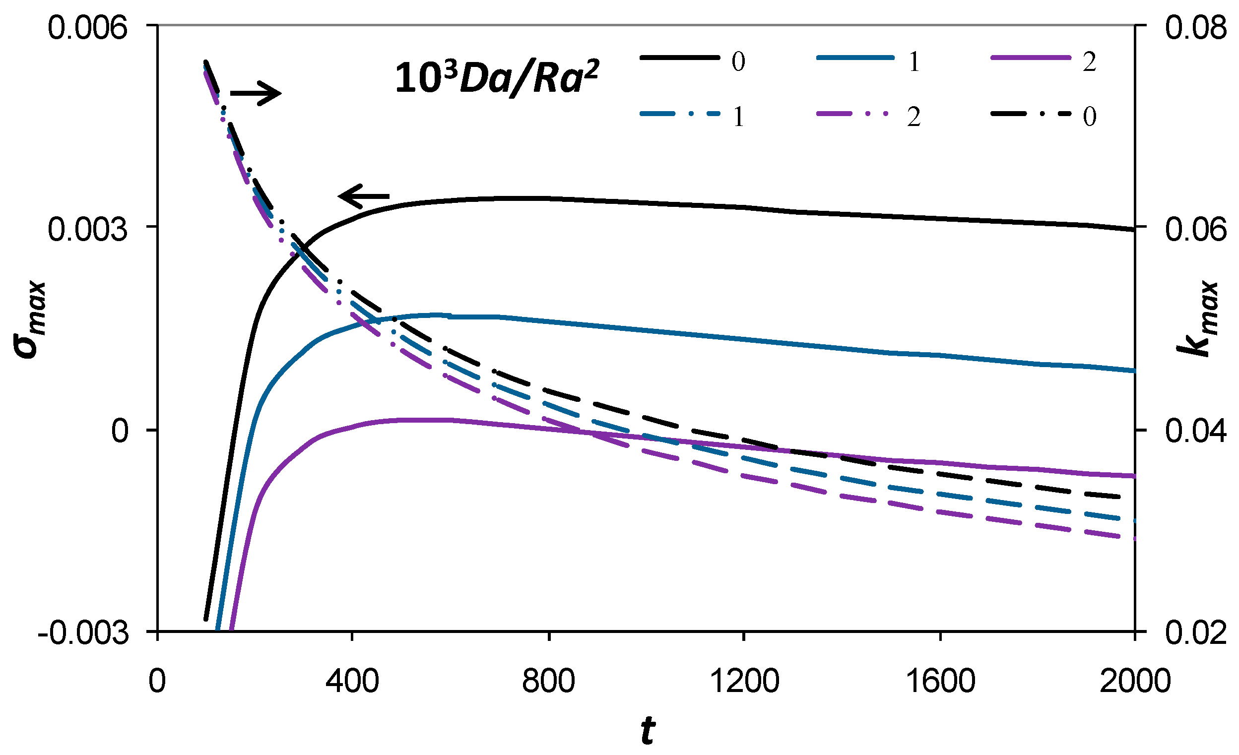
3.2. Maximum Growth Rate and Corresponding Wave Number
Since the growth rate is a function of the wave number (or horizontal perturbation mode) at each time point, it is necessary to obtain the maximum growth rate at each time point and the corresponding wave number. The maximum growth rate and the corresponding most dangerous wave number was investigated as a function of time for three different values of Da/Ra2, as shown in Figure 5. The maximum growth rate increases rapidly at early times, as the solute diffuses and accumulates in the layer, and decreases slowly over a long period of time. As Da/Ra2 increases, the maximum growth rate decreases, as the density of the layer decreases owing to the removal of the solute in the form of a precipitating product from the system. The most dangerous wave number decreases from 0.075 to 0.03 as time varies between 100 and 2000. The most dangerous wave number is weakly dependent on Da/Ra2, decreasing slightly for higher Da/Ra2.
3.3. Marginal Stability Curves
The effects of a precipitating reaction on the marginal stability curves are investigated in Figure 6, using an initial value problem approach, the dominant mode analysis, and a quasi-steady state assumption. Each U-shaped curve indicates the neutral state when the boundary layer is marginally stable and the growth rate of perturbation becomes zero. The time for onset of instability is a function of the horizontal perturbation mode (wave number) for a given . The black solid line represents an inert system (). Below this line, the growth rates of perturbations are negative and the system remains stable. Above this line, the growth rates are positive and the layer is gravitationally unstable. As increases ( in Figure 6b), the curves shift upward, indicating a delay in the onset of instability. The region of instability also shrinks from both sides, signifying a reduction in the range of unstable wave numbers. As the reaction strength increases further (), the curves close at the top, suggesting a brief period of convection beyond which motion ceases and the layer again stabilizes. Thus, for sufficiently large Da/Ra2, convection develops over a finite period of time only. A further increase in reaction strength leads to significant shrinkage of the unstable zone. Above a critical value of 103 Da/Ra2 ~ 2.1, using a dominant mode analysis, the reaction stabilizes the system completely.
The marginal stability curves obtained using the initial value problem approach, the dominant mode analysis, and the quasi-steady state assumption differ quantitatively, as shown in Figure 6a–c. Figure 7 focuses on the comparison for . Among the three methods of analysis, the initial value problem approach predicts the lower bound for the critical time of instability and the upper bound for the large wave number cut-off for the inert, moderate, and strong reactive cases. The small wave number cut-off was found to be fairly insensitive to the method employed, for inert and moderately strong reactions. At high reaction strength, the finite domain of instability, as indicated by the closed curves, was found to vary with the method used: the initial value approach predicts the shortest period of convection while the quasi-steady state assumption predicts the longest.
3.4. Time for Onset of Convection
The impact of a precipitating reaction on the time for onset of instability predicted using the different methods is shown in Figure 8. The critical time for onset of instability corresponds to the time at which the maximum growth rate of perturbation, with respect to all wave numbers, becomes positive. This is the minimum time for onset of instability under all possible disturbance modes. It is evident in the figure that all the methods predict that as increases, the critical time for onset of instability increases as the layer stabilizes owing to the removal of the solute in the form of an insoluble product. For rapid chemical reaction, the dotted line indicates the time at which convection ceases following temporary convection. As mentioned in the previous section, beyond a critical value ( from dominant mode analysis, using initial value problem approach), convection does not occur as the reaction stabilizes the diffusive layer. The time for onset of convection from the nonlinear numerical simulation, the time at which the dissolution flux transitions from diffusive to the convective regime [3], is substantially higher than the time for onset of instability obtained from the linear stability analysis.
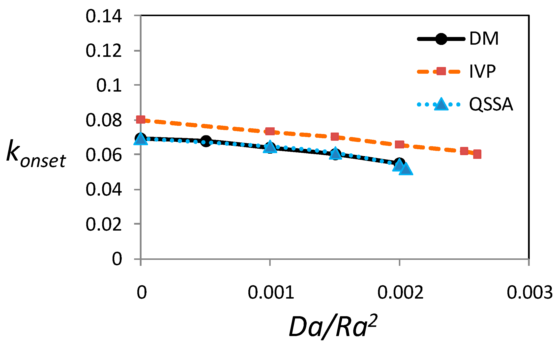
3.5. Critical Wave Number at the Onset of Instability
The effect of a precipitating reaction on the most unstable wave number at the onset of instability was investigated using the dominant mode analysis, initial value problem approach, and the quasi-steady state assumption (Figure 9). The most unstable wave number at the onset of instability slowly decreases with for all three methods. This gradual reduction in wave number arises from the increase in the time for onset of instability with reaction strength and a decrease in most unstable wave number with time. The reduction in the most unstable wave number as time progresses originates from a weakening of the stabilization by vertical diffusion compared to that by transverse diffusion. It is evident from the plot that the critical wave number at the onset of instability predicted by the dominant mode analysis and using the quasi-steady state assumption are in excellent agreement for all reaction strengths. The initial value problem approach predicts a slightly larger wave number. For an inert system, the most unstable wave number at the onset of instability is in agreement with previously published results [10,11], thus validating our methodology.
4. Discussion and Conclusions
In the recent past, various methods [3,5,7,8,15] have been employed to investigate the stability of a diffusive layer undergoing a first-order precipitating reaction in a porous medium. In this paper we examine the linear stability of such a diffusive layer using the dominant mode of a self-similar diffusion operator [6] and compare the marginal stability curves, the time for onset of convection, and the most critical wave number at the onset of instability to those previously predicted using different methods.
The linear stability analysis using the dominant mode of the self-similar diffusion operator and considering a quasi-steady state approximation have previously been applied for dissolution-driven convection in inert systems [10,11]. One important characteristic of the dissolution-driven convection problem is the time-varying concentration base profile. The dominant mode solution is advantageous in this case since it does not require the quasi-steady state approximation. The dominant mode solution has been found to accurately predict the instability of the diffusive layer for inert systems [10]. However, for an inert system the dominant mode solution has been reported to be less accurate for longer periods of time and solutions based on the quasi-steady state approximation have been suggested. These two methods are therefore mutually complementary since the quasi-steady condition is applicable to long time periods when the base state concentration changes slowly. We therefore compare the results using these two methods for the situation where the dissolved solute undergoes a precipitating reaction and alters the base state concentration profile and thereby the density field. Our comparison suggests that for a reactive system, the critical wave numbers at the onset of instability predicted using these methods are in good agreement.
At low and moderate reaction strengths, the time for onset of convection predicted by the dominant mode analysis and the initial-value problem approach are in reasonable agreement. The deviations between the results are comparable with those observed for the inert system. The deviations in the marginal stability curves obtained using the three methods are also in agreement, with discrepancies observed for the inert system. The difference between the results from the dominant mode analysis and the initial value problem approach arises from the fact that the initial-value problem approach is the full solution of the linear stability equation, while the dominant mode analysis considers only the dominant mode of the self-similar diffusion operator. In contrast to the complete nonlinear simulations, linear stability solutions are valid for short time periods and small perturbations since the linearized equations are considered.
The general variation of the onset time with reaction strength predicted from nonlinear numerical simulations is in agreement with that obtained from the linear stability analysis. For inert systems, Hassanzadeh et al. [1] reported the time for onset of convection from numerical simulation to be almost an order of magnitude higher than that obtained from linear stability analysis. For the reactive system studied here, the ratio of time for onset of convection obtained from nonlinear simulations, to that from linear stability, is of this order and is therefore acceptable. The reason for this discrepancy between the linear and non-linear results has been explained by previous researchers for inert systems. For inert systems, it was shown that following the onset of motion, the Fickian diffusion continues to dominate for a substantial period of time, with convective fingers being almost imperceptible until the perturbations are considerably large to cause a significant increase in the rate of solute dissolution at the top interface [16,17]. This time corresponds to the onset time of non-linear instability [18]. Here, we confirm a similar behavior in the reactive system.
The above variations in the time for onset of reactive convection can have substantial implications in the geological storage of carbon dioxide in saline aquifers, where the carbon dioxide dissolved in brine reacts with the porous rock matrix. An important example of this type of reaction is a precipitation reaction between carbon dioxide-rich brine and a rock formation rich in calcium feldspar; here, the dissolved carbon dioxide is removed from solution in precipitate products calcite and kaolinite [7,19]. Considering typical reservoir permeability, m2, and porosity, , we estimate that . In this situation, considering , we predict the time for onset of instability to be 1.5 month and 1 month using the dominant mode analysis and initial value problem analysis, respectively. The time for onset of convection based on nonlinear simulation is estimated to be10 months. This means that although the reactive-diffusive layer becomes unstable ~1–1.5 months after the injection of carbon dioxide into the saline formation, substantial convective motion starts only ~10 months after injection. Only at this time does the dissolution flux of carbon dioxide into the brine increase significantly.
As a final remark, we note that the present study focused on a two-dimensional spatial model. This is certainly a good starting system given that two-dimensional flow in a porous medium is easily investigated in the laboratory with a Hele-Shaw cell. The modeling results can therefore be compared and validated with laboratory measurements. Of course, it would be interesting to explore a three-dimensional spatial system in the future.
Acknowledgments
Parama Ghoshal gratefully acknowledges Manmohan Singh Scholarship from St. John’s College, Cambridge, U.K. and the grant of study leave from Jadavpur University, Kolkata, India.
Author Contributions
Parama Ghoshal, Min Chan Kim and Silvana S. S. Cardoso conceived and designed the study; Parama Ghoshal performed the Dominant-Mode analysis; Silvana S. S. Cardoso performed the Initial-Value-Problem analysis; Min Chan Kim performed the Quasi-Steady-State analysis. All authors contributed to the writing of the paper.
Conflicts of Interest
The authors declare no conflict of interest.
References
- Hassanzadeh, H.; Pooladi-Darvish, M.; Keith, D.W. Scaling behavior of convective mixing, with application to geological storage of CO2. AIChE J. 2007, 53, 1121–1131. [Google Scholar] [CrossRef]
- Ennis-King, J.; Paterson, L. Coupling of geochemical reactions and convective mixing in the long-term geological storage of carbon dioxide. Int. J. Greenh. Gas Control 2007, 1, 86–93. [Google Scholar] [CrossRef]
- Andres, J.T.H.; Cardoso, S.S. Onset of convection in a porous medium in the presence of chemical reaction. Phys. Rev. E 2011, 83, 046312. [Google Scholar] [CrossRef] [PubMed]
- Ghesmat, K.; Hassanzadeh, H.; Abedi, J. The impact of geochemistry on convective mixing in a gravitationally unstable diffusive boundary layer in porous media: CO2 storage in saline aquifers. J. Fluid Mech. 2011, 673, 480–512. [Google Scholar] [CrossRef]
- Andres, J.T.H.; Cardoso, S.S. Convection and reaction in a diffusive boundary layer in a porous medium: Nonlinear dynamics. Chaos 2012, 22, 037113. [Google Scholar] [CrossRef] [PubMed]
- Ghoshal, P. Studies on Dissolution-Driven Convection with Precipitating and Non-Precipitating Chemical Reactions in Porous Media. Ph.D. Thesis, University of Cambridge, Cambridge, UK, 2016. [Google Scholar]
- Cardoso, S.S.S.; Andres, J.T.H. Geochemistry of silicate-rich rocks can curtail spreading of carbon dioxide in subsurface aquifers. Nat. Commun. 2014, 5, 5743. [Google Scholar] [CrossRef] [PubMed]
- Kim, M.C.; Kim, Y.H. The effect of chemical reaction on the onset of gravitational instabilities in a fluid saturated within a vertical Hele-Shaw cell: Theoretical and numerical studies. Chem. Eng. Sci. 2015, 134, 632–647. [Google Scholar]
- Linden, P.F. Perspectives in Fluid Dynamics, Chapter 6: Convection in the Environment; Batchelor, G.K., Moffatt, H.K., Worster, M.G., Eds.; Cambridge University Press: Cambridge, UK, 2000. [Google Scholar]
- Riaz, A.; Hesse, M.; Tchelepi, H.A.; Orr, F.M. Onset of convection in a gravitationally unstable diffusive boundary layer in porous media. J. Fluid Mech. 2006, 548, 87–111. [Google Scholar] [CrossRef]
- Rees, D.A.S.; Selim, A.; Ennis-King, J.P. The instability of unsteady boundary layers in porous media. In Emerging Topics in Heat and Mass Transfer in Porous Media; Springer: Dordrecht, The Netherlands, 2008; pp. 85–110. [Google Scholar]
- Commonwealth Scientific and Industrial Research Organisation (CSIRO). Fastflo Tutorial Guide; CSIRO: Canberra, Australia, 2000. [Google Scholar]
- Kim, M.C.; Choi, C.K. Effects of first-order chemical reaction on gravitational instability in a porous medium. Phys. Rev. E 2014, 90, 053016. [Google Scholar] [CrossRef] [PubMed]
- Kim, M.C.; Choi, C.K. Some theoretical aspects on the onset of buoyancy-driven convection in a fluid-saturated porous medium heated impulsively from below. Korean J. Chem. Eng. 2015, 32, 2400–2405. [Google Scholar] [CrossRef]
- Ward, T.J.; Cliffe, K.A.; Jensen, O.E.; Power, H. Dissolution-driven porous medium convection in the presence of chemical reaction. J. Fluid Mech. 2014, 747, 316–349. [Google Scholar] [CrossRef]
- Slim, A.C. Solutal-convection regimes in a two-dimensional porous medium. J. Fluid Mech. 2014, 741, 461–491. [Google Scholar] [CrossRef]
- Emami-Meybodi, H.; Hassanzadeh, H.; Green, C.P.; Ennis-King, J. Convective dissolution of CO2 in saline aquifers: Progress in modeling and experiments. Int. J. Greenh. Gas Control 2015, 40, 238–266. [Google Scholar] [CrossRef]
- Tilton, N.; Daniel, D.; Riaz, A. The initial transient period of gravitationally unstable diffusive boundary layers developing in porous media. Phys. Fluids 2013, 25, 092107. [Google Scholar] [CrossRef]
- Marini, L. Geological Sequestration of Carbon Dioxide: Thermodynamics, Kinetics, and Reaction Path Modeling; Elsevier: Amsterdam, The Netherlands, 2007; Volume 11. [Google Scholar]
Figure 1.
Solute dissolves in the underlying fluid, forming a diffusive boundary layer. Dissolution enhances the local density difference between the solute-saturated fluid at the interface and the underlying pure fluid, driving finger formation and convection. Dissolved solute A reacts with reactant species in the host rock, forming product , which precipitates out from the fluid. Chemical reaction alters the spatial distribution of the solute and thereby changes the density field.
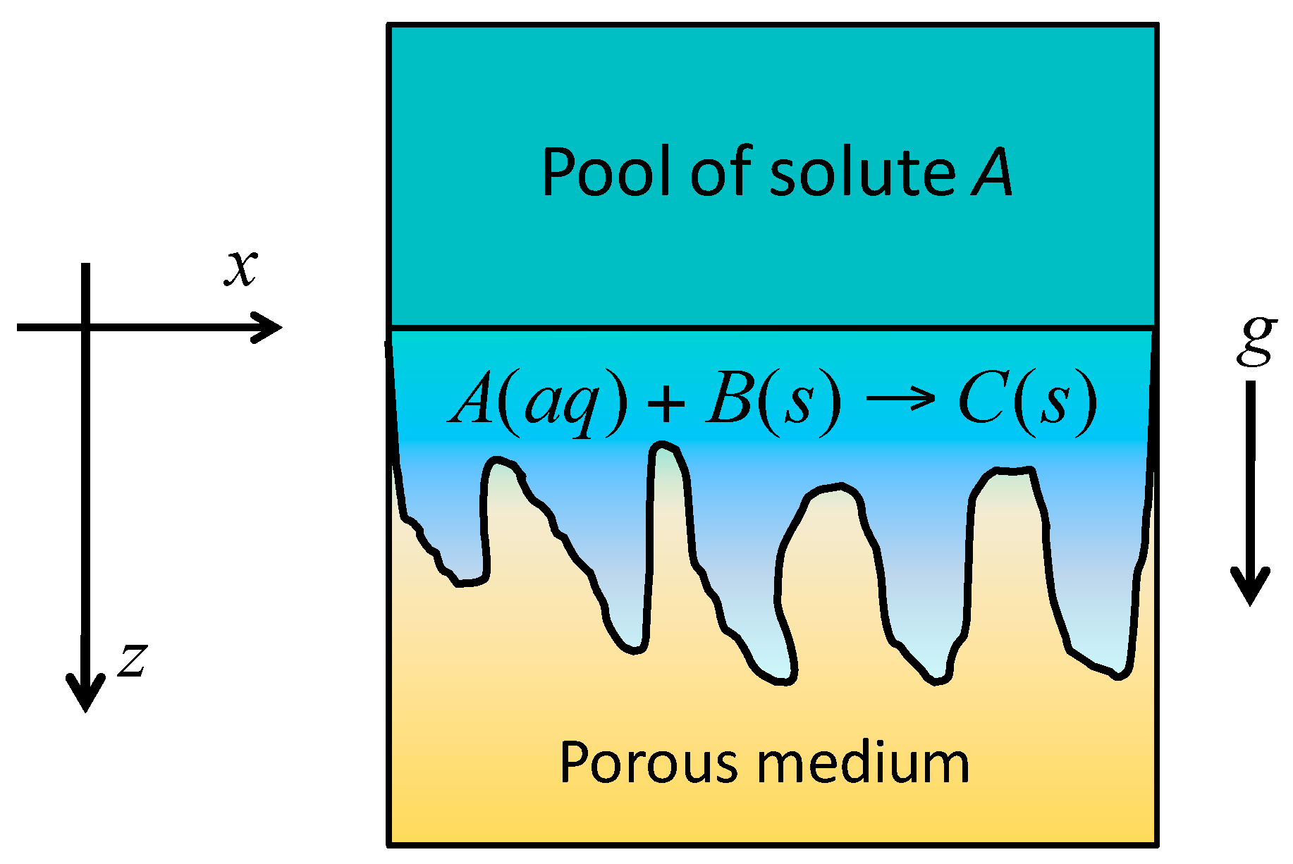
Figure 2.
Variation of the growth rate of perturbations with wave number and time for the inert system using the dominant mode analysis.
Figure 2.
Variation of the growth rate of perturbations with wave number and time for the inert system using the dominant mode analysis.

Figure 3.
Variation of the growth rate of perturbations with wave number and time for a reactive system: (a) weak reaction (); (b) strong reaction (), using the dominant mode analysis.
Figure 3.
Variation of the growth rate of perturbations with wave number and time for a reactive system: (a) weak reaction (); (b) strong reaction (), using the dominant mode analysis.
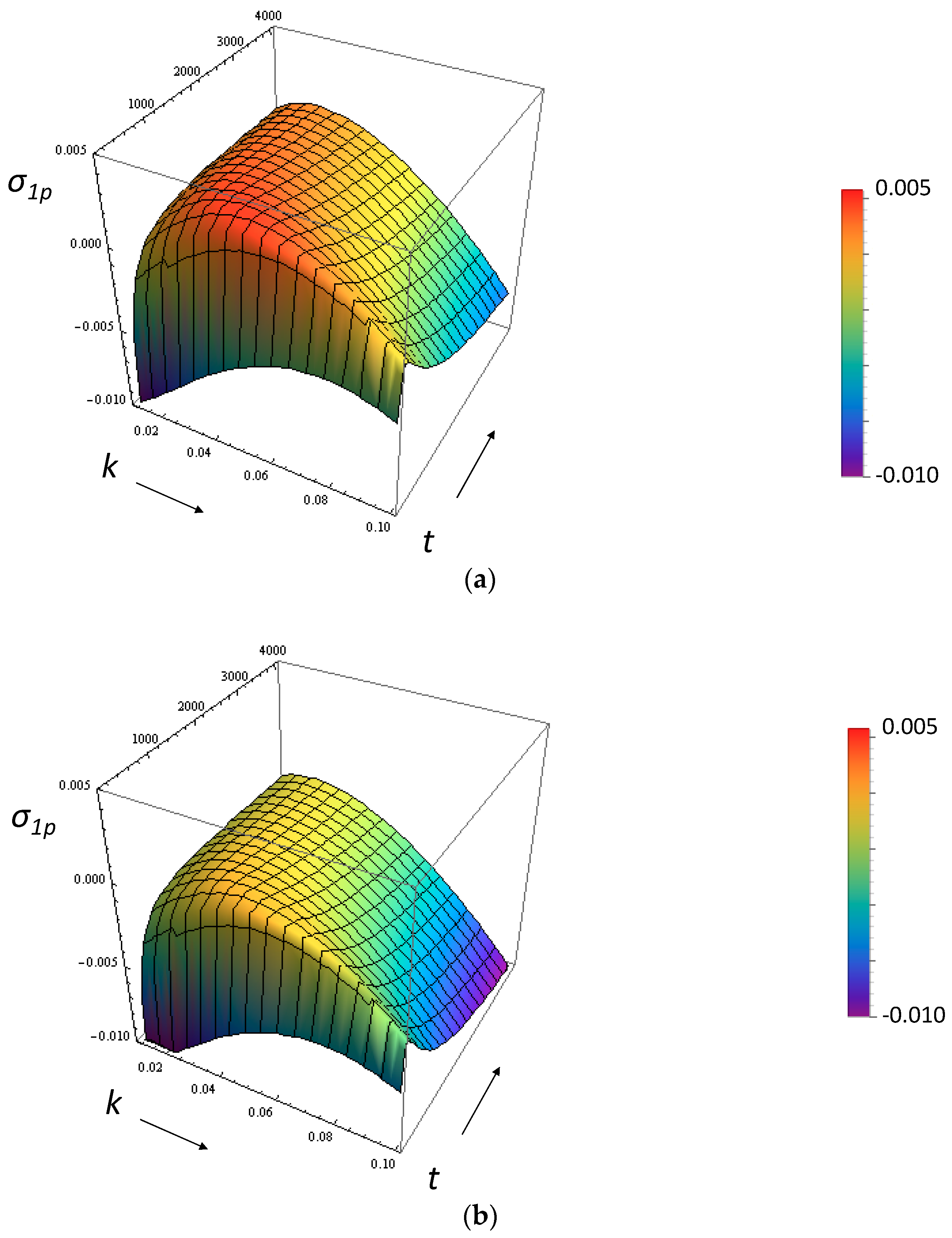
Figure 4.
Growth rate of perturbations as a function of wave number for different at non-dimensional .
Figure 4.
Growth rate of perturbations as a function of wave number for different at non-dimensional .
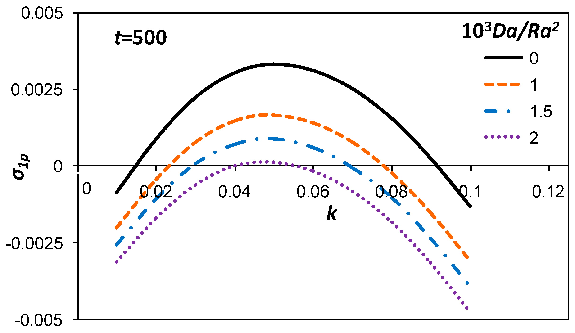
Figure 5.
The maximum growth rate of perturbations and the corresponding most unstable wave number as a function of time, for three different , using the dominant mode analysis.
Figure 5.
The maximum growth rate of perturbations and the corresponding most unstable wave number as a function of time, for three different , using the dominant mode analysis.

Figure 6.
Effect of a precipitating reaction on the marginal stability boundary using (a) an initial-value problem approach [7]; (b) the dominant mode analysis; and (c) the quasi-steady state assumption (QSSA) method.
Figure 6.
Effect of a precipitating reaction on the marginal stability boundary using (a) an initial-value problem approach [7]; (b) the dominant mode analysis; and (c) the quasi-steady state assumption (QSSA) method.
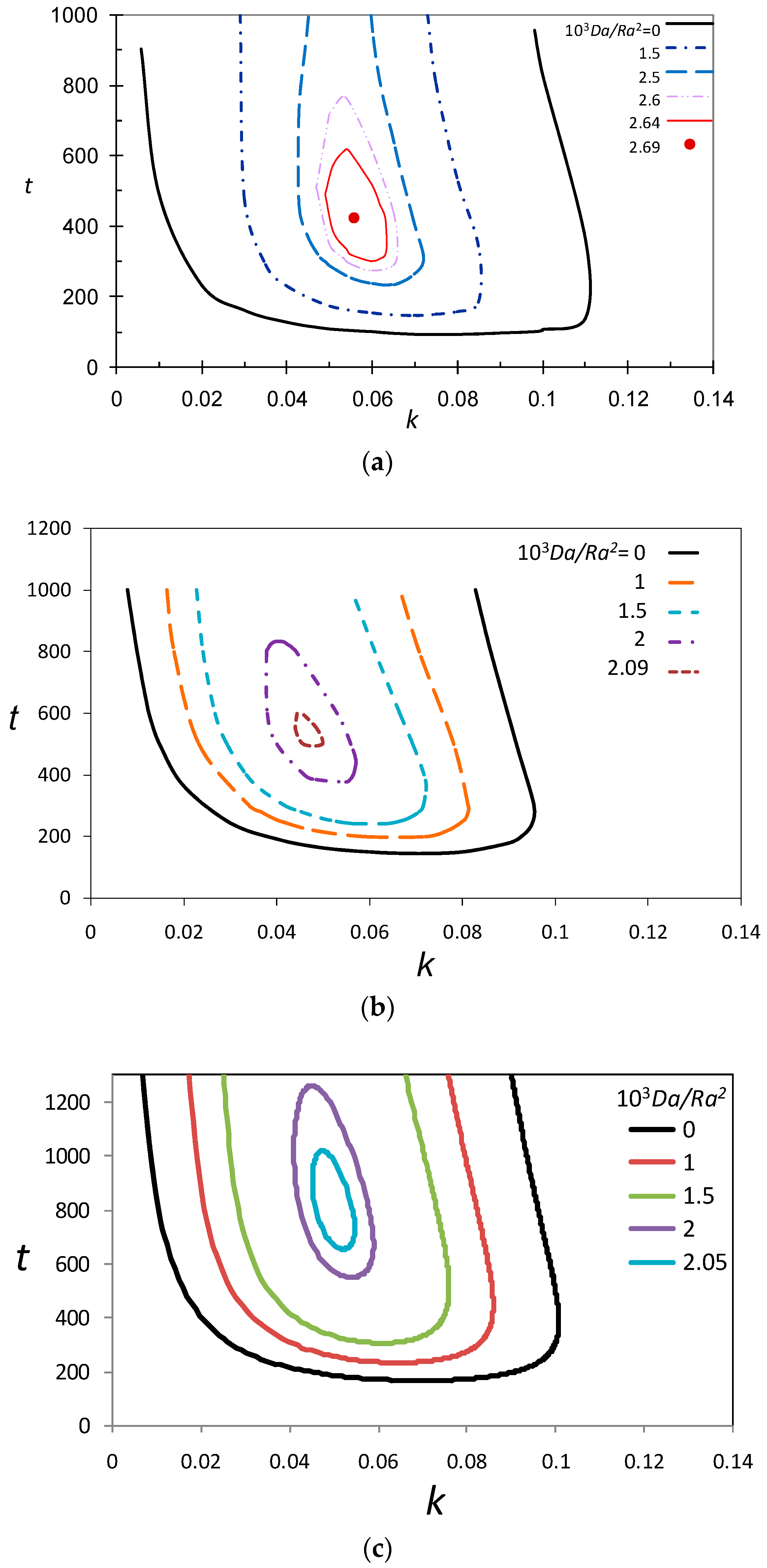
Figure 7.
Comparison of neutral stability curves obtained using an initial-value problem approach (IVP), the dominant mode analysis (DM), and the quasi-steady state assumption (QSSA) method for (a) ; (b) ; and (c) .
Figure 7.
Comparison of neutral stability curves obtained using an initial-value problem approach (IVP), the dominant mode analysis (DM), and the quasi-steady state assumption (QSSA) method for (a) ; (b) ; and (c) .
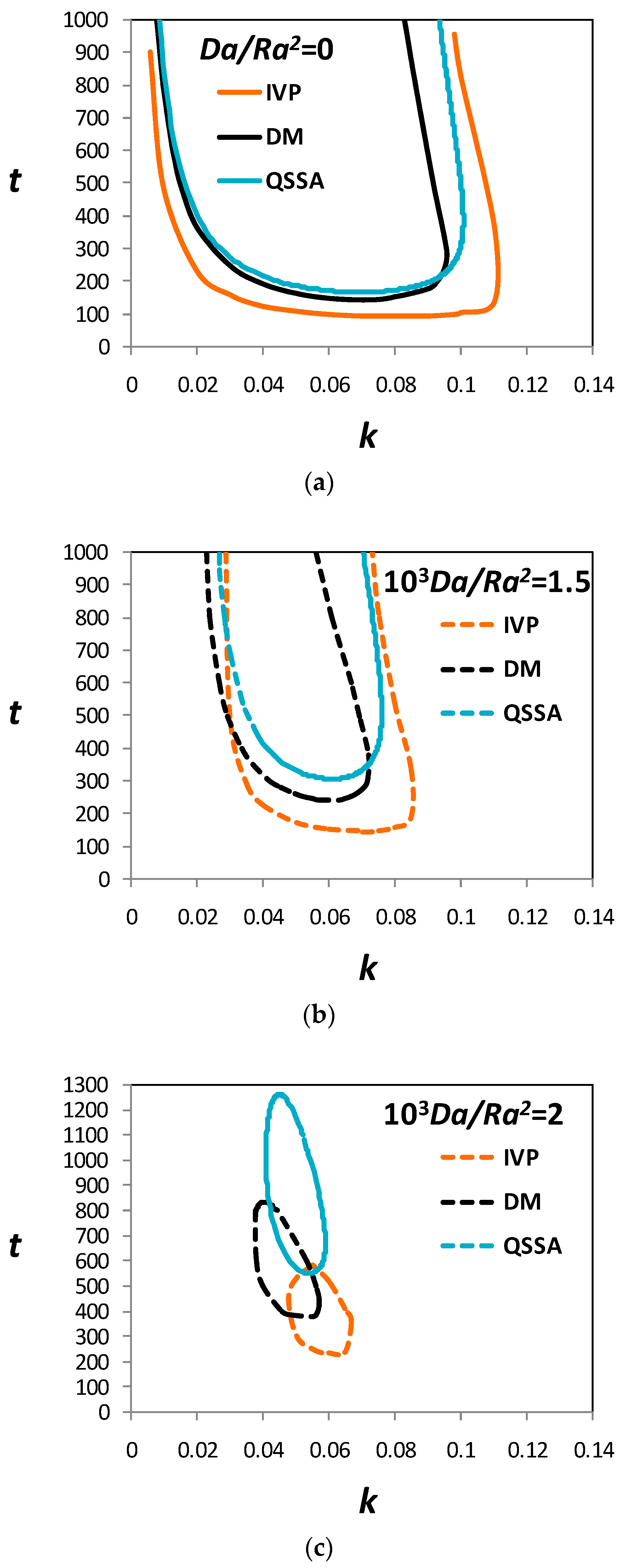
Figure 8.
Non-dimensional time for onset and cessation of convection (dimensionless) as a function of for a precipitating reaction, predicted using the dominant mode analysis (DM), initial-value problem approach (IVP), and nonlinear numerical simulations (NNS).
Figure 8.
Non-dimensional time for onset and cessation of convection (dimensionless) as a function of for a precipitating reaction, predicted using the dominant mode analysis (DM), initial-value problem approach (IVP), and nonlinear numerical simulations (NNS).
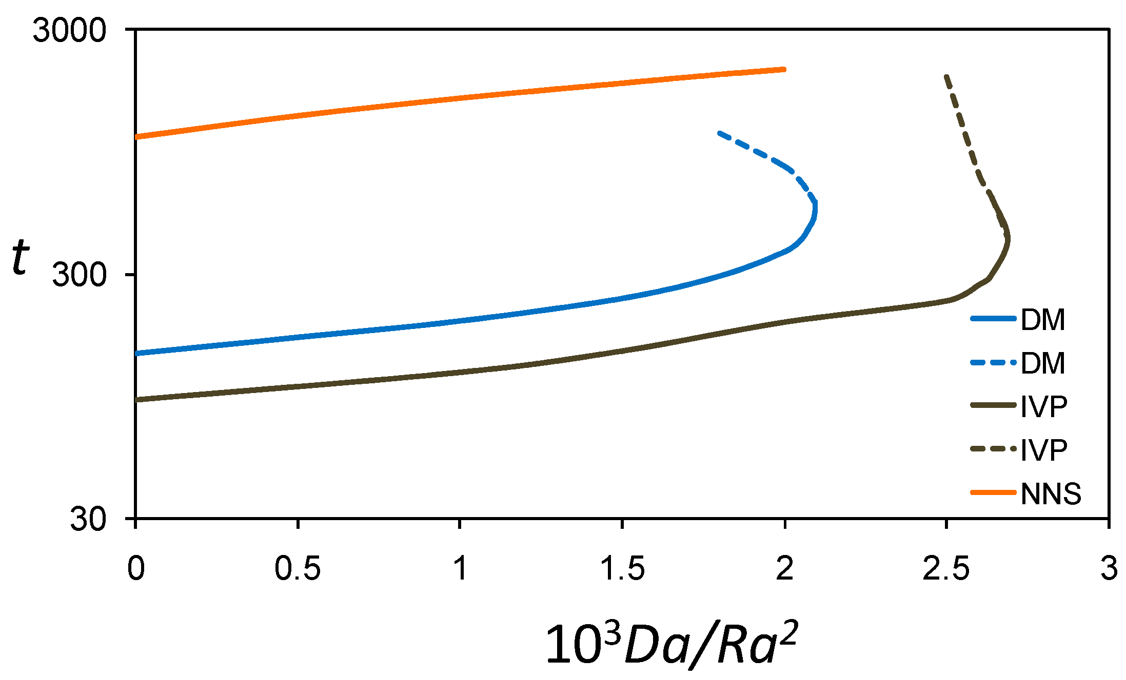
Figure 9.
The most unstable wave number at the onset of instability (dimensionless) as a function of for a precipitating reaction, predicted using the dominant mode analysis (DM), the initial-value problem approach (IVP), and the quasi-steady state assumption (QSSA).
Figure 9.
The most unstable wave number at the onset of instability (dimensionless) as a function of for a precipitating reaction, predicted using the dominant mode analysis (DM), the initial-value problem approach (IVP), and the quasi-steady state assumption (QSSA).

© 2017 by the authors. Licensee MDPI, Basel, Switzerland. This article is an open access article distributed under the terms and conditions of the Creative Commons Attribution (CC BY) license (http://creativecommons.org/licenses/by/4.0/).
Share and Cite
MDPI and ACS Style
Ghoshal, P.; Kim, M.C.; Cardoso, S.S.S. Onset of Convection in the Presence of a Precipitation Reaction in a Porous Medium: A Comparison of Linear Stability and Numerical Approaches. Fluids 2018, 3, 1. https://doi.org/10.3390/fluids3010001
AMA Style
Ghoshal P, Kim MC, Cardoso SSS. Onset of Convection in the Presence of a Precipitation Reaction in a Porous Medium: A Comparison of Linear Stability and Numerical Approaches. Fluids. 2018; 3(1):1. https://doi.org/10.3390/fluids3010001
Chicago/Turabian StyleGhoshal, Parama, Min Chan Kim, and Silvana S. S. Cardoso. 2018. "Onset of Convection in the Presence of a Precipitation Reaction in a Porous Medium: A Comparison of Linear Stability and Numerical Approaches" Fluids 3, no. 1: 1. https://doi.org/10.3390/fluids3010001