The Reduced NS-α Model for Incompressible Flow: A Review of Recent Progress

1
Department of Mathematics, Florida Polytechnic University, Lakeland, FL 33805, USA
2
Department of Mathematical Sciences, Clemson University, Clemson, SC 29634, USA
*
Author to whom correspondence should be addressed.
Fluids 2017, 2(3), 38; https://doi.org/10.3390/fluids2030038
Submission received: 3 June 2017
/
Revised: 19 June 2017
/
Accepted: 30 June 2017
/
Published: 6 July 2017
(This article belongs to the Special Issue Turbulence: Numerical Analysis, Modelling and Simulation)
Abstract
:This paper gives a review of recent results for the reduced Navier–Stokes- (rNS-) model of incompressible flow. The model was recently developed as a numerical approximation to the well known Navier–Stokes- model, for the purpose of more efficiently computations in the finite element setting. Its performance in initial numerical tests was remarkable, which led to analytical studies and further numerical tests, all of which provided excellent results. This paper reviews the main results established thus far for rNS-, and presents some open problems for future work.
1. Introduction
This paper presents a review of results for the recently introduced reduced Navier–Stokes- (rNS-) model of incompressible, viscous flow, given by
where w represents velocity, p a Bernoulli-type pressure, f a body force, and D a deconvolution operator intended to approximate the inverse of the Helmholtz (also called ) differential filter . The parameter > 0 represents the filtering radius.
For simplicity, only van Cittert approximate deconvolution,
is considered herein. This is the most common type used in fluid flow modeling [1,2,3]. Other types of approximate deconvolution operators, such as Tikhonov–Lavrentiev, may yield similar results, but all numerical tests done to date for rNS- have used van Cittert. Some advantages of van Cittert, which likely make it the most common, are that it is simple to use, easy to analyze, is formally very high accuracy, and has performed very well in many computational tests for several models [1,2,3]. Note that the groundbreaking idea of using approximate deconvolution in fluid models is due to Stolz, Adams and Kleiser [4,5,6,7]. Typically N is chosen small, and for all numerical simulations run so far with rNS-, 2.
The rNS- model was proposed in [8] as a numerical approximation to the well-known NS- model (see e.g., [9,10,11,12]) that is more efficiently computable in a finite element framework. NS- is given by
This model (also known as Camassa–Holm equations [11,12,13]) has extensive and attractive theoretical properties (see [9,10] and references therein), including well-posedness [10], frame invariance [14], adherence to Kelvin’s circulation theorem [9], conserving a model energy and helicity [9], requiring significantly fewer degrees of freedom than direct numerical simulation (DNS) of Navier–Stokes [9], and accurately predicting scalings of the turbulent boundary layer [15]. Most other fluid models do not have all (or even most) of these properties, and thus NS- is widely considered to be a very ‘physically accurate’ model. However, how to construct stable, efficient algorithms for it in the finite element setting is an open problem. The essential issue is that the filtering seemingly cannot be decoupled from the momentum-mass system in a stable way, leaving the practitioner to solve the nonlinear problem at each time step. Not only does this create the need for many system solves at each time step, but if one wishes to use a Newton iteration, then the linear systems must solve simultaneously for the velocity, filtered velocity, and pressure. However, rNS- can be computed efficiently in this setting, in the sense that it can stably decouple the filtering from the mass/momentum system, solve only one mass/momentum system at each time step, and obtain optimal accuracy. Initial testing of rNS- in [8,16,17] revealed outstanding results for turbulent channel flow simulation and flow past a cylinder.
The purpose of this paper is to review the recent analytical and numerical results for rNS-. In Section 2, the derivation of the model is shown and how it is related to other models and stabilizations. Section 3 reviews the analytical results established for the model, including a priori bounds, energy trapping, global well-posedness, energy dissipation rate, and energy spectra. Results for sensitivity of the model with respect to the filtering radius are discussed in Section 4. Numerical schemes and their analysis are given in Section 5, both for rNS- and its associated sensitivity equations from Section 4. Finally, in Section 6, results of numerical tests for channel flow past a cylinder and turbulent channel flow are discussed. Section 7 presents some open problems for possible future work.
2. Derivation of the Model and Connections to Other Models
It will be helpful for the later discussion to present the derivation found in [8] of the rNS- model, which starts from the NS- model. Recall from above that the NS- model is defined as follows, after writing :
It is discussed in detail in [8] why this model is difficult to efficiently compute with in a finite element framework.
The rNS- model is created through a series of transformations to NS-, as follows. By using in NS-, one gets
Denote , which provides
Next, use the approximation of the deconvolution operator, i.e., that , to get the rNS- model, written in terms of w and p after renaming variables due to the approximation:
2.1. Connections to Other Models
There are several models closely related to rNS- that have been studied recently, including NS- [9,11,12,13,18,19], NS–Voigt [20,21,22], and various other regularization models. It is important to make connections between the different models when possible, so existing results of various models can be fully utilized. It is clear from Equations (1)–(3) with , that for any N, choosing recovers the Navier–Stokes equations. Thus, if a mesh sufficient for a DNS of Navier–Stokes is used with rNS- and is chosen on the order of the mesh width, then the solution is expected to match the Navier–Stokes solution closely.
Deconvolution theory from [2] shows that formally recovers NS-, and the choice recovers the NS–Voigt model [20,21,22]. Hence, one can interpret the rNS- model as being ‘in between’ NS- and NS–Voigt, in the sense of deconvolution order. These connections are summarized in the following Table 1.
A second important connection for rNS- is to the generalized -models studied in [23]. By replacing w with and using the notation of [23], rNS- fits the general form with , , , and . Work done for these models reveals their strengths and weaknesses, and thus identifying connections between models is critical, as they can be extended to rNS-. For example, the main arguments in [8] for well-posedness of rNS- are similar to those made for NS–Voigt in [22,24].
When compared to other -models, rNS- has displayed better results on wall bounded turbulence, as demonstrated in [8,16,25]. A key difference between these models lies in the viscous term, which has the form instead of the standard . At the continuous level, the rNS- viscosity provides no extra smoothing, but it does provide additional dispersion when compared to the standard viscous term. This is due to the fact that , and this can be seen at high wave numbers since here [2].
Further insight is gained by expanding the deconvolution operator of the viscous term. Following [26], one can write
where can be considered as fluctuations about the (filtered) mean velocity [1]. In Equation (8), the ‘extra’ term reveals a connection to variational multiscale models (VMMs). It takes the form of a viscosity for velocity fluctuations, which is in the same spirit as VMMs, but differs in that here fluctuations are defined with filtered quantities as means. Interestingly, similar dissipation/penalty/stabilizations for the advection equation [27] and in turbulence simulations [28] were recently considered. These were also constructed by using filtering to define means and fluctuations, and have proven to be very successful at increasing accuracy of simulations on coarse discretizations.
One can also observe the effect of the extra term on the energy balance. Assuming periodic or no-slip boundary conditions for both the velocity and filtered velocities and using Equation (9), test rNS- with w to obtain
and using the filter definition yields the energy equality (from regularity results in [8], all operations are justified)
This demonstrates the effect on the energy dissipation, which serves to dissipate higher order norms of . Applying the filter definition once again, one can write
which more clearly shows that this extra viscous term acts to dissipate velocity fluctuations.
3. Analytical Results
The first analysis of rNS- was performed in [8], where it was shown that the model is well-posed for a fixed end time, and that regularity of solutions depended on the regularity of the data. Global in time energy and regularity results were proven in [17], and are stated below, after some initial preliminaries. The treatment of energy by the model was studied in [16]. Results for the energy conservation of the model, energy spectra, and energy dissipation were all very good: an appropriate energy quantity is conserved, the model exhibits a energy cascade on the large scales in the inertial range and at on smaller scales. Furthermore, energy is dissipated at the rate , independent of the Reynolds number, which is consistent with true fluid flow.
Consider in this section a domain , d = 2 or 3, which is a box. The notation and denotes the norm and inner product, with all other norms being labeled clearly. Assume periodic boundary conditions on the box, which is the common setting for such energy studies, as it is typically the only case where well-posedness of solutions is known. For the energy balance and dissipation results, the results extend to the wall-bounded case if the well-posedness results also extend to the wall-bounded case, which is an open problem. The energy spectra results, however, rely heavily on the periodic setting, as they explicitly use Fourier decompositions. Most of the filtering and deconvolution results can be extended to the case of homogeneous Dirichlet boundary conditions, if filtered velocities satisfy no-slip boundary conditions. This is not widely accepted as a correct boundary condition for the filter (on the other hand, this is the boundary condition use in all successful turbulent flow simulations with rNS- [8,16], and seems to work quite well).
Denote the periodic, zero-mean velocity and pressure spaces. The space is the dual space of X.
3.1. Energy Bounds and Well-Posedness
Presented now are several long time energy bounds. The following was proven in [17], and shows the energy is trapped for all times if and .
Lemma 1 (Energy trapping)
Suppose and . Then, ,
where . Thus, the kinetic energy is contained in the ball for all time.
Under the additional restriction that , then energy must decay to 0. This is proven in [17], and stated in the following lemma.
Lemma 2 (Energy decay)
Suppose and . Then, the energy decays to zero as :
Global well-posedness of the model was able to be proven, using the long time a priori energy bounds above [17].
Lemma 3 (Existence and uniqueness of weak solutions)
Suppose or and . Then, there exists a global unique weak solution to Equations (1)–(3).
Additional regularity of the data leads to global in time higher order regularity of solutions, and is proven in [17].
Lemma 4 (Higher order estimates)
Assume a solenoidal initial condition . If , then . If , then as .
Remark 1.
Assuming higher order regularity of the data, higher order regularity of solutions can be established using bootstrapping and the techniques used in [17].
3.2. Energy and Helicity Balances
Integral invariants such as energy and helicity are fundamental for a priori estimates used in existence theorems. They can also provide physical insight into a model’s behavior, as well as its physical relevance. It has long been established that these quantities are invariant in true fluid flow (i.e., in the Navier–Stokes equations), and as they are believed to be fundamental to the organization of flow structures, a good model should capture these quantities accurately.
The conserved model energy and helicity take the form:
The energy of this model is the same as for NS–Voigt [22]. As w represents an approximation of , with v being the NS- velocity, one can observe that the rNS- energy is analogous to the NS- energy ([9,10]). By similar reasoning, the rNS- helicity is connected to the NS–Voigt helicity and NS- helicity.
It is stated below, and proven in [16], that the energy and helicity of the model are preserved. Furthermore, if the forcing is only spatially dependent, then the energy balance leads to a global in time bound on energy.
Theorem 1.
Let w be the solution to Equations (1)–(3) under periodic boundary conditions, with sufficiently smooth data. Then, the following model energy and helicity balances hold:
In the case with vanishing viscosity and no external forcing, the model energy and helicity are exactly conserved. That is, for and ,
If the forcing is only spatially dependent, the energy balance from Theorem 1 can be further analyzed, revealing that is the energy dissipation of the model. The following result is proven in [16].
Suppose that the forcing is solenoidal and only dependent on space, , and the initial condition . Then,
3.3. Energy Dissipation Rate
Consider now the rate of energy dissipation by the model, and assume a constant solenoidal forcing, i.e., , and . The scale of the body force, large scale velocity, and length are defined as:
where denotes the time average. It can be shown that each component of the definition for L has units of length.
The following theorem for the scaling of the time averaged energy dissipation is proven in [16]. Recall that N is assumed small, i.e., .
Theorem 2.
The time averaged energy dissipation of the rNS-α model is bounded as
where is a constant dependent only on N (e.g., when ).
3.4. Energy Spectra
It is a generally accepted theory in turbulence that energy is input at large scales, cascaded (but preserved) by the nonlinearity through the ‘inertial range’ of intermediate scales, and then dissipated exponentially fast by viscosity in the small scale range. For accurate computations, it is critical to resolve the flow to where viscosity takes over. For the Navier–Stokes equations, resolving all of these scales is a computationally intractable problem, and it is necessary to model. Studying the energy spectra of a model allows us to gain insight into its computability, as a successful model must have an inertial range that is shorter than that of the Navier–Stokes. The analysis and notation below follows studies done in [9,34,35,36].
Decomposing velocity into its Fourier modes yields the balance of energy
where is the Fourier transform of , and
with
The quantity represents net energy transferred into the wave numbers between . Time averaging the balance Equation (15) gives the energy transfer equation
Define the model energy of a size eddy, based on the rNS- model energy , as
and combining with Equation (16) gives
with the last relation coming from [2]: for sufficiently large k. This is a key estimate for determining the inertial range, since here one expects no leakage of energy through dissipation, and hence . This suggests that increasing N leads to a shorter inertial range, which is consistent with the energy spectrum computations in Section 4.
The inertial range’s kinetic energy distribution is now considered. Begin by defining the average velocity of a size eddy, and then relate it to model energy:
From the Kraichnan energy cascade theory [37], one obtains that the eddy turnover time is
and thus the model energy dissipation rate scales like
Solving for , one obtains the relation
and this yields a spectrum for kinetic energy ():
Split the spectrum into two parts: if , then
but if ,
These scalings show that on larger inertial range scales, a rolloff of energy is expected (which agrees with true fluid flow). However, for wave numbers bigger than , a rolloff of is expected. These rolloffs are identical to usual NS- on both the larger and smaller scales in the inertial range [9]. This implies that significantly less energy is held in higher wave numbers compared to a Navier–Stokes DNS, which makes the model more computable than the Navier-Stokes Equations (NSE). Numerical tests in [16] illustrate these scalings. Another important takeaway is that since the rolloffs mirror those of NS-, one should expect computational cost (in terms of mesh width resolution) to be very similar NS-, at least in this periodic setting. This means that total cost in the finite element setting should be much less for rNS- compared to NS-, since the former is more efficiently computable, as discussed above.
4. Sensitivity of the Model with Respect to the Filtering Radius
The parameter in rNS- represents a filtering radius, and changing in computations can lead to very different solutions. Error analysis of the model’s discretization above suggests is a good choice, and choosing much smaller than this would lead to no regularization, since such a discrete filter would effectively have 0 filtering radius. Throughout the literature, is often chosen slightly larger than h, such as 2 h or 6 h (our experience makes us favor the choice of 2 h). Due to these various choices, it makes sense to study sensitivity of the model to changes in , and in this section, a sensitivity equation for is derived and analyzed. In later sections, efficient algorithms are proposed for computing it, and finally computations are performed. This section follows work done in [17].
The sensitivity equation for is derived by applying to rNS-, then setting and . This gives
This system is reduced by eliminating variables for filtered velocities’ sensitivities after evaluating , and writing the system in terms of . The system depends on N, and for the first few values of N, one gets
| N | ||
| 0 | I | |
| 1 | ||
| 2 | ||
| 3 |
Note that for general N, one can write can be written as plus a linear combination of filtered w’s,
where the ’s are integers depending on N. Thus, the general system takes the form
This system is proven in [17] to be well-posed in the periodic setting, and the result reads as follows:
Theorem 3 (Existence and uniqueness of weak sensitivity solutions)
In the numerical tests section below, efficient numerical schemes for computing this sensitivity system are proposed and analyzed.
5. Numerical Schemes and Analysis
An efficient numerical scheme for approximating solutions to rNS- using a finite element spatial discretization, together with an implicit-explicit BDF2 timestepping, is given. This time discretization linearizes the system at each time step and decouples the filtering/deconvolution equations from the momentum/mass system. After providing some preliminaries, the scheme and results for its stability, well-posedness, and convergence, are presented.
5.1. Problem Setting and Preliminaries
Assume a regular, conforming triangulation/tetrahedralization , and associated inf-sup stable discrete velocity-pressure spaces that are piecewise polynomials on each element. Define the discretely divergence free subspace by
Discrete filtering is defined by the standard finite element discretization of the filter: Given , find satisfying
Discrete van Cittert deconvolution is analogous to the continuous case, but defined with the discrete filter:
An explicit filter operator is now given that filters known quantities exactly, but for unknown quantities, it instead filters a known second order approximation:
This operator defines an explicit deconvolution operator
Finally, the implicit-explicit (IMEX) BDF2, finite element scheme for the rNS- model can be stated.
| Algorithm 1: [BDF2] Given endtime , timestep , forcing , and initial velocities , set and for , find satisfying for all , |
5.2. Analysis of the Scheme
Results of the stability and convergence of Algorithm 1 are now stated, and come from [8].
Lemma 5 (Stability)
Suppose that . Then solutions of Algorithm 1 satisfy
Moreover, solutions to Algorithm 1 exist uniquely since the scheme is linear at each timestep. Thus, the algorithm is well-posed.
Remark 3.
In most settings where large eddy simulation (LES) models such as rNS-α is used, it generally holds that . Moreover, typically 3, giving . Thus, in practice, the timestep restriction will typically be mild.
Convergence of the scheme is proven in [8] and is stated in the following theorem.
Theorem 4.
Suppose are chosen to be either Taylor–Hood elements or Scott–Vogelius elements and suppose further that is a solution of Equations (1) and (2) for a given , , with forcing and initial velocity , satisfying regularity criteria , , . Suppose further that the stability criterion for the timestep size is satisfied. Then the error of Algorithm 1 in approximating solutions to the rNS-α model satisfies
5.3. Numerical Scheme for rNS- Sensitivity
An efficient numerical scheme is now detailed for the rNS- sensitivity system to be used together with the IMEX BDF2 scheme above. The key feature for efficiency is that the discrete velocity/pressure and sensitivity systems will have exactly the same coefficient matrices. Thus, preconditioners for the velocity solve can be reused, and also one can take advantage of block solvers that work with multiple right-hand sides, since the proposed algorithms allows solving for and simultaneously. The discrete scheme is now presented. Step 1 is exactly the rNS- scheme from above. Step 2 solves for velocity and pressure sensitivity, and is decoupled from Step 1.
| Algorithm 2: [rNS- with sensitivity] Given , , , and timestep , for , |
| Step 1: Find satisfying: |
| Step 2: Find satisfying: |
Stability and convergence of the Step 1 is stated above, and it is proven in [17] that Step 2 is stable and convergent. However, there is a slightly more restrictive condition on the time step size.
Theorem 5.
Let , , and choose such that . Then,
Furthermore, assuming sufficiently smooth data, the convergence estimate holds:
6. Numerical Results
Results of computations for rNS- are presented in this section. First, results of convergence rate tests are given, to illustrate the convergence results above. Next, two application problems are considered, 2D flow past a cylinder and 3D turbulent channel flow. For the two application problems, comparisons of the model solutions to the literature are made, and sensitivities are also computed and discussed.
6.1. Verification of Convergence Rates
In [8], convergence rate verification tests were performed for the IMEX scheme above for rNS-. The test problem used was an exact rNS- solution (i.e., it solves (1) and (2) with ) given by
where is defined for each N by (justification of the existence of such a constant is given in [8]).
Approximations to this exact solution were calculated in [8] on and , using Algorithm 1, with , , , , and (with ). Errors and rates for the scheme were computed, using successively refined uniform meshes and timesteps, with Taylor–Hood elements. Based on Theorem 4, convergence is expected to satisfy
Thus, a convergence rate of 2 is predicted if the mesh width and the time step are reduced together, by a factor of 2 at each refinement, which is observed to be the case from Table 2.
6.2. 2D Channel Flow Past a Cylinder
Results of tests of the rNS- model/scheme for 2D flow past a cylinder are now presented. This is a benchmark problem from [38,39,40], with the domain being a 2.2 × 0.41 rectangular channel with a radius = 0.05 cylinder, centered at , as shown in Figure 1. No slip boundary conditions are prescribed on the walls and cylinder, and the inflow and outflow profiles are given by
The kinematic viscosity is set as , the forcing , and the flow starts from rest. The correct behavior is for a vortex street to form by t = 4 and continue to t = 8. The flow is driven by an interaction of the fluid with the cylinder, which is an important scenario for industrial flows. This flow is not turbulent, but is still very challenging for most numerical models and methods, especially on coarser meshes.
Important statistics for this flow are the predicted lift and drag forces. For a velocity field u and pressure p, lift and drag coefficients are defined by
where is tangential velocity, is the max velocity at the inlet, , , S is the cylinder, and is the outward unit normal.
Solutions were computed using Algorithm 1 with and elements on a very coarse barycenter mesh that provided 5104 velocity degrees of freedom (dof). This choice of elements is made because the model is implemented using a Bernoulli-type pressure, which is significantly more complex than usual pressure and is known to affect the overall error if standard element choices are used [41], but not if divergence-free elements are used. The deconvolution parameter was chosen, and tests were run with varying from to . To evaluate these solutions, values for the maximum drag and lift coefficients were calculated, and compared to those found in the resolved benchmark tests of [42]:
For comparison, the max lift and drag coefficient values were calculated on the same mesh, elements, and time step by the NSE discretized by the following extrapolated Crank–Nicolson finite element method:
One observes from Table 3 that rNS- provides much better max lift and drag coefficients than the coarse mesh NSE. The reference values come from upwards of dof simulations, and it is remarkable the rNS- gets this level of accuracy on such a coarse discretization.
6.2.1. Sensitivity to in Flow Past a Cylinder
For this test problem, sensitivity of the solution to was considered, and Algorithm 2 was computed with = 0.001, = 0.001, and Scott–Vogelius elements on a barycenter refined Delaunay triangulation, which provided 35,948 total dof. Plots of the sensitivity magnitude are shown in Figure 2 at various times. At early times, the sensitivity is created at the cylinder, and then as time progresses, it gets convected into the flow. By t = 6, values of are near 600. Creation of sensitivity at the solid boundary is not unexpected, since the sensitivity equation resembles a vorticity equation.
Lift and drag sensitivities are also calculated, defined by differentiating the lift and drag formulas above with respect to . For the tests above, these quantities are also calculated:
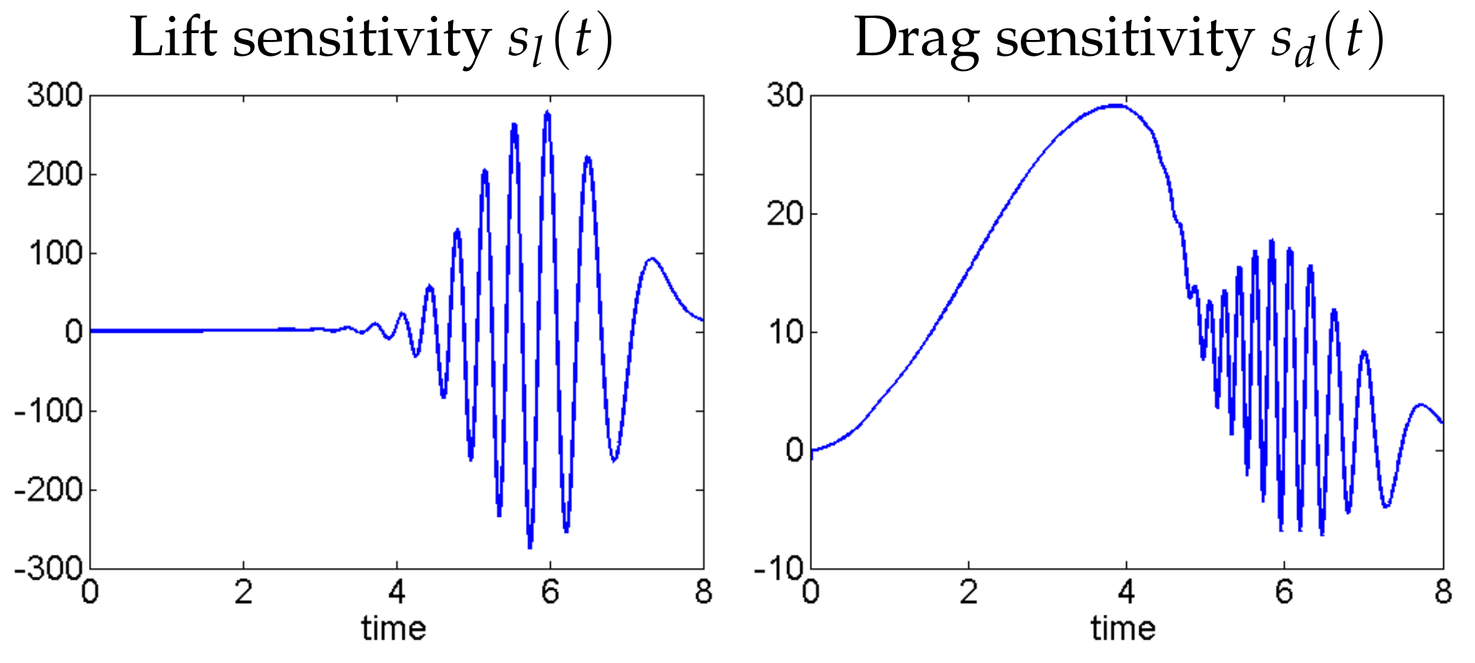
Here, denotes the tangential sensitivity. Shown in Figure 3 are plots of and versus time that came from this test. One observes very large sensitivity with the lift, and less so in the drag, but still significant. One also observes that the drag sensitivity is positive for most of the simulation, indicating that increasing will increase drag.
6.3. Turbulent Channel Flow at = 590
Results from rNS- tests on a benchmark turbulent channel flow problem with friction Reynolds number = 590 from [16] are now discussed. The results below show that rNS- does an outstanding job at matching the DNS mean velocity profile on a very coarse mesh. To our knowledge, no other model produces results this good on such a coarse mesh. For the widely cited DNS results [43], the number of degrees of freedom used was 113 million (our tests use just 82,821). For comparison, results on the same discretization for Leray-, NS-, and NS–Voigt models were computed on the same coarse mesh in [16] and shown to be much worse than rNS-.
6.3.1. Problem Description and Results
The problem setup is given in detail in [8,16,44], and the interested reader is referred to those works for additional details. The domain is the box , with homogeneous Dirichlet boundary conditions enforced on the top and bottom walls and , and periodic boundary conditions enforced on the remaining sides. The kinematic viscosity is set at . The initial condition is created by randomly perturbing the DNS average velocity profile pointwise. These perturbations create the turbulence as the simulation is run. The forcing is defined by , and is dynamically adjusted at each time step to maintain the bulk velocity. The simulations are run to t = 60, and the time and space average of the velocity is done from t = 20 to t = 60.
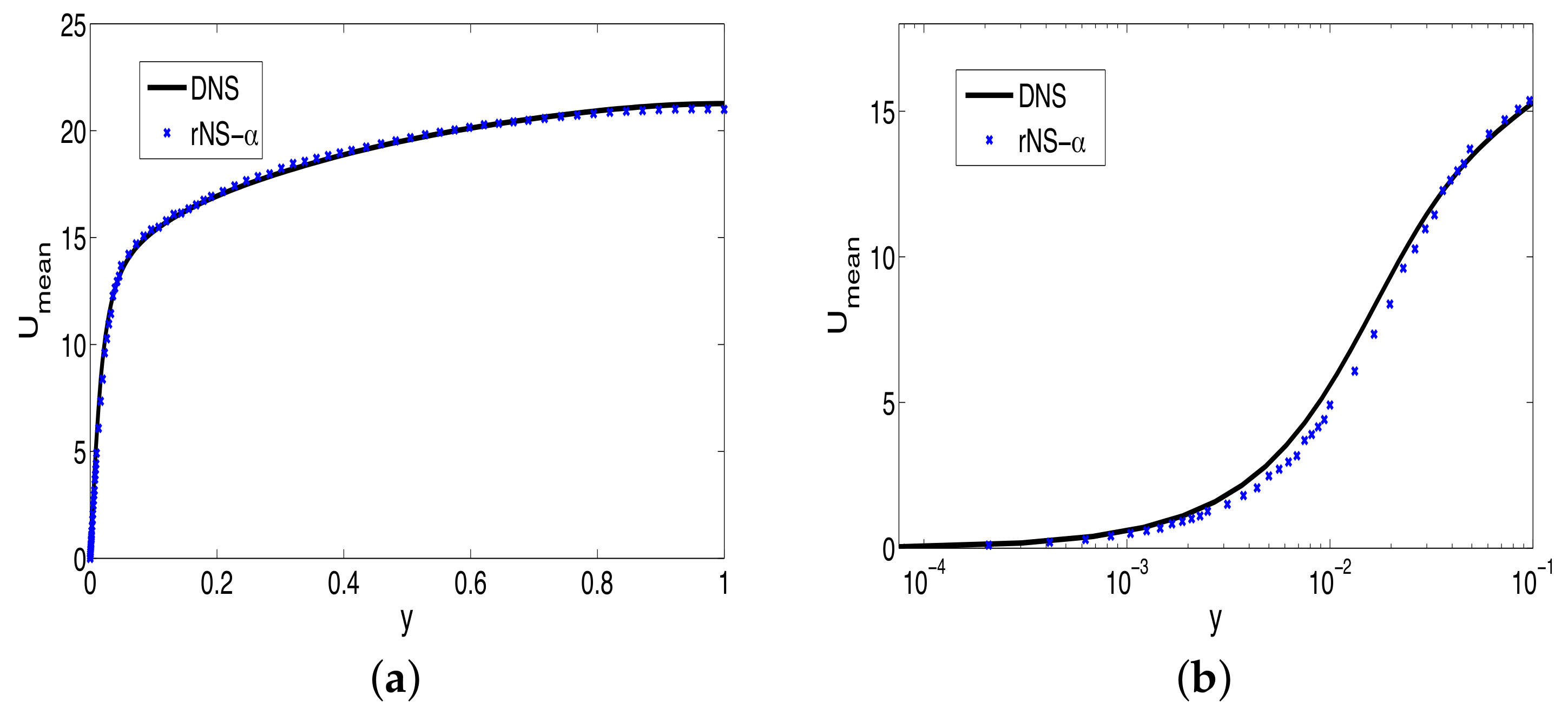
divergence-free Scott–Vogelius elements are used with a barycentric tetrahedral mesh that is weighted towards the walls, and provides 82,821 velocity dof. The time step size , deconvolution N = 2, was varied. The value of gives an optimal (to within 0.0005) solution in the sense of best matching the DNS mean velocity profile; note that this value is close to the mesh resolution near the wall. Mean streamwise velocity profiles for rNS- are shown in Figure 4, together with DNS data. Results this good are seemingly unique for any regularization model on such a coarse mesh, using a finite element discretization.
The difference between the DNS mean streamwise velocity, and various model’s mean streamwise velocity, is shown in Table 4 (the values of are optimal to within 0.0005 in the interval [0,0.1] One immediately observes the rNS- is much more accurate than Leray- and NS–Voigt (which both barely improve on the ‘no model’, i.e., NSE on the coarse mesh). NS- blows up for each choice of (note the nonlinear problem was not solved at each time step; instead, a linearization on the filtered term in the nonlinearity is done, to make its efficiency the same as the other models (see [16])).
6.4. Model Sensitivity for Turbulent Channel Flow with = 590
rNS- sensitivity was tested in [17] for this benchmark turbulent channel flow problem. Since the quantity of interest for this problem is the long time averaged velocity, a sensitivity study of rNS- for this problem is now performed, to determine the long time averaged velocity sensitivity.
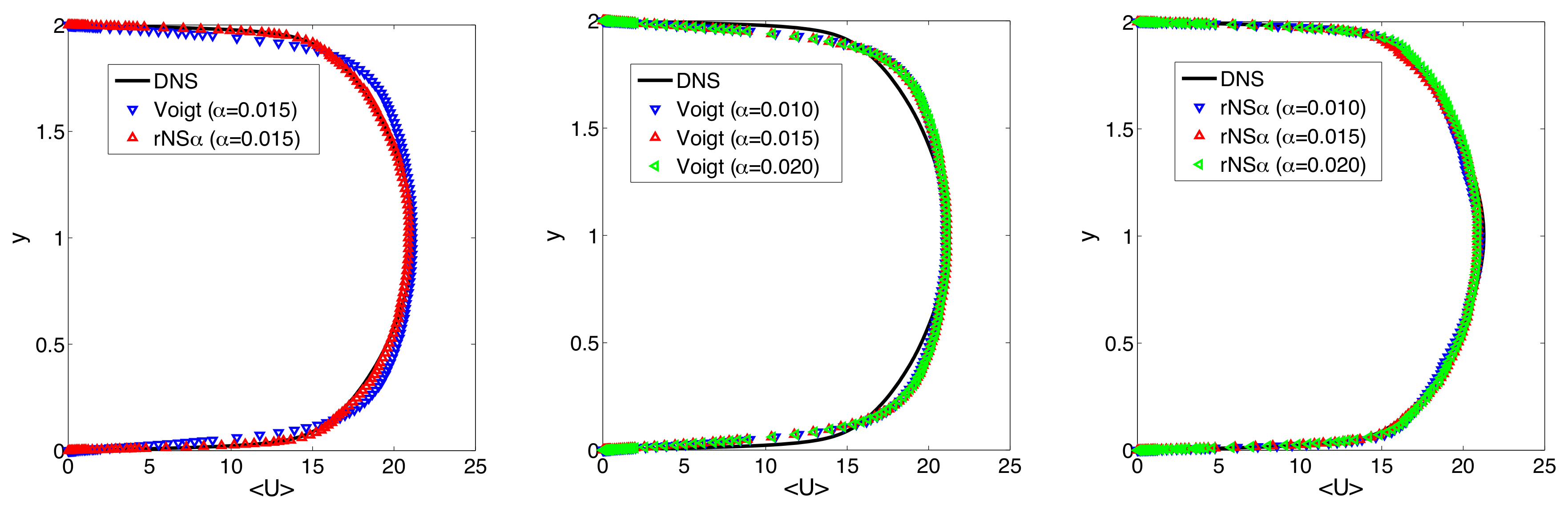
The same discretization as in [16] is used for this test: decoupled IMEX-BDF2-finite element discretization (step 1 of Algorithm 2), and Scott–Vogelius elements on a tetrahedral mesh that provided 82,281 velocity (and sensitivity) degrees of freedom. Both and (which is the NS–Voigt model) are tested, and = 0.010, 0.015 and 0.020. Starting from the T = 60, , (turbulent) solution as the initial condition (created using the setup above), the simulation is run to T = 70 s using a time step size of (1000 total time steps). Algorithm 2 step 2 is used to calculate sensitivities at each time step, and time and space (x and z directions) averages are taken to get the mean streamwise velocity and sensitivity profiles.
From Figure 5, observe that rNS- () gives an excellent prediction of the mean streamwise velocity profile for each choice of , significantly better than the NS–Voigt () case. For the varying , there is no visible change in the NS–Voigt solution, and a slight visible change in the rNS- solution.
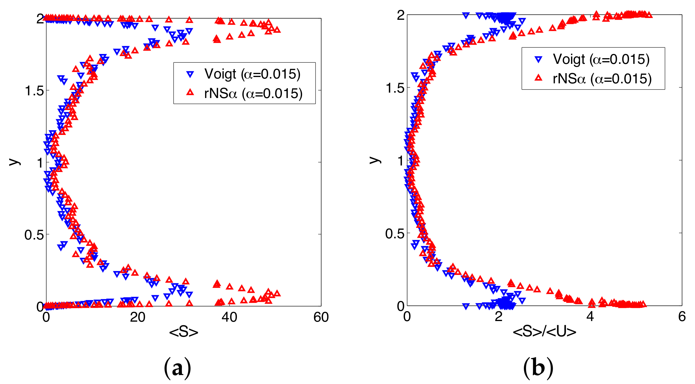
Figure 6 shows the mean streamwise sensitivity and relative sensitivity magnitudes, for both rNS- and NS–Voigt. One observes that rNS- is more sensitive than NS–Voigt to changes in . More interesting is the observation that the sensitivity is largest near the boundary. Although this is perhaps expected due to (1) the boundary layer is critical for turbulent channel flow; and (2) the ‘correct’ boundary conditions for filtered velocities is an open problem for LES/ models (note the N = 0 model does not use filtered velocity boundary conditions).
7. Conclusions
The main results to date for rNS- have been reviewed in this paper. This includes global well-posedness, energy spectrum analysis, and energy dissipation analysis. An efficient numerical discretization is reviewed, and corresponding stability and convergence results are given. Additionally, sensitivity equations for rNS- are derived, and a numerical scheme for them is given. Finally, results of several numerical tests are given, which show excellent results on several benchmark problems.
There are several directions for future work. Further testing, further comparison to other LES models, and exploration of the model outside of the finite element framework should all be done. One could also immediately move this model into the multiphysics arena, for non-isothermal flow, or doubly diffusive flow, or even to magnetohydrodynamics. Additional numerical testing on difficult benchmark problems is also important for any newer models. An interesting study could likely be done for rNS-’s near-wall behavior; it remains unclear what makes rNS- so much more accurate for turbulent channel flow, but one hypothesis is that it could be more accurate near the wall. Another interesting future direction of this work is to consider the rNS- model, but remove all modeling except in the viscous term. That is, one could consider a simplified model to be
or possibly keep the Voigt term . Proceeding as in Section 2, one can write the momentum equation of this reduced model as
Note that this system can be considered as Navier–Stokes with an additional term meant to dissipate velocity fluctuations. Our discussion in Section 2 shows that the altered viscous term is strongly related to the VMM approach to turbulence modeling, so it is possible that it is only this term that is to thank for the model’s successes on the turbulent channel flow benchmark tests. One also notes that implementing the term would require very little extra work in a simulation, if the velocity term is treated implicitly and the filtered velocity is treated explicitly (by extrapolating from previous time steps).
Author Contributions
Abigail L. Bowers and Leo G. Rebholz did an equal amount of work on this manuscript, including the analysis, experiments, and writeup.
Conflicts of Interest
The authors declare no conflict of interest.
References
- Berselli, L.; Iliescu, T.; Layton, W. Mathematics of Large Eddy Simulation of Turbulent Flows; Scientific Computation; Springer: Berlin, Germany, 2006. [Google Scholar]
- Chacon-Rebello, T.; Lewandowski, R. Mathematical and Numerical Foundations of Turbulence Models and Applications; Springer: New York, NY, USA, 2014. [Google Scholar]
- Layton, W.; Rebholz, L. Approximate Deconvolution Models of Turbulence: Analysis, Phenomenology and Numerical Analysis; Springer: Berlin, Germany, 2012. [Google Scholar]
- Stolz, S.; Adams, N.; Kleiser, L. The approximate deconvolution model for large-eddy simulations of compressible flows and its application to shock-turbulent-boundary-layer interaction. Phys. Fluids 2001. [Google Scholar] [CrossRef]
- Adams, N.; Stolz, S. A subgrid-scale deconvolution approach for shock capturing. J. Comput. Phys. 2002, 178, 391–426. [Google Scholar] [CrossRef]
- Adams, N.A.; Stolz, S. On the approximate deconvolution procedure for LES. Phys. Fluids 1999, 2, 1699–1701. [Google Scholar]
- Stolz, S.; Adams, N.; Kleiser, L. An approximate deconvolution model for large-eddy simulations with application to incompressible wall-bounded flows. Phys. Fluids 2001, 13, 997–1015. [Google Scholar] [CrossRef]
- Cuff, V.; Dunca, A.; Manica, C.; Rebholz, L. The reduced order NS-α model for incompressible flow: Theory, numerical analysis and benchmark testing. ESAIM Math. Model. Numer. Anal. 2015, 49, 641–662. [Google Scholar] [CrossRef]
- Foias, C.; Holm, D.; Titi, E. The Navier–Stokes-alpha model of fluid turbulence. Physica D 2001, 152, 505–519. [Google Scholar] [CrossRef]
- Foias, C.; Holm, D.; Titi, E. The three dimensional viscous Camassa–Holm equations, and their relation to the Navier–Stokes equations and turbulence theory. J. Dyn. Differ. Equ. 2002, 14, 1–35. [Google Scholar] [CrossRef]
- Chen, S.; Foias, C.; Holm, D.; Olson, E.; Titi, E.; Wynne, S. The Camassa–Holm equations as a closure model for turbulent channel and pipe flow. Phys. Rev. Lett. 1998, 81, 5338–5341. [Google Scholar] [CrossRef]
- Chen, S.; Foias, C.; Olson, E.; Titi, E.; Wynne, W. The Camassa-Holm equations and turbulence. Physica D 1999, 133, 49–65. [Google Scholar] [CrossRef]
- Chen, S.; Foias, C.; Olson, E.; Titi, E.; Wynne, W. A connection between the Camassa-Holm equations and turbulent flows in channels and pipes. Phys. Fluids 1999, 11, 2343–2353. [Google Scholar] [CrossRef]
- Guermond, J.; Oden, J.; Prudhomme, S. An interpretation of the Navier–Stokes-alpha model as a frame-indifferent Leray regularization. Physica D 2003, 177, 23–30. [Google Scholar] [CrossRef]
- Cheskidov, A. Boundary layer for the Navier–Stokes-α model of fluid turbulence. Arch. Ration. Mech. Anal. 2004, 172, 333–362. [Google Scholar] [CrossRef]
- Rebholz, L.; Kim, T.Y.; Byon, Y.L. On an accurate α model for coarse mesh turbulent channel flow simulation. Appl. Math. Model. 2017, 43, 139–154. [Google Scholar] [CrossRef]
- Rebholz, L.; Zerfas, C.; Zhao, K. Global in time analysis and sensitivity analysis for the reduced NS-α model of incompressible flow. J. Math. Fluid Mech. 2016, 1–23. [Google Scholar] [CrossRef]
- Kim, T.Y.; Cassiani, M.; Albertson, J.; Dolbow, J.; Fried, E.; Gurtin, M. Impact of the inherent separation of scales in the Navier–Stokes-αβ equations. Phys. Rev. E 2009, 79045307, 1–4. [Google Scholar]
- Kim, T.Y.; Neda, M.; Rebholz, L.; Fried, E. A numerical study of the Navier–Stokes-αβ model. Comput. Methods Appl. Mech. Eng. 2011, 200, 2891–2902. [Google Scholar] [CrossRef]
- Kalantarov, V.; Titi, E. Global attractors and determining modes for the 3D Navier–Stokes-Voight equations. Chin. Ann. Math. Ser. B 2009, 30, 697–714. [Google Scholar] [CrossRef]
- Levant, B.; Ramos, F.; Titi, E. On the statistical properties of the 3D incompressible Navier–Stokes-Voigt model. Commun. Math. Sci. 2010, 8, 277–293. [Google Scholar] [CrossRef]
- Larios, A.; Titi, E. On the higher-order global regularity of the inviscid Voigt-regularization of three-dimensional hydrodynamic models. Discret. Contin. Dyn. Syst. 2010, 14, 603–627. [Google Scholar]
- Holst, M.; Lunasin, E.; Tsogtgerel, G. Analytical study of generalized α-models of turbulence. J. Nonlinear Sci. 2010, 20, 523–567. [Google Scholar] [CrossRef]
- Berselli, L.C.; Bisconti, L. On the structural stability of the Euler-Voight and Navier-Stokes-Voight models. Nonlinear Anal. 2012, 75, 117–130. [Google Scholar] [CrossRef]
- Abdi, N. TurBulence Modelling of the Navier–Stokes Equations Using The NS-α Approach. Master’s Thesis, Freie Universitat, Berlin, Germany, 2015. [Google Scholar]
- Dunca, A.; Epshteyn, Y. On the Stolz-Adams deconvolution model for the large-eddy simulation of turbulent flows. SIAM J. Math. Anal. 2005, 37, 1890–1902. [Google Scholar] [CrossRef]
- Dunca, A.; Neda, M. On the Vreman filter based stabilization for the advection equation. Appl. Math. Comput. 2015, 269, 379–388. [Google Scholar] [CrossRef]
- Vreman, A. The filtering analog of the variational multiscale method in large-eddy simulation. Phys. Fluids 2003, 15, 1–5. [Google Scholar] [CrossRef]
- Frisch, U. Turbulence; Cambridge University Press: Cambridge, UK, 1995. [Google Scholar]
- Constantin, P.; Doering, C. Energy Dissipation in Shear Driven Turbulence. Phys. Rev. Lett. 1992, 69, 1648–1651. [Google Scholar]
- Constantin, P.; Doering, C. Variational Bounds on Energy Dissipation in Incompressible Flows: Shear Flow. Phys. Rev. E 1994, 49, 4087–4099. [Google Scholar]
- Doering, C.R.; Gibbon, J.D. Applied Analysis of the Navier–Stokes Equations; Cambridge University Press: Cambridge, UK, 1995. [Google Scholar]
- Layton, W.; Rebholz, L.; Sussman, M. Energy and helicity dissipation rates of the NS-alpha and NS-alpha-deconvolution models. IMA J. Appl. Math. 2010, 75, 56–74. [Google Scholar] [CrossRef]
- Berselli, L.; Kim, T.Y.; Rebholz, L. Analysis of a reduced-order approximate deconvolution model and its interpretation as a NS–Voigt regularization. DCDS-B 2016, 21, 1027–1050. [Google Scholar] [CrossRef]
- Cao, Y.; Lunasin, E.; Titi, E. Global well-posedness of the three-dimensional viscous and inviscid simplified Bardina turbulence models. Commun. Math. Sci. 2006, 4, 823–848. [Google Scholar] [CrossRef]
- Cheskidov, A.; Holm, D.; Olson, E.; Titi, E. On a Leray-α model of turbulence. Proc. R. Soc. A 2005, 461, 629–649. [Google Scholar] [CrossRef]
- Kraichnan, R. Inertial-range transfer in two- and three-dimensional turbulence. J. Fluid Mech. 1971, 47, 525. [Google Scholar] [CrossRef]
- John, V. Reference values for drag and lift of a two dimensional time-dependent flow around a cylinder. Int. J. Numerical Methods Fluids 2004, 44, 777–788. [Google Scholar] [CrossRef]
- Schäfer, M.; Turek, S. The benchmark problem ‘flow around a cylinder’ flow simulation with high performance computers II. In Notes on Numerical Fluid Mechanics; Hirschel, E.H., Ed.; Vieweg: Braunschweig, Germany, 1996; Volume 52, pp. 547–566. [Google Scholar]
- Hannasch, D.; Neda, M. On the accuracy of the viscous form in simulations of incompressible flow problems. Numer. Methods Partial Differ. Equ. 2012, 28, 523–541. [Google Scholar] [CrossRef]
- John, V.; Linke, A.; Merdon, C.; Neilan, M.; Rebholz, L.G. On the divergence constraint in mixed finite element methods for incompressible flows. SIAM Rev. 2017, in press. [Google Scholar]
- John, V.; Rang, J. Adaptive time step control for the incompressible Navier–Stokes equations. Comput. Methods Appl. Mech. Eng. 2010, 199, 514–524. [Google Scholar] [CrossRef]
- Moser, R.; Kim, J.; Mansour, N. Direct numerical simulation of turbulent channel flow up to Reτ = 590. Phys. Fluids 1999, 11, 943–945. [Google Scholar] [CrossRef]
- John, V.; Roland, M. Simulations of the turbulent channel flow at Reτ = 180 with projection-based finite element variational multiscale methods. Int. J. Numer. Methods Fluids 2007, 55, 407–429. [Google Scholar] [CrossRef]
- Galvin, K.; Rebholz, L.; Trenchea, C. Efficient, unconditionally stable, and optimally accurate FE algorithms for approximate deconvolution models. SIAM J. Numer. Anal. 2014, 52, 678–707. [Google Scholar] [CrossRef]
- Bowers, A.; Rebholz, L. Numerical study of a regularization model for incompressible flow with deconvolution-based adaptive nonlinear filtering. Comput. Methods Appl. Mech. Eng. 2013, 258, 1–12. [Google Scholar] [CrossRef]
- Layton, W.; Rebholz, L.; Trenchea, C. Modular nonlinear filter stabilization of methods for higher Reynolds numbers flow. J. Math. Fluid. Mech. 2012, 14, 325–354. [Google Scholar] [CrossRef]
Figure 1.
Shown above is the channel flow around a cylinder domain.
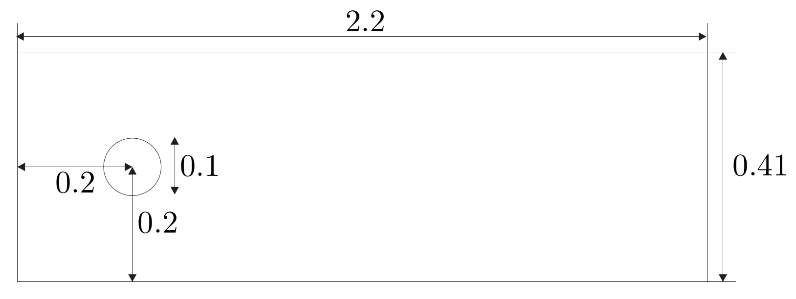
Figure 2.
Sensitivity magnitudes at various times.
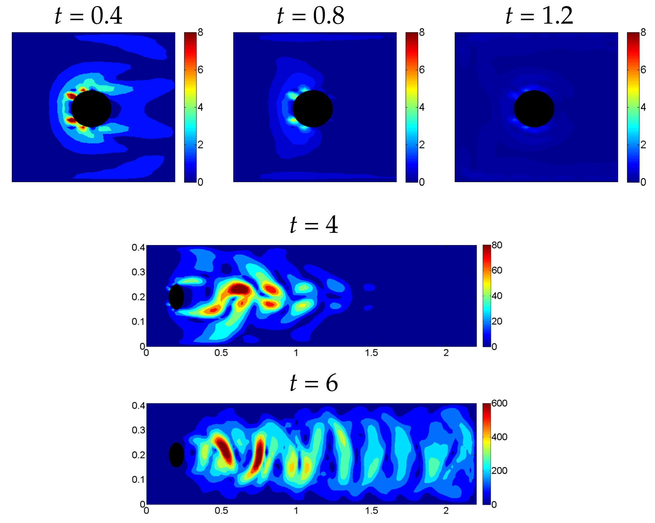
Figure 3.
Sensitivities of lift and drag coefficients, plotted with time.

Figure 4.
Shown above are the average velocity profiles of the coarse mesh reduced Navier–Stokes- (rNS-) simulation and direct numerical simulation (DNS) of the Navier-Stokes Equations (NSE), at = 590, shown in regular coordinates in (a), and near the wall in a log scale in (b).
Figure 4.
Shown above are the average velocity profiles of the coarse mesh reduced Navier–Stokes- (rNS-) simulation and direct numerical simulation (DNS) of the Navier-Stokes Equations (NSE), at = 590, shown in regular coordinates in (a), and near the wall in a log scale in (b).

Figure 5.
Average streamwise velocity profiles for DNS, rNS-, and NS–Voigt models.

Figure 6.
Average streamwise sensitivity (a) and relative streamwise sensitivity magnitude (b) for rNS- and Voigt solutions with = 0.015.
Figure 6.
Average streamwise sensitivity (a) and relative streamwise sensitivity magnitude (b) for rNS- and Voigt solutions with = 0.015.


Table 1.
Connections summary.
| N | rNS- Model Reduces to | |
|---|---|---|
| 0 | Navier–Stokes | |
| >0 | 0 | NS–Voigt |
| >0 | ∞ | NS- |
Table 2.
Velocity errors and rates for the convergence rate test are given in the table, and are consistent with the optimal theoretical rate of 2.
Table 2.
Velocity errors and rates for the convergence rate test are given in the table, and are consistent with the optimal theoretical rate of 2.
| h | Rate | ||
|---|---|---|---|
| 1/4 | 1/2 | 1.005 | - |
| 1/8 | 1/4 | 6.553 | 0.617 |
| 1/16 | 1/8 | 1.678 | 1.965 |
| 1/32 | 1/16 | 4.089 | 2.037 |
| 1/64 | 1/32 | 1.141 | 1.841 |
Table 3.
Shown in the table are max lift and drag coefficients for various models and parameters, for 2D flow past a cylinder.
Table 3.
Shown in the table are max lift and drag coefficients for various models and parameters, for 2D flow past a cylinder.
| Model | % Error | % Error | |||
|---|---|---|---|---|---|
| Navier–Stokes (NS) | - | 3.393 | 15.0% | 0.7499 | 56.9% |
| rNS- | 0.011 | 3.074 | 4.2% | 0.511 | 6.9% |
| rNS- | 0.012 | 3.107 | 5.2% | 0.506 | 5.9% |
| rNS- | 0.013 | 3.142 | 6.4% | 0.501 | 4.8% |
| rNS- | 0.014 | 3.180 | 7.8% | 0.497 | 4.0% |
| rNS- | 0.015 | 3.220 | 9.2% | 0.492 | 3.0% |
| rNS- | 0.016 | 3.264 | 10.6% | 0.487 | 1.9% |
Table 4.
The difference between the model’s predicted velocity profile and the (cubic spline of) Moser, Kim, and Moin velocity profile for = 590, using results from the model with optimal from 0.001 to 0.070, with increments of 0.001. No NS- simulation with the implicit-explicit (IMEX) algorithm from the appendix remained stable for the entire simulation.
| = 590 | ||
|---|---|---|
| Model | Optimal | |
| Navier-Stokes Equations (NSE) coarse mesh | - | 1.409 |
| rNS- | 0.012 | 0.184 |
| NS- | DNE | DNE |
| Leray- | 0.040 | 1.213 |
| NS–Voigt | 0.030 | 1.238 |
© 2017 by the authors. Licensee MDPI, Basel, Switzerland. This article is an open access article distributed under the terms and conditions of the Creative Commons Attribution (CC BY) license (http://creativecommons.org/licenses/by/4.0/).
Share and Cite
MDPI and ACS Style
Bowers, A.L.; Rebholz, L.G. The Reduced NS-α Model for Incompressible Flow: A Review of Recent Progress. Fluids 2017, 2, 38. https://doi.org/10.3390/fluids2030038
AMA Style
Bowers AL, Rebholz LG. The Reduced NS-α Model for Incompressible Flow: A Review of Recent Progress. Fluids. 2017; 2(3):38. https://doi.org/10.3390/fluids2030038
Chicago/Turabian StyleBowers, Abigail L., and Leo G. Rebholz. 2017. "The Reduced NS-α Model for Incompressible Flow: A Review of Recent Progress" Fluids 2, no. 3: 38. https://doi.org/10.3390/fluids2030038