Baseline Model for Bubbly Flows: Simulation of Monodisperse Flow in Pipes of Different Diameters

Abstract

CFD simulations of the multiphase flow in technical equipment are feasible within the framework of interpenetrating continua, the so-called two-fluid modelling. Predictions with multiphase CFD are only possible if a fixed set of closures for the interfacial exchange terms is available that has been validated for a wide range of flow conditions and can therefore reliably be used also for unknown flow problems. To this end, a baseline model, which is applicable for adiabatic bubbly flow, has been specified recently and has been implemented in OpenFOAM. In this work, we compare simulation results obtained using the baseline model with three different sets of experimental data for dispersed gas-liquid pipe flow. Air and water under similar flow conditions have been used in the different experiments, so that the main difference between the experiments is the variation of the pipe diameter from 25 mm to 200 mm. Gas fraction and liquid velocity are reasonably well reproduced, in particular in the bulk of the flow. Discrepancies can be seen in the turbulent kinetic energy, the gas velocity and in the wall peaks of the gas fraction. These can partly be explained by the simplified modelling, but to some extent must be attributed to uncertainty in the experimental data. The need for improved near-wall modelling, turbulence modelling and modelling of the bubble size distribution is highlighted.

1. Introduction

Many technical processes in industries, such as chemical or electricity, but also numerous natural phenomena involve multiphase flow. A wide range of relevant length scales and complex physics make it a formidable task to achieve a better understanding of such flows. Multiphase computational fluid dynamics can be a valuable tool for analysis and prediction, as one can get a detailed insight into the local flow field. In this way, CFD potentially could contribute greatly to the optimization of existing and the development of new processes, respectively process equipment.

For technical equipment, CFD simulations are possible within the Eulerian two-fluid framework of interpenetrating continua. In this framework, the details of the flow on the small length scale of the disperse phase are eliminated due to an averaging procedure. This relaxes the requirements on the grid resolution and, hence, facilitates computations on large domains. On the other hand, the interfacial transfer of momentum, mass and heat occurring on the small scales needs to be modelled by suitable closure relations.

Even when heat and mass transfer are excluded, a large number of works exist on the application of two-fluid models to a specific flow problem using different closure relations of varying degrees of sophistication. Systems that are of considerable practical interest and have therefore been considered particularly extensively are bubble columns [1,2,3] and bubbly pipe flows [4,5]. The relevance of various forces acting on the bubbles and suitable correlations describing their strength depending on the local flow parameters have been assessed [6,7,8,9]. Different general frameworks for the description of turbulence have been compared [6,7,10,11,12,13], and a number of possibilities to include the bubble-induced contribution to the turbulence have been considered [10,14,15,16]. Several available frameworks to include processes of bubble coalescence and breakup have been applied [17,18,19,20,21], and specific expressions for the rates of these processes have been employed [22,23]. Finally, the effect of an additional solid phase present in the flow domain, e.g., in slurry bubble column reactors or flotation columns, on the hydrodynamics and on coalescence and breakup has been studied recently [24,25,26].

Despite this large body of works, no complete, reliable and robust formulation has been achieved so far, which is probably due to the fact that in each investigation, largely a different set of closure relations is compared to a different set of experimental data. The resulting lack of generality of each of the proposed models is aggravated when the closures employed contain parameters that are only determined by matching the validation data. Accurate and trustworthy predictions, however, require a set of closures that works without fine-tuning constants to a specific problem, but that has been validated for a broad range of physical properties and flow conditions.

Since the closure relations are formulated in terms of local field variables, one may expect that in as much as the physics governing the processes occurring on small scale is the same, the same closure relations should apply irrespective of the large-scale geometry and boundary conditions. Hence, it should indeed be possible to cover a broad range of applications in a unified manner without the necessity for case by case tuning. Consequently, a baseline model applicable for adiabatic bubbly flows was defined based on the best available current knowledge. Following this baseline strategy, the model has successfully been validated against experimental data for upward vertical pipe flow [27,28,29] and for fluid dynamics in bubble columns [30,31] using the commercial code ANSYS CFX.

Model validation should be done for well-defined experiments in which local properties of both phases have been measured, in which for the least the phase fraction, the velocities of both phases, fluctuating velocities, and the size (distribution) of the disperse phase were measured. This is of great importance, as the closure relations for the different physical phenomena that have to be modelled, such as bubble forces, bubble-induced turbulence and coalescence and breakup, interact in a complex way. In the validation process, it is desirable to consider cases where some of these coupled effects are known to be only of minor importance and, therefore, allowing for the reduction of the model complexity. In this way, the remaining submodels for the other effects may be validated independently. An example of this procedure, which has been used previously and is continued here, is to substitute measured values for the bubble size to bypass models for bubble coalescence and breakup, which are still in a less mature state than those for bubble forces and bubble-induced turbulence.

In principle, the closures model the underlying physical phenomena, and hence, the baseline model should be equally applicable in other CFD software. However, even though the same set of closures was implemented in the open source software package OpenFOAM in Rzehak and Kriebitzsch [32], some differences were observed compared to the results of Rzehak and Krepper [27], and one empirical parameter had to be changed to obtain comparable agreement with the experimental data with both codes. The validation of this approach is extended in the present contribution.

To this end, simulations are performed of the experiments provided by Shawkat et al. [33] and by Hosokawa and Tomiyama [34], which are here for the first time simulated using the baseline model. In a previous investigation, these experiments were used to assess the models for bubble-induced turbulence, however with different closures for the bubble forces than later included in the baseline model [35]. These two datasets nicely complement our previous studies [32], which considered two-phase flow in pipes with a diameter of approximately 50 mm studied experimentally by Liu [36]. Together, the data from all three experimental works form a comprehensive database on bubbly flows in pipes of different diameters, namely 25 mm, approximately 50 mm and 200 mm, for the data of Hosokawa and Tomiyama [34], Liu [36] and Shawkat et al. [33], respectively. At the same time, other parameters, like gas and liquid superficial velocities, bubble diameters and material properties, are comparable in all works. For the sake of a coherent presentation of the model validation for the complete database, some repetition of previously-obtained results seems justified.

The paper is organized as follows. In Section 2, we summarize the test cases and data used for the simulations. We briefly describe the model, boundary conditions and simulation settings in Section 3. Subsequently, we compare the simulation results obtained with our baseline model against the experimental data in Section 4. Based on the findings in Section 4, we critically review currently available drag force closures and available experimental data for the slip velocity in bubbly pipe flow in Section 5. Finally, we draw conclusions concerning the performance of the baseline model and identify further research directions to improve the baseline model and broaden its range of applicability.

2. Summary of the Experimental Data

2.1. Tests of Liu [36]

The system studied by Liu [36] is the vertical up-flow of water and air in a round pipe with inner diameter D = 57.2 mm. They performed experiments specifically designed to show the effects of bubble size by using a special gas injector that allows adjusting the bubble size independent of liquid and gas mass fluxes. All three parameters, average bubble size <d_B>, liquid mass flux J_L and gas mass flux J_G, were varied in the investigation. Radial profiles of gas fraction α_G, bubble-size d_B, axial liquid velocity u_L and axial liquid turbulence intensity u_L’ were measured at an axial position L/D = 60, so that fully-developed flow conditions are realized. The average bubble diameter was computed in that work from measurements of the chord length using a dual needle resistivity probe based on the assumption of a spherical shape of the bubble. A change in the gas fraction profile from wall to core peak with increasing bubble size was observed, as well as turbulence suppression in the pipe center for combinations of high liquid and low gas mass flux, which correspond to the smallest bubble sizes. Lacking a precise specification, pressure and temperature presumably are at ambient conditions. An overview of the major characteristics of the test cases selected for the present work is given in

Table 1. Overview of the major characteristics of the selected test cases, where the letter “H” denotes the experimental data provided by Hosokawa and Tomiyama [34], “L” the cases of Liu [36], and “S” refers to the data of Shawkat et al. [33]. Nominal values are as reported in the quoted references, and adjusted values are obtained as described in Section 3.5.

Name	Pipe Diameter	JL (nom)	JG (nom)	JL (adj)	JG (adj)	<dB>	<αG>
	mm	m/s	m/s	m/s	m/s	mm	%
H11	25.0	0.5	0.018	0.5	0.018	3.2	2.5
H12	25.0	0.5	0.025	0.5	0.031	4.3	4.1
H21	25.0	1.0	0.020	1.0	0.035	3.5	2.8
H22	25.0	1.0	0.036	1.0	0.042	3.7	3.2
L11A	57.2	0.5	0.1	0.5	0.12	2.9	15.2
L21B	57.2	1.0	0.1	1.0	0.14	3.0	10.6
L21C	57.2	1.0	0.1	1.0	0.13	4.2	9.6
L22A	57.2	1.0	0.2	1.0	0.22	3.9	15.7
S21	200	0.45	0.015	0.41	0.019	4.1	2.4
S23	200	0.45	0.1	0.5	0.108	5.0	10.7
S31	200	0.68	0.015	0.67	0.018	3.2	1.7
S33	200	0.68	0.1	0.71	0.12	4.7	10.1

, where the letter “L” denotes the tests of Liu [36].

Wall-bounded turbulence is anisotropic, which means that components of the fluctuating velocity in axial, radial and azimuthal directions u’, v’ and w’ are different. Data on axial and radial components are given, e.g., in Michiyoshi and Serizawa [37], Wang et al. [38] or Shawkat et al. [33]. These works show that the axial component is always greater than or equal to the radial component. The ratio u’/v’ is largest near the pipe walls and for single-phase flow. Data on the azimuthal component for typical turbulent two-phase flow conditions could not be found in the literature. Concerning turbulent kinetic energy k, an estimate of the ratio √ k/u’ may be obtained from the quoted works by assuming that azimuthal and radial components are equal as √ k/u’ ≈ 0.8 … 1.2. The lower bound is a bit larger than the value √(1/2) ≈ 0.71 corresponding to the unidirectional limiting case, while the upper bound is almost the same as √(3/2) ≈ 1.22 obtained for isotropic turbulence. Taking u’ as an estimate for √ k thus provides an estimate that is accurate to within ~20%.

2.2. Tests of Shawkat et al. [33]

Shawkat et al. [33] conducted a study with varying liquid and gas mass fluxes in the vertical up-flow of water and air in a round pipe with inner diameter D = 200 mm. Radial profiles of the void-fraction, bubble-size, liquid, as well as gas velocities and axial, as well as radial liquid turbulence intensity and Reynolds-stress were measured at an axial position L/D = 42. Similar to [36], the average bubble diameter was computed in that work from measurements of the chord length based on the assumption of a spherical shape of the bubble, however using an optical dual needle probe. A change in the gas fraction profile from wall to core peak with increasing bubble size was observed, as well as turbulence suppression at the pipe wall for combinations of high liquid and low gas mass flux, which correspond to the smallest bubble sizes. The relevant parameters for the selected cases are denoted by the letter “S” in Table 1. By assuming that radial and azimuthal components of the velocity fluctuations are equal, an estimate of the turbulent kinetic energy is obtained. The average values for gas fraction and bubble diameter given in [33] are obtained from radial averaging of the profiles.

2.3. Tests of Hosokawa and Tomiyama [34]

Hosokawa and Tomiyama [34] is another study with some variation of liquid and gas mass fluxes in the vertical up-flow of water and air in a round pipe. Here, the pipe diameter D = 25.0 mm is rather small. Radial profiles of the void-fraction, liquid and gas velocity and liquid turbulent kinetic energy were measured at an axial position L/D = 68. In addition, the distribution of bubble sizes has been recorded. In that work, the equivalent spherical diameter was computed from a reconstruction of stereoscopic images. The minimum and maximum diameter that was measured was 2 mm, respectively 5 mm, for cases H11, H21 and H22 and 2 mm, respectively 8 mm, for case H23. However, for case H23, the fraction of bubbles larger than 5 mm is rather small. The data contain both wall and core peaking gas fraction profiles. Turbulence suppression is observed for the cases with high liquid velocity where in this case, no clear relation with bubble size can be discerned. The characteristic data of these measurements are shown in Table 1, denoted by the letter “H”.

3. Description of the Models

Concerning the conservation equations of the two-fluid model, a broad agreement has been reached, and the general form of the equations is discussed in several text books (e.g., [39,40,41]). However, there is no consensus on the closure relations, which are needed to complete the model equations to allow for the computation of actual flow problems.

In this work, we use the baseline model as described in detail in Rzehak and Kriebitzsch [32] and applied by the authors’ group to different flow problems, as shown in [28,29,30,31,42]. Therefore, we will only outline the most important aspects, and the interested reader is referred in particular to [32] for details.

3.1. Two-Fluid Model Equations

The conservation of mass for adiabatic flows is expressed as:

$$\frac{\partial }{\partial t}\left({\alpha }_G{\rho }_G\right)+\nabla \cdot \left({\alpha }_G{\rho }_G{\mathit{u}}_G\right)=0$$

(1)

$$\frac{\partial }{\partial t}\left({\alpha }_L{\rho }_L\right)+\nabla \cdot \left({\alpha }_L{\rho }_L{\mathit{u}}_L\right)=0$$

(2)

and for momentum:

$$\frac{\partial }{\partial t}({\alpha }_G{\rho }_G{\mathit{u}}_G)+\nabla \cdot ({\alpha }_G{\rho }_G{\mathit{u}}_G\otimes {\mathit{u}}_G)=-{\alpha }_g\nabla p+\nabla \cdot ({\alpha }_G{T}_G)+ {\alpha }_G{\rho }_G\mathit{g}+{\mathit{F}}_G^{inter}$$

(3)

$$\frac{\partial }{\partial t}({\alpha }_L{\rho }_L{\mathit{u}}_L)+\nabla \cdot ({\alpha }_L{\rho }_L{\mathit{u}}_L\otimes {\mathit{u}}_L)=-{\alpha }_L\nabla p+\nabla \cdot ({\alpha }_L{T}_L)+ {\alpha }_L{\rho }_L\mathit{g}+{\mathit{F}}_L^{inter}.$$

(4)

The equations above imply the so-called volume conservation, given by the constrained ${\alpha }_L+{\alpha }_G=1$.

The stress tensor T includes the viscous, as well as the Reynolds stresses. The volumetric interfacial force density ${\mathit{F}}_G^{inter}$ is modelled as a sum of different contributions:

$${\mathit{F}}_G^{inter}=-{\mathit{F}}_L^{inter}={\mathit{F}}^{drag}+{\mathit{F}}^{lift}+{\mathit{F}}^{wall}+{\mathit{F}}^{disp},$$

(5)

which are discussed in Section 3.2.

3.2. Bubble Forces

Based on our experience in the simulation of bubbly air-water pipe flow, we model the momentum exchange between both phases as a sum of the drag, lift, wall and turbulent dispersion forces.

The resistance the bubbles experience due to the relative motion with the liquid phase is described by the drag force. The standard approach:

$${\mathit{F}}^{drag}=-\frac{3}{4}{C}_D\frac{{\rho }_L{\alpha }_G}{d_B}\left|{\mathit{u}}_G-{\mathit{u}}_L\right|\left({\mathit{u}}_G-{\mathit{u}}_L\right)$$

(6)

is used to model this force density, with the drag coefficient C_D being computed from the correlation given by Ishii and Zuber [43].

A bubble moving in an unbounded shear flow experiences a force perpendicular to its direction of motion. This lift force is given by the force density:

$${\mathit{F}}^{lift}=-C_L{\rho }_L{\alpha }_G\left({\mathit{u}}_G-{\mathit{u}}_L\right)\times \left(\nabla \times {\mathit{u}}_L\right),$$

(7)

with the lift coefficient C_L. A correlation proposed by Tomiyama et al. [44] is used to estimate the lift coefficient C_L as a function of the Eötvös number.

When a bubble moves parallel to a wall, it experiences an additional force, the so-called wall lift force or simply wall force. This force is an effect of the modification of the flow field due to the presence of the wall as compared to a bubble rising in an infinite liquid, as a consequence of which the pressure distribution on the surface of the bubble is changed. As seen from the experiments of Hosokawa et al. [45], this force becomes active while the bubble is still some distance away from the wall. Its general form, written as a volumetric force density, is given as:

$${\mathit{F}}^{wall}=-C_W\frac{{\rho }_L{\alpha }_G}{d_B}{\left|{\mathit{u}}_G-{\mathit{u}}_L\right|}^2 \widehat{\mathit{y}}.$$

(8)

Based on a comparison given in [46], we use for the wall force coefficient C_W the correlation given by Hosokawa et al. [45]. Due to the small Morton number of the air-water system, log(Mo) = −10.6, we only use the Eötvös-dependent part given in [45].

Finally, the turbulent dispersion force accounts for the effect of the turbulent fluctuations of the liquid velocity on the bubbles. We employ the model proposed by Burns et al. [47]:

$${\mathit{F}}^{disp}=-C_{TD}\frac{3}{4}{C}_D\frac{{\rho }_L{\alpha }_G}{d_B}\left|{\mathit{u}}_G-{\mathit{u}}_L\right|\frac{{\mu }_L^{t\mathit{u}rb}}{{\sigma }_{TD}}\left(\frac{1}{{\alpha }_L}+\frac{1}{{\alpha }_G}\right)\nabla {\alpha }_G,$$

(9)

with the turbulent dispersion Schmidt number σ_TD and the turbulent dispersion force coefficient C_TD. A value of σ_TD = 0.9 is used, and the turbulent dispersion force coefficient is set to C_TD = 2.0.

We have not considered the virtual mass force, because we are simulating steady, fully-developed pipe flow. The importance of the virtual mass force in other types of flows has been discussed in the literature, e.g., [13,31,48].

One has to note that the approach of modelling the momentum exchange as a sum of different contributions is a simplification, which is strictly valid only for low bubble Reynolds numbers when the equations are linear. To the authors’ knowledge, no other approaches have been suggested in the published literature so far, and the available modelling work shows that this approach gives reliable results provided a thorough validation of the model.

3.3. Turbulence Modelling

Due to the small spatial scales of the dispersed gas and its low density, it suffices to model the turbulence of the continuous liquid phase. Like in the previous studies [27,35], we use an additional source term in the equations of the liquid phase turbulence model to account for the bubble-induced turbulence. Here, we adopt the Shear Stress Transport (SST) model of Menter [49], which is a two-equation Reynolds-averaged Navier-Stokes (RANS) model that combines the strengths of the k-ε and k-ω models. The equations for k and ε are augmented by source terms $S_L^k$ and $S_L^{\epsilon }$ modeling the bubble-induced turbulence. From a detailed comparison of different models for bubble-induced turbulence (Rzehak and Krepper [35]), the following expressions have emerged as the best choice:

$$S_L^k={\mathit{F}}^{drag}\cdot \left({\mathit{u}}_G-{\mathit{u}}_L\right)$$

(10)

and:

$$S_L^{\mathsf{\epsilon }}=\frac{\sqrt{k_L}}{d_B}{S}_L^k.$$

(11)

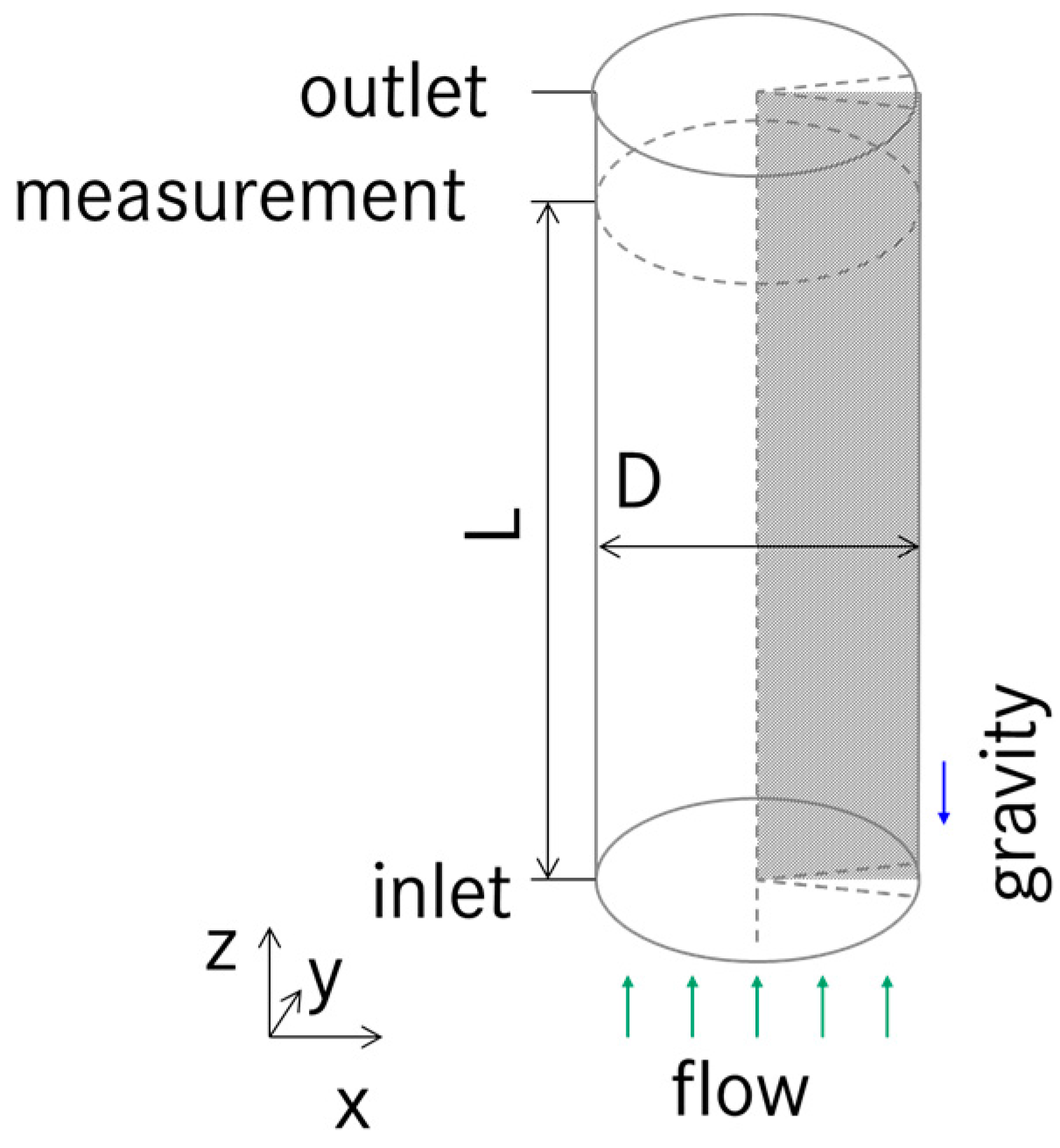
3.4. Geometry and Boundary Conditions

In our chosen approach of a Reynolds-averaged description, the flow is statistically axisymmetric. Hence, we use a quasi-2D cylindrical geometry in the simulations, as depicted in Figure 1. This means that we model only a narrow cylindrical sector, which has symmetry boundary conditions on its side faces. As shown in previous work (e.g., [27]), this simplification is valid for the type of flow considered in this work. A specific boundary condition called “wedge” is available in OpenFOAM to use this kind of simplification in CFD simulations [50].

At the bottom, the inlet condition for the liquid velocity is set to a typical single-phase turbulent flow profile in a pipe. The gas fraction is set to a uniform profile, and gas velocity is set to a shifted liquid velocity profile, such that the desired superficial gas velocity is obtained.

The turbulent kinetic energy k at the inlet is set based on the inlet velocity and a specified value for the turbulence intensity I_t:

$$k_{in}=\frac{3}{2}{\left(I_t\left|{\mathit{u}}_L\right|\right)}^2.$$

(12)

The turbulent frequency ω at the inlet is computed from the turbulent kinetic energy k_in and the turbulent length scale:

$${\omega }_{in}=\frac{C_{\mu }^{-1}{k}^{1/2}}{L_t}.$$

(13)

A value of 5% has been chosen for the turbulence intensity, and the turbulent length scale is prescribed as 10% of the pipe diameter. Modification of these values had no visible effect on the results. As long as fully-developed flow is attained at the measurement location, the precise inlet conditions do not matter, which has been checked by looking at the axially-resolved gas fraction fields.

To ensure that the outlet conditions do not influence the results at the measurement location, a flow abatement zone has been added atop the measurement plane with a length that is about 10% of the main flow section. We used a pressure boundary condition at the outlet. A no-slip boundary condition is specified for the liquid phase on the walls and a free-slip condition for the gas phase, assuming that the bubbles do not directly contact the walls.

To avoid the need to resolve the viscous sub-layer, we use a single-phase wall function for the turbulent kinetic energy k and for the turbulent frequency ω. This is based on the view that the liquid phase contacts the complete wall area and, hence, exerts the full shear stress on the walls. In the near-wall cell, ω is set from the analytical solution, and a zero-gradient condition normal to the wall is used for k.

3.5. Other Model Aspects

For the cases considered in this work, the bubble size is smaller than 5 mm. For such cases, a monodisperse approximation is appropriate and, therefore, also used in our simulations. We have used the average bubble diameters, which were measured in the experiments and which are given in Table 1, as the equivalent spherical diameter of the bubbles in our simulations.

In the simulations, both gas and liquid are assumed incompressible with the material properties being constant, which is different from the experiments where the bubble expand a bit while rising in the pipe due to the pressure drop. As discussed in [27], this deviation can be corrected by computing the gas flow rate from the measured values at the measurement location:

$$J_G=2 \pi {{\displaystyle \int }}_0^{\frac{D}{2}}{\alpha }_G\left(r\right) u_G\left(r\right) r dr.$$

(14)

If only the liquid velocity $u_L$ has been measured, one can compute the gas velocity $u_G$ from the liquid velocity assuming fully-developed stationary flow. The values of the adjusted gas fluxes $J_G$ (adj) are also given in Table 1.

The materials used in the experiments were air and water. In the simulations, the properties of these materials at 25 °C and atmospheric pressure are used, which are shown in

Table 2. Material properties for the air water system at atmospheric pressure and 25 °C temperature.

ρL	997.0	kg·m−3
µL	8.899 × 10 −4	kg m−1·s−1
ρG	1.185	kg·m−3
µG	1.831 × 10 −5	kg·m−1·s−1
σ	0.072	N·m−1

. Decreasing or increasing the temperature by five degrees has only a small effect on the value of the material properties.

4. Simulation Results

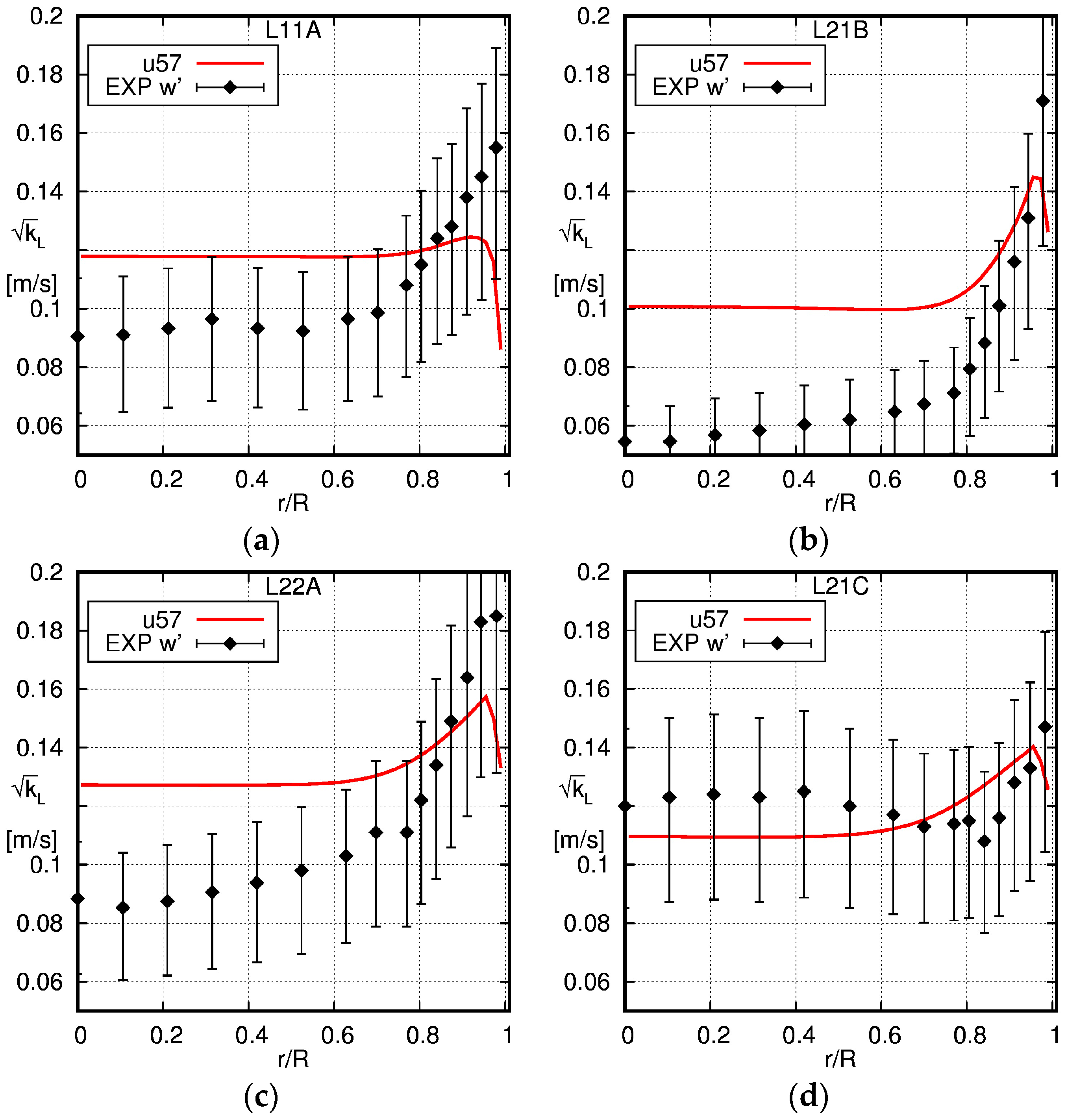
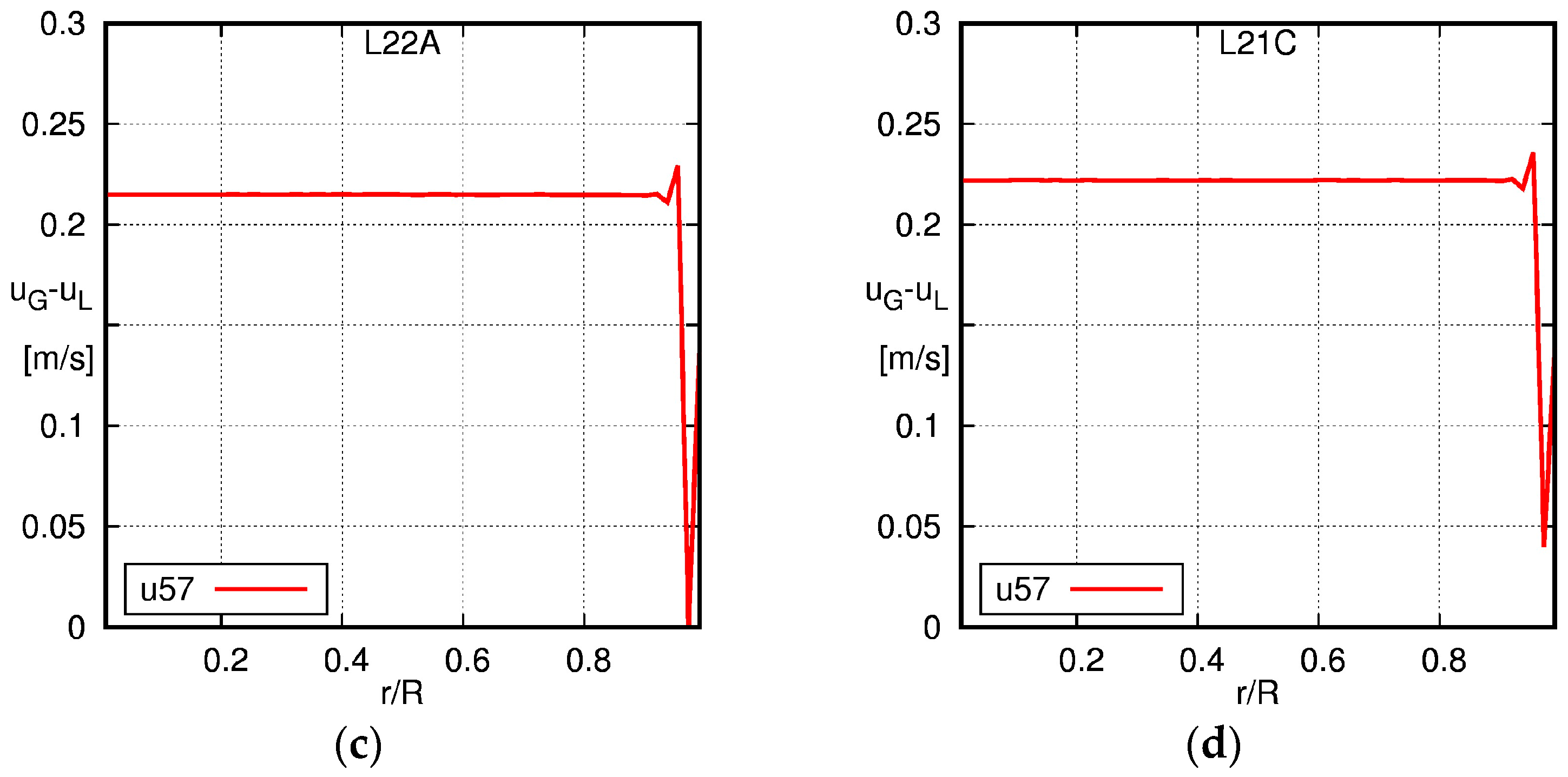
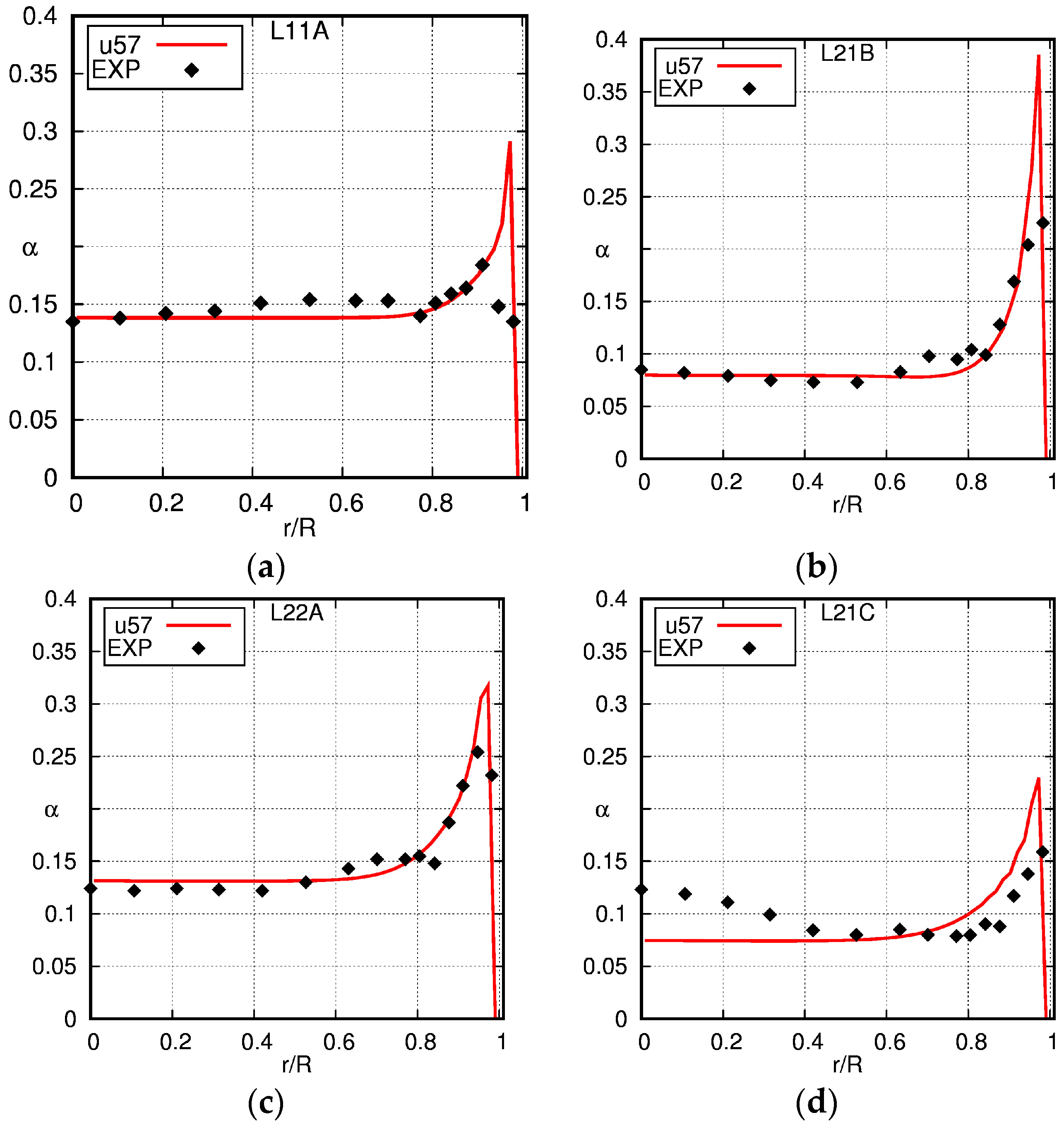
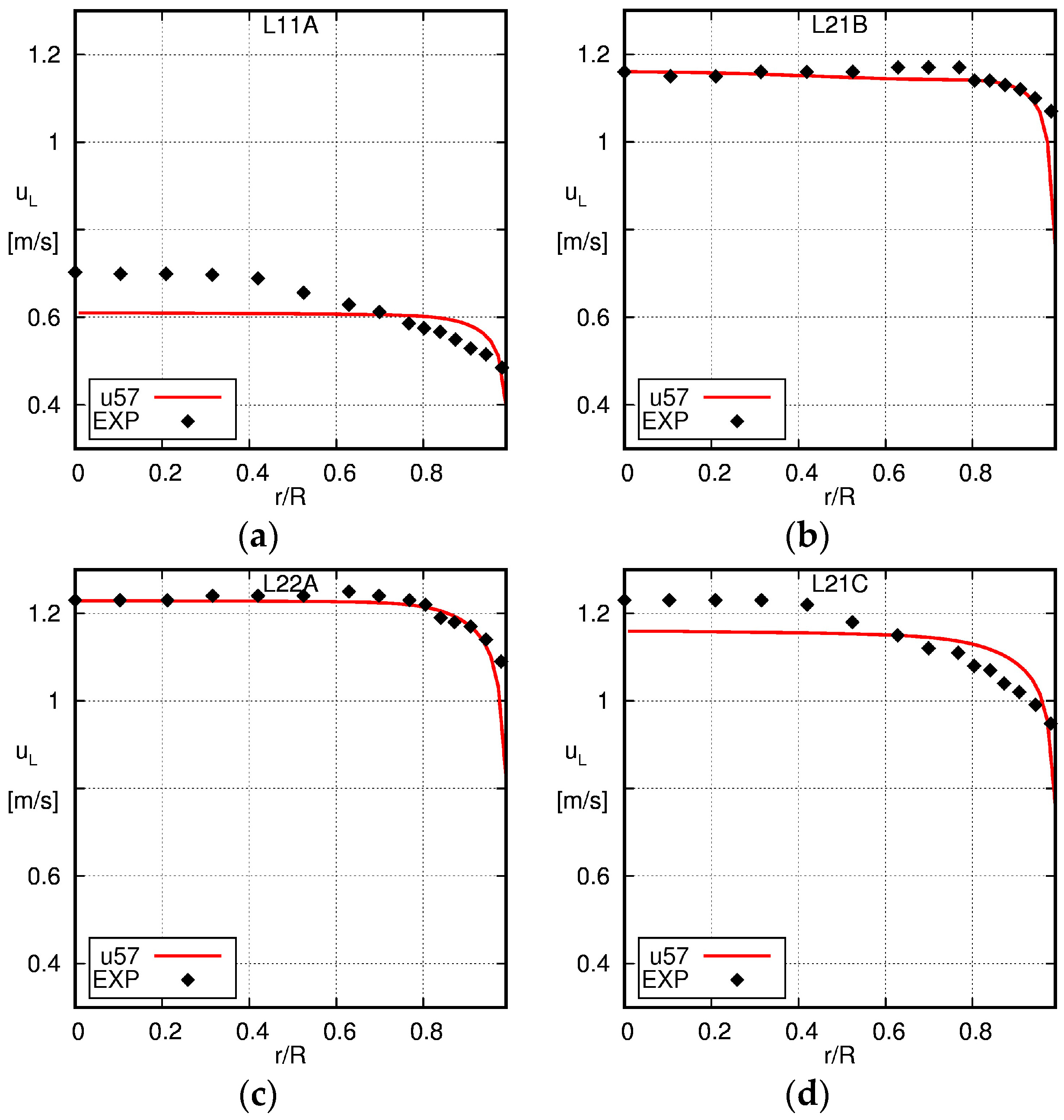
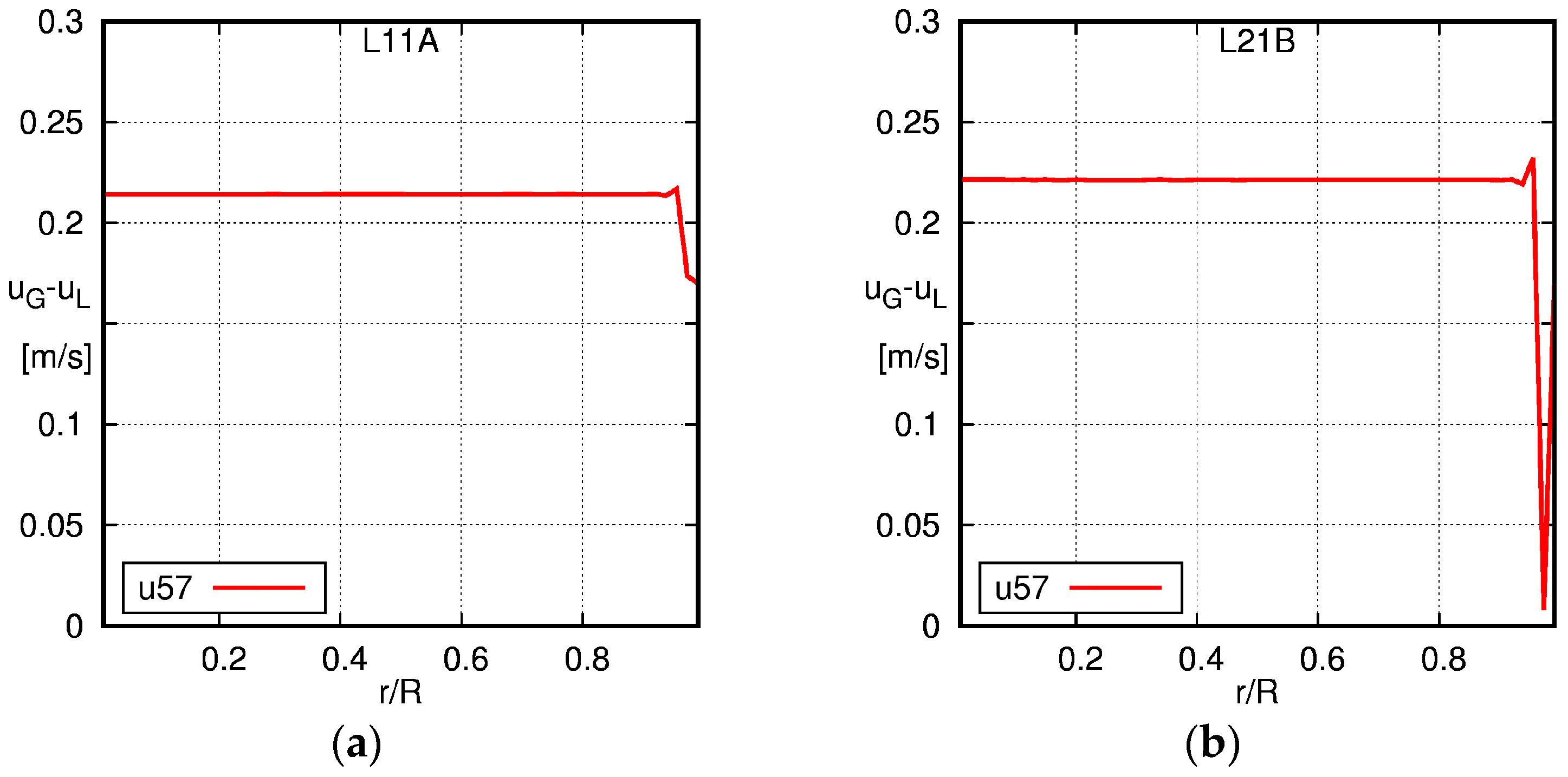
4.1. Pipe with D ≈ 5 cm: Liu [36]

As mentioned before, the results of the simulations of the experiments of Liu [36] have already been presented in our previous paper, and a detailed discussion, as well as single-phase studies concerning the sensitivity to the grid can be found in that paper [32]. Here, we only shortly recapitulate the two-phase flow results for completeness and comparison with the simulation results with different pipe diameters that follow in the next two sections.

In Figure 2, the profiles of the gas fraction are presented, showing, generally speaking, a reasonable agreement between simulation results and experimental data. Larger differences are seen only close to the wall, where a too high gas fraction is obtained from the simulations compared to the experimental data. In the core of the pipe, the computed void matches the experimental data well. Only in case L21C is a core peak seen in the experimental data. As no information on the bubble size distribution is available and only the average diameter has been given by Liu [36], it is not possible to clarify whether this peak is due to large bubbles, which will accumulate in the pipe center.

The profiles of the liquid velocity obtained from the simulations are contrasted with the measurement data of Liu [36] in Figure 3. Overall, a quite good match of both profiles can be seen. For cases L21B and L22A, very similar flat profiles are seen in both experimental data and the simulation result. In cases L11A and L21C, the profiles obtained from the experimental data are less flat across the radius, whereas the simulation results show a flat profile with a steep gradient close to the wall.

The square root of the turbulent kinetic energy computed from the simulations is compared with the measured axial liquid velocity fluctuations in Figure 4. As described in Section 2.1, assuming either isotropic or unidirectional turbulence, an estimate for the upper and lower bounds of the turbulent kinetic energy can be obtained from these fluctuations. These bounds are displayed as error bars in Figure 4.

With the exception of case L21C, too high values for the turbulent kinetic energy are computed in the simulations in the core of the pipe (r < 0.8 R), and the differences are rather large. Slightly smaller differences between the simulation and experiment can observed in the outer part of the pipe.

As only the liquid velocity was measured in Liu [36], only the profiles obtained from the simulations can be shown for the relative velocity. As can be seen in Figure 5, the relative velocity is constant along the diameter of the pipe, except for very close to the wall, where it oscillates. As already discussed in the previous section, these fluctuations are an indicator of the shortcomings of the current modelling approach when the grid size near the walls is smaller than the bubble size.

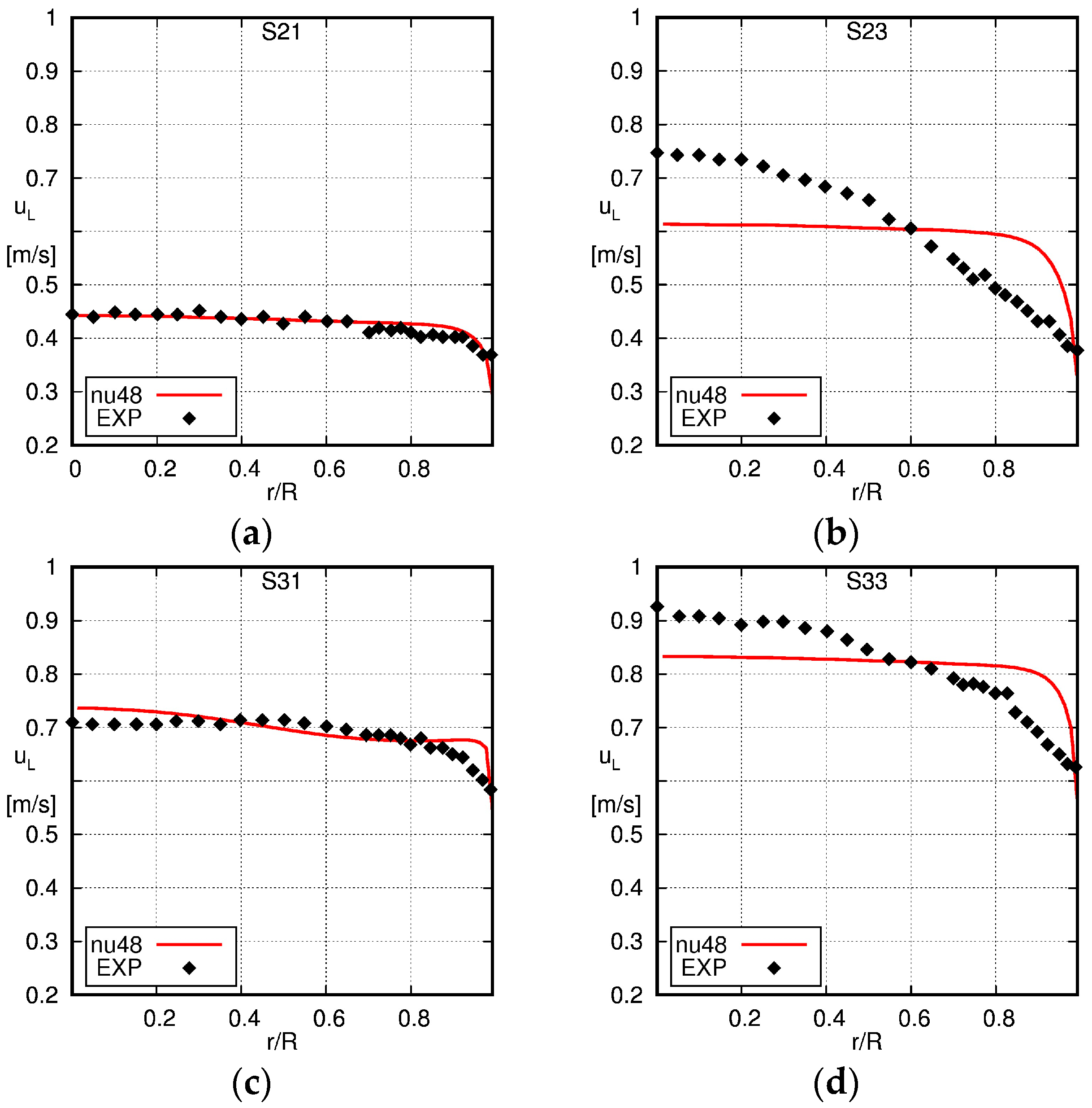
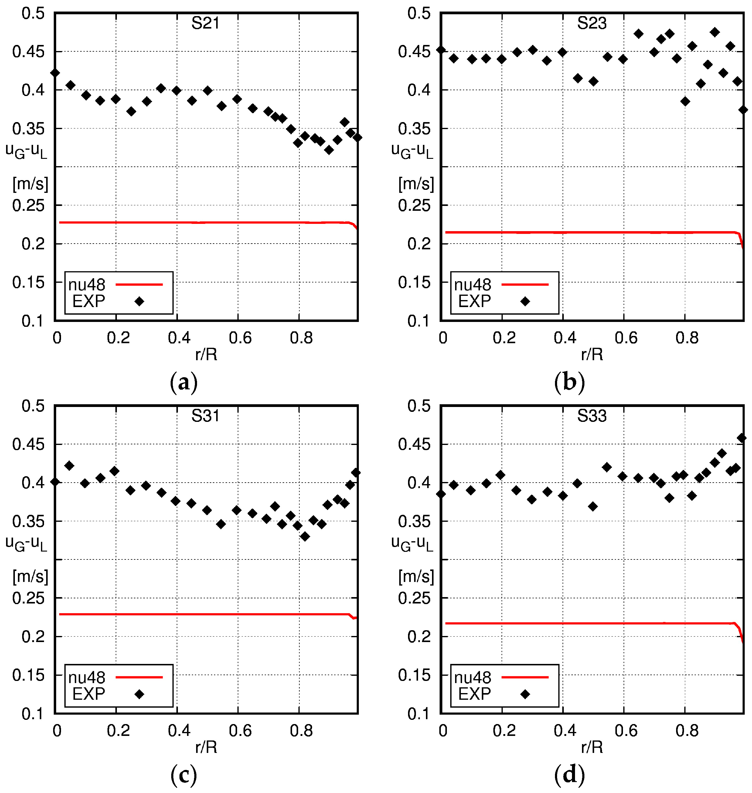
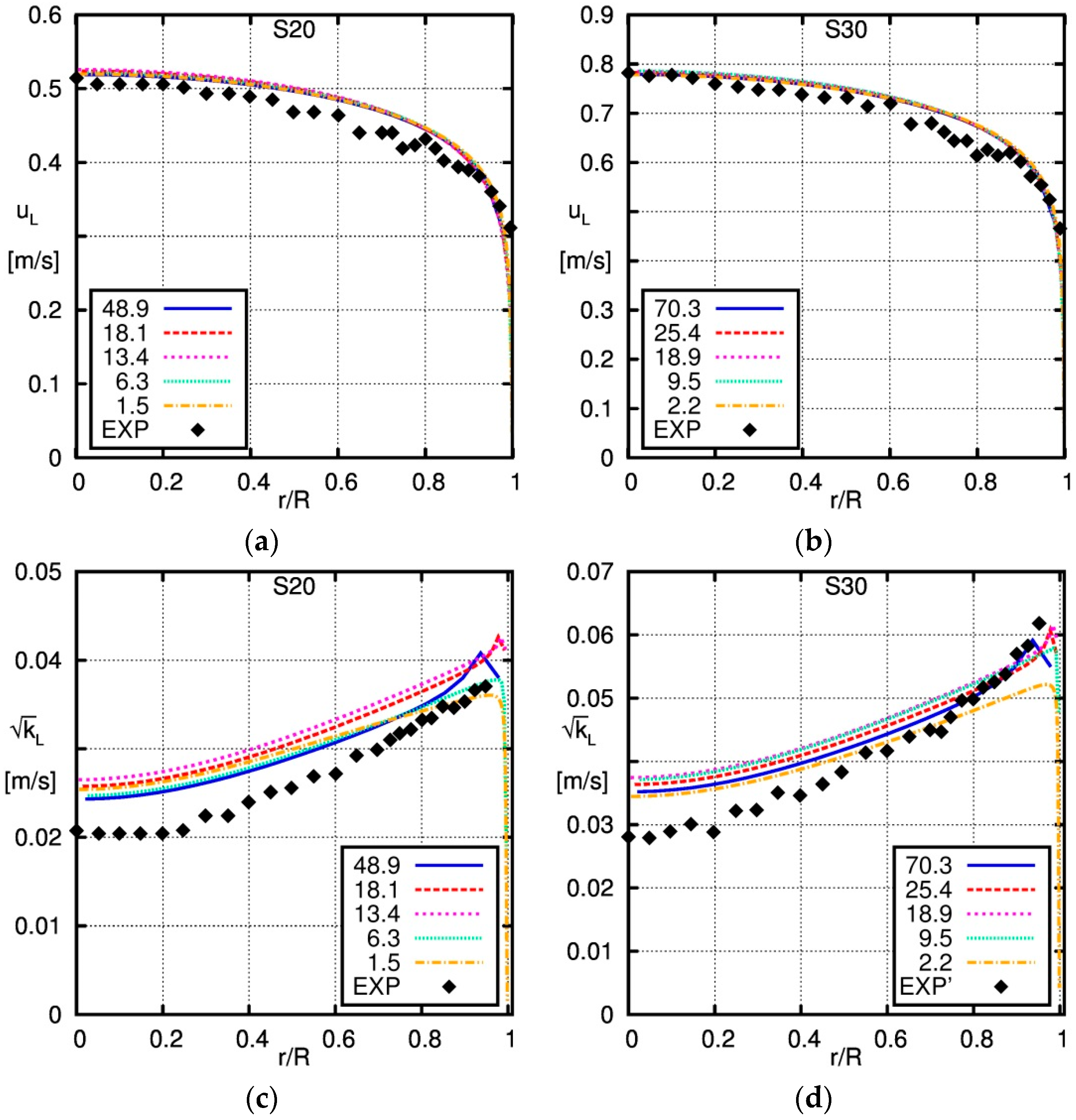
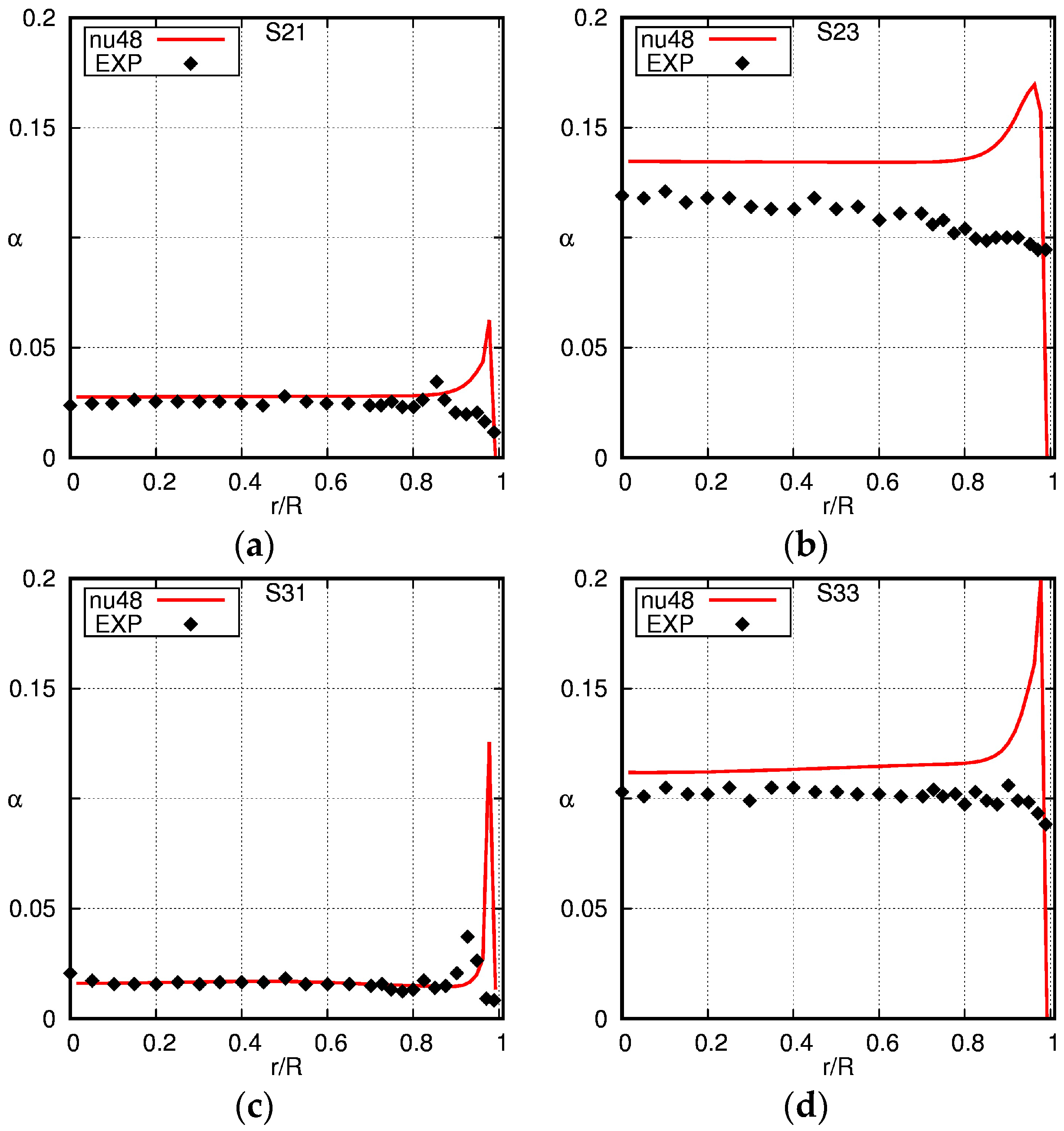
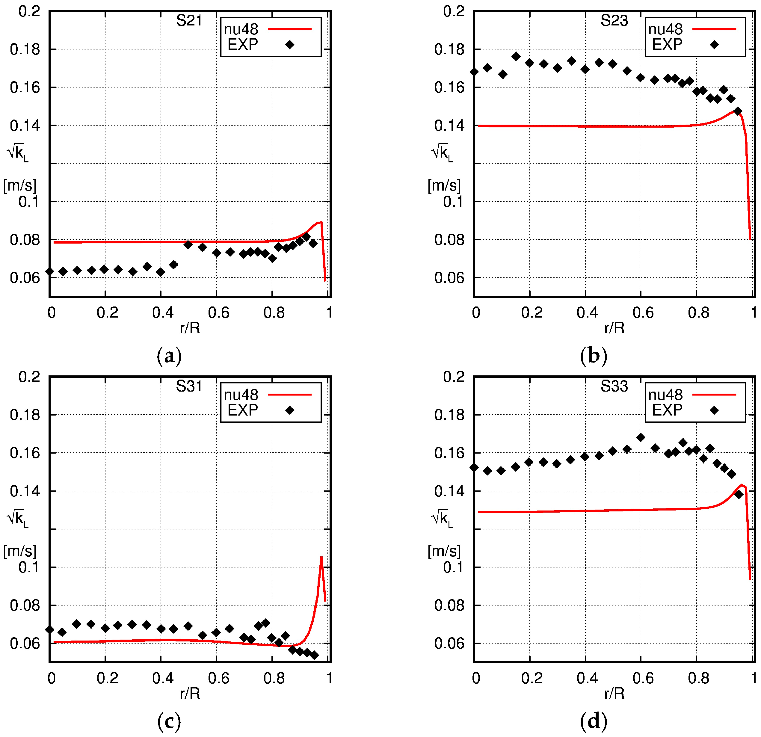
4.2. Pipe with D = 20 cm: Shawkat et al. [33]

4.2.1. Single-Phase Flow

To begin with, results for single-phase flows are compared to the experimental data of Shawkat et al. [33] to study the sensitivity with respect to the grid. Uniform and non-uniform grids where used to compute the flow field, which are given in

Table 3. Different grids used in the simulations of the single-phase pipe flow measured by Shawkat et al. [33].

Grid	nz	nr	$\mathit{\psi }\mathbf{=}\frac{\Delta x_{\mathit{s}\mathit{m}\mathit{a}\mathit{l}\mathit{l}}}{\Delta x_{\mathit{l}\mathit{a}\mathit{r}\mathit{g}\mathit{e}}}$	$\Delta x_{small} \left(mm\right)$	y+
					S20	S30
u24	224	24	1.0	4.167	48.9	70.3
nu48	448	48	0.5	1.443	18.1	25.4
u96	896	96	1.0	1.042	13.4	18.9
nu48	448	48	0.1	0.528	6.3	9.5
nu192	448	192	0.1	0.133	1.5	2.2

. The values of y⁺ of the midpoints of the near-wall cells in the measurement position range between 1.5 and 50 for case S20 (J_L = 0.45 m/s) and between two and 70 for case S30 (J_L = 0.68 m/s).

As shown in Figure 6, the liquid velocity profiles obtained from the simulation on different grids virtually collapse on each other with almost no difference visible. Furthermore, the simulated profiles match the experimentally-measured profiles quite well.

The profiles of the turbulent kinetic energy show some dependency on the grid. However, this dependency is rather irregular with respect to the size of the near-wall cell and is likely to be attributed to the wall function that is used. As pointed out by Kalitzin et al. [51] and Knopp [52], a wall function has to be consistent with the turbulence model in order to be able to achieve grid independency. Consistency in this context means that a fine grid solution of the turbulence model of a zero-pressure gradient boundary layer flow without the use of a wall function should coincide with the analytical value computed from the wall-function model.

This feature is not inherent in most of the commonly-used wall functions, which are available in CFD software packages. Compared to the liquid velocity, larger differences can be observed between the experimentally-obtained profiles for the turbulent kinetic energy and the ones obtained from the simulations. In particular, in the center of the pipe, the turbulent kinetic energy is over-estimated by about 20% to 30%.

4.2.2. Two-Phase Flow

Simulation results obtained for the four selected cases of Shawkat et al. [33] are shown in Figure 7, Figure 8, Figure 9 and Figure 10 and compared against the corresponding experimental data. At the lower gas fluxes (cases S21 and S31), wall-peaked profiles are obtained in the experiments. For these cases, the gas fraction in the core of the pipe is well reproduced by the simulations, as can be seen in Figure 7; however, somewhat larger deviations are found for the location and the height of the wall peak. No wall peak is visible in the experimental data for cases S23 and S33 given in Figure 7; rather, the gas fraction increases slowly, but monotonously towards the center of the pipe. In contrast, a pronounced wall peak is still apparent in the profiles obtained from the simulations. Furthermore, the gas fraction in the pipe center is slightly higher in the simulation results compared to the experimental data.

Liquid velocity profiles are shown in Figure 8. Similar as for the gas fraction profiles, also the profiles of the axial liquid velocity obtained from experiment and simulation match reasonably well for the lower superficial gas velocities. For the higher gas fluxes that were used in cases S23 and S33, larger discrepancies can be observed. Whereas one still finds a flat profile in the pipe core with a steep decrease near the wall in the simulation results, a differently-shaped profile is obtained experimentally showing a decrease of the velocity from the center towards the wall over almost the whole pipe radius. An explanation for the observed differences might be that the average bubble diameter in cases S23 and S33 is larger than in cases S21 and S31. For the former cases, it is about 5 mm, hence in the region where the lift force coefficient strongly decreases and even becomes negative for bubble sizes larger than about 6 mm, according to the correlation of Tomiyama et al. [44]. Unfortunately, also here, no bubble size distribution has been measured; only a radial profile of the average bubble diameter is given. The average diameter increases towards the center of the pipe; hence, it is likely that a size distribution exists, and consequently, the larger bubbles accumulate in the core of the pipe. This in turn leads to a higher liquid velocity in the core of the pipe and, therefore, to a decrease of the velocity towards the wall over the whole pipe radius.

In Figure 9, the profiles of the square root of the turbulent kinetic energy are depicted. Again, quite good agreement of the simulations results with the experimental data is visible for the low gas flux cases S21 and S31. For case S21, some discrepancies show up in the core of the pipe, and for case S31, a too large wall peak in the turbulent kinetic energy is computed with the model.

For cases S23 and S33, somewhat larger differences between the experimental data and the results from the simulations are found: a too low turbulent kinetic energy is computed over the whole radius compared to the experiments. Considering that a two-parameter turbulence model is used, the overall agreement is also quite fair for these two cases and comparable to the agreement in the single-phase case shown in Figure 6.

Furthermore, the bubble velocity was measured by Shawkat et al. [33]; therefore, the radial profiles of the relative velocity are presented in Figure 10. In both the simulation results and experimental data, an almost constant relative velocity over the radius can be seen, although some fluctuations are visible in the experimentally-obtained data.

Strikingly, the relative velocity is higher in the experiments than in the simulations by about a factor of two, which is quite unexpected, in particular in view of the good agreement found for the data of Hosokawa and Tomiyama [34], as will be shown in next section.

Looking for an explanation, one has to note that the relative velocity obtained from the simulations is determined by the model for the drag force that was used. A critical assessment of the drag force model used and the assumptions implied by this model, as well as a short literature overview on the measurements of the relative velocity in bubbly pipe flow will therefore be given in Section 5.

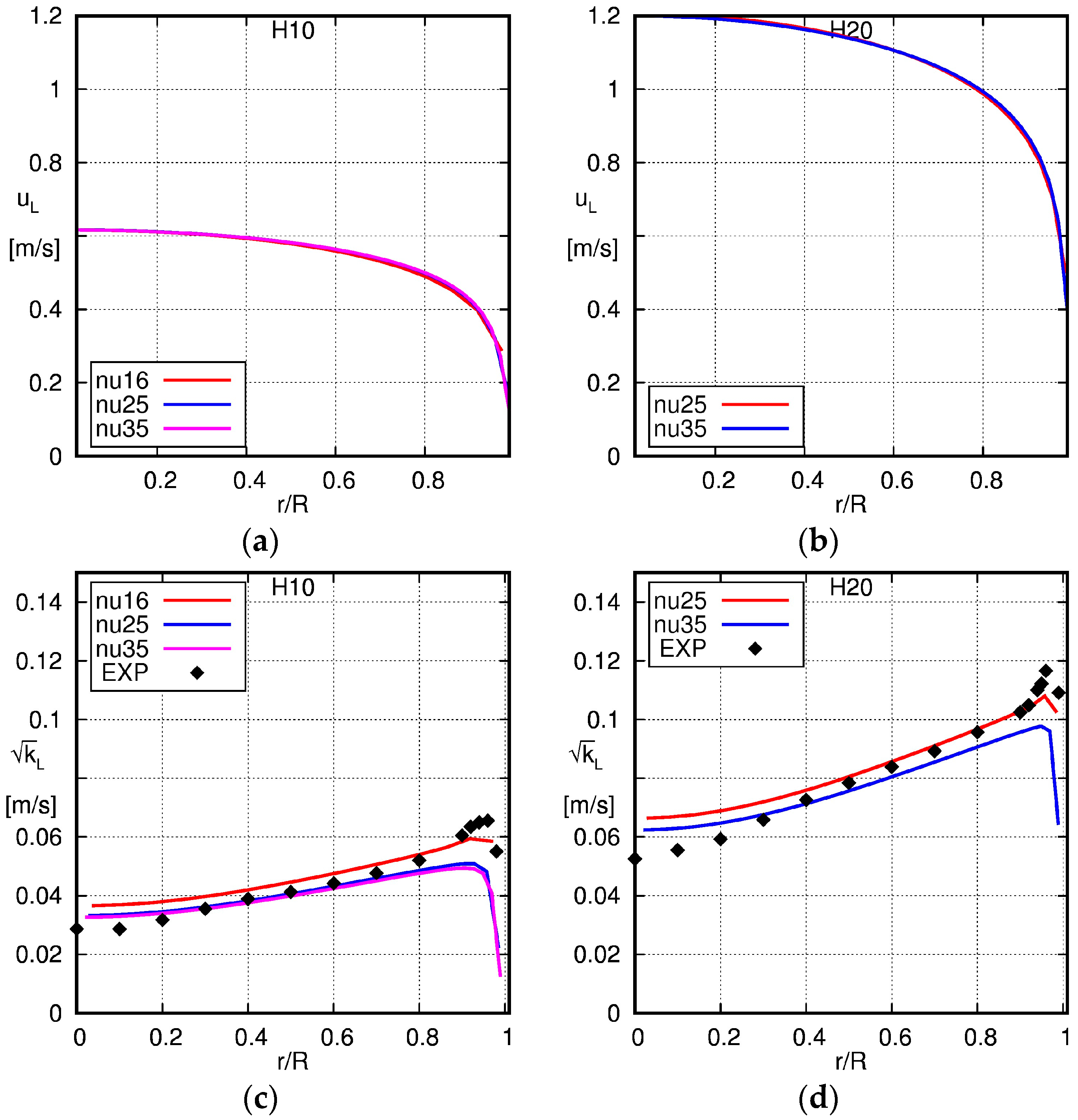
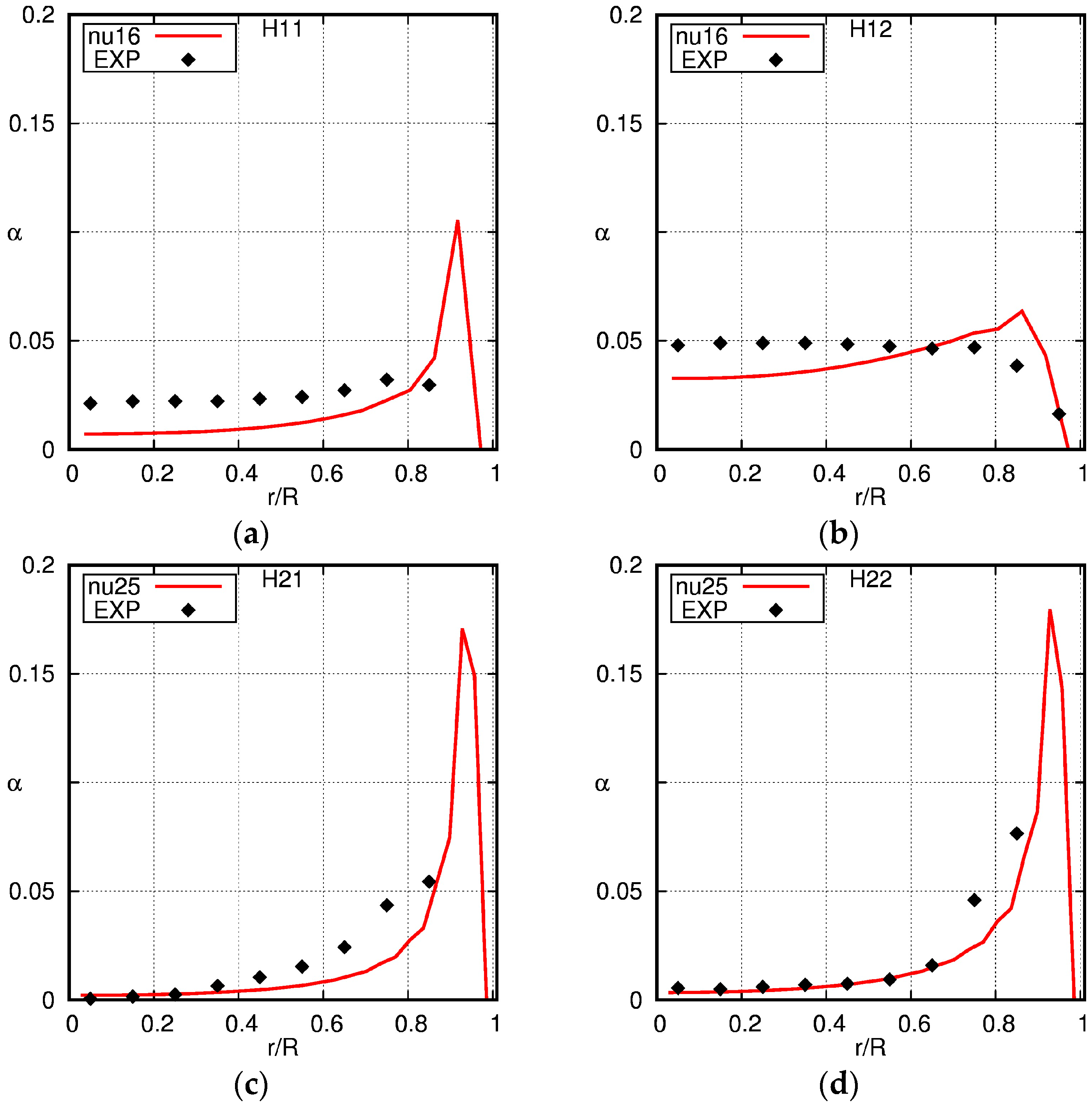
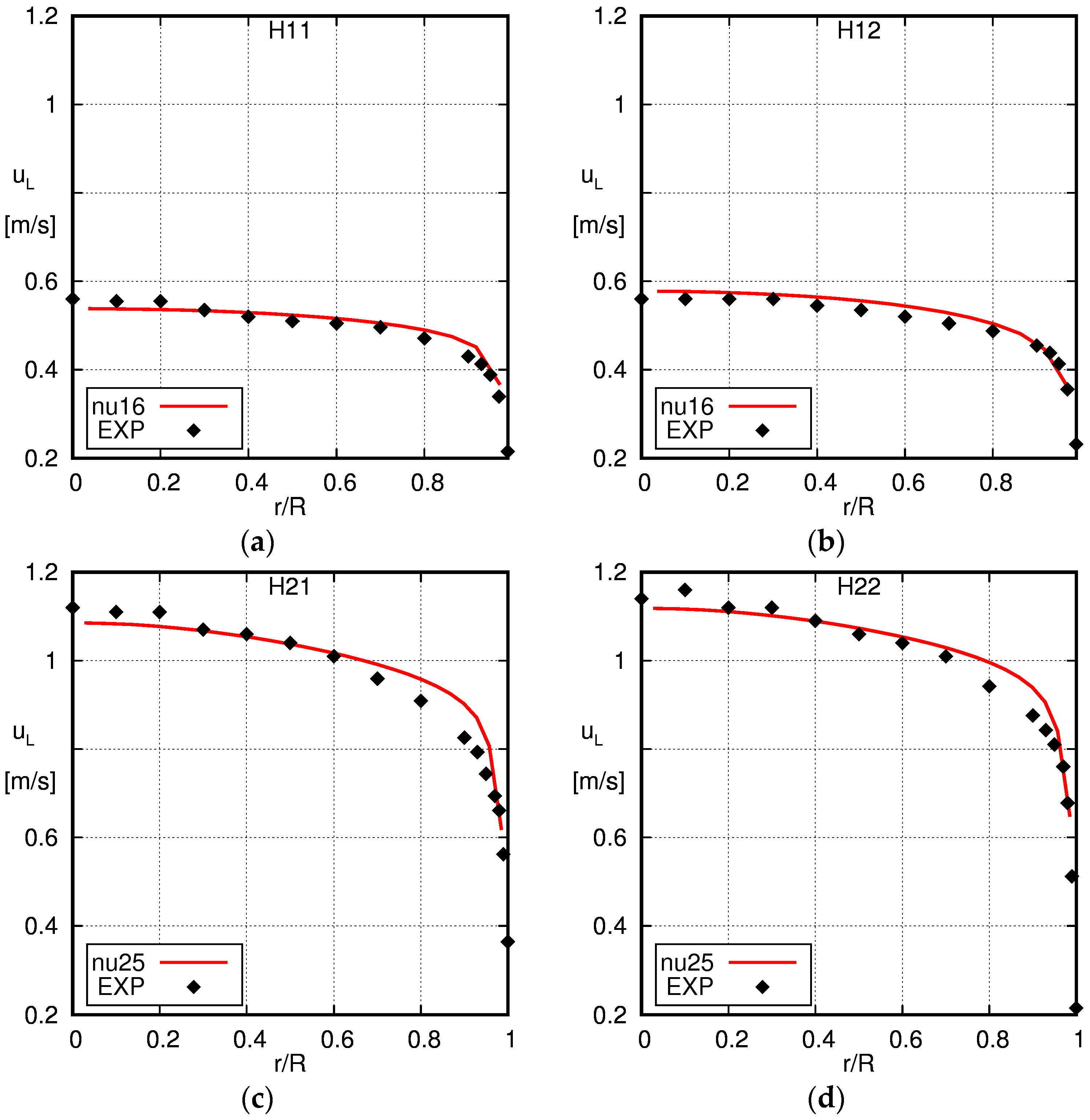
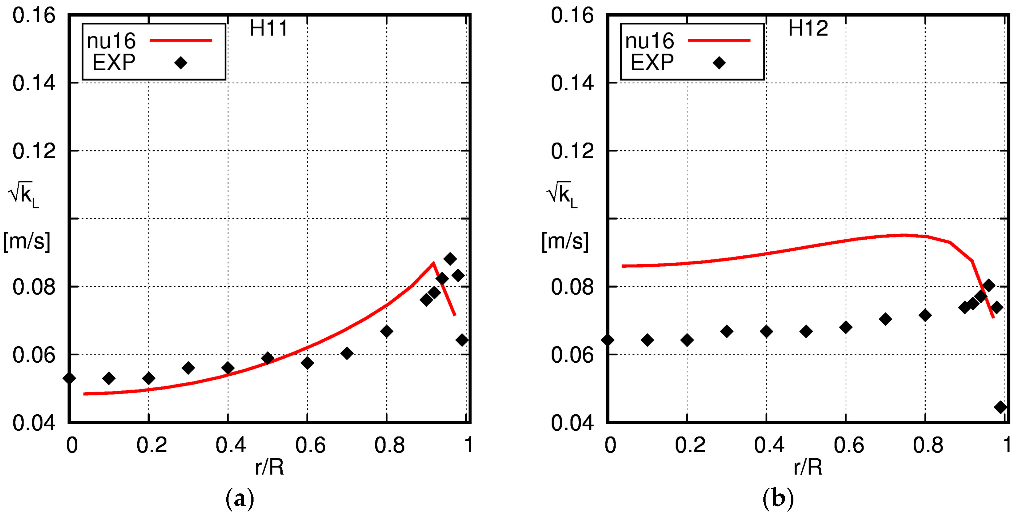
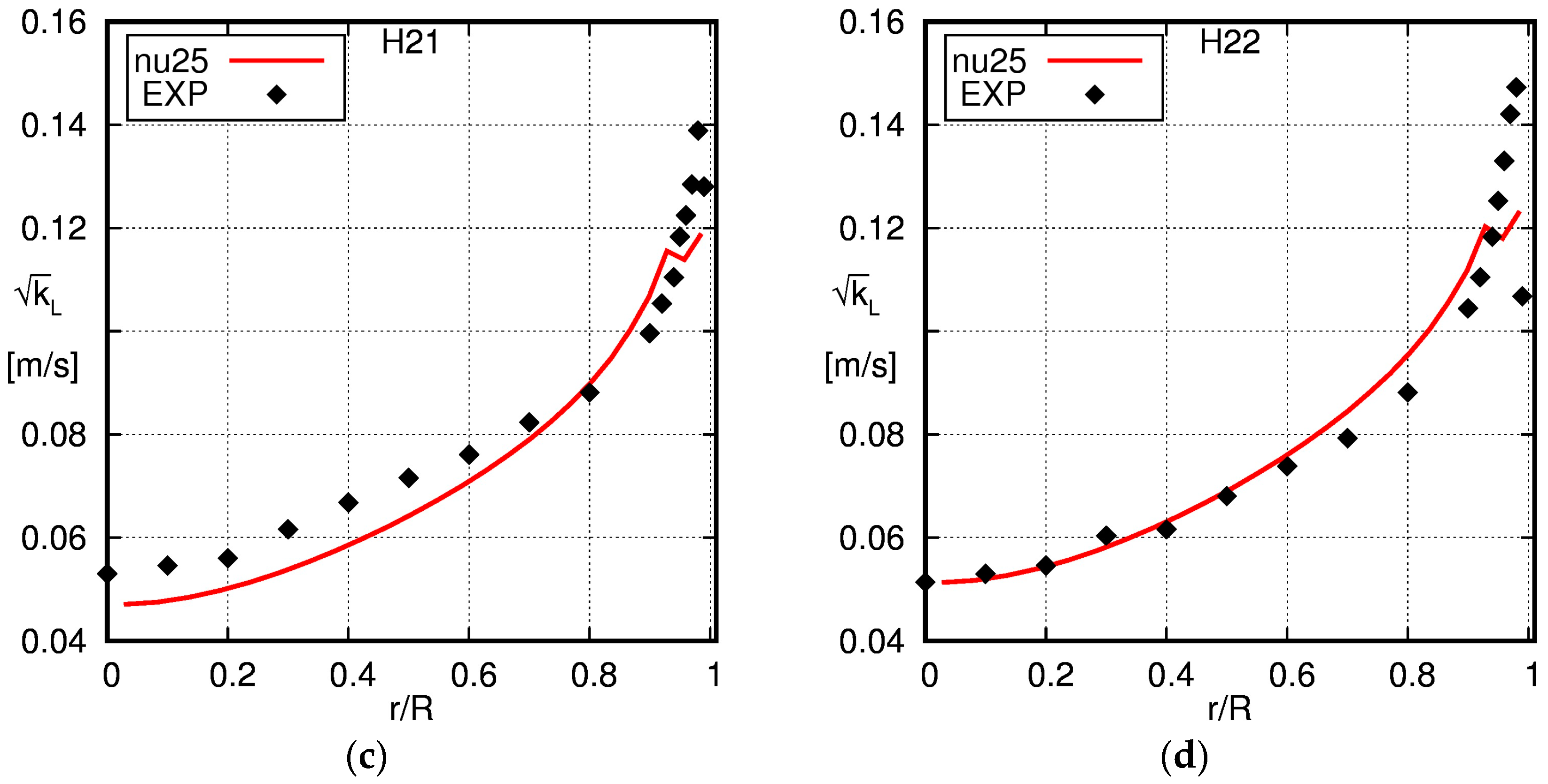
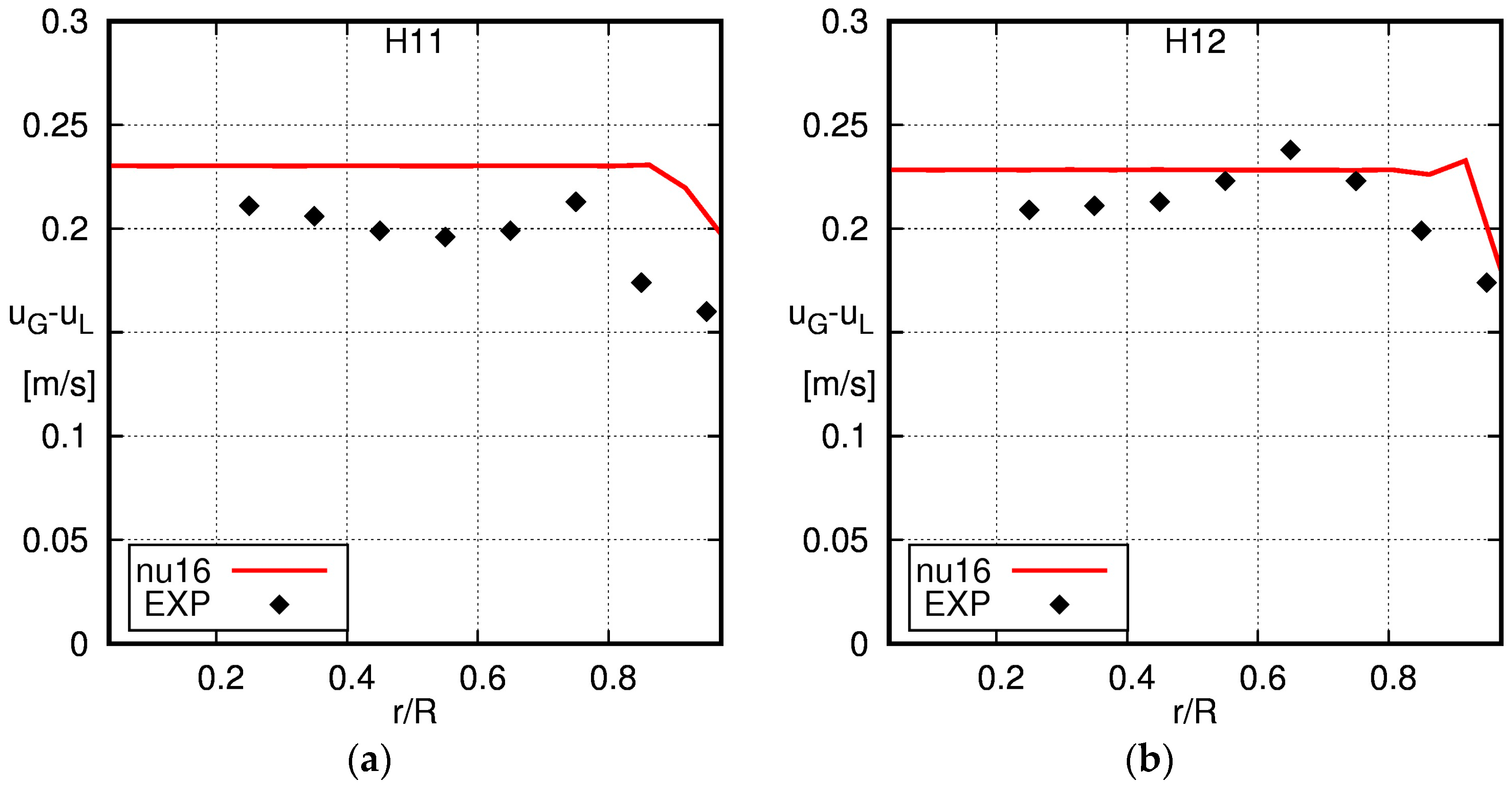
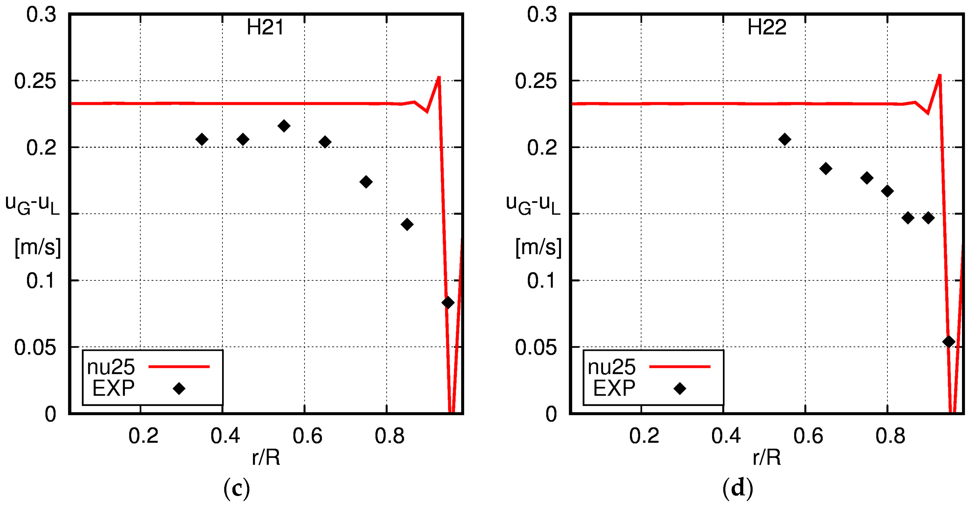
4.3. Pipe with D = 2.5 cm: Hosokawa and Tomiyama [34]

4.3.1. Single-Phase Flow

To begin with, the results for single-phase flows are compared to the experimental data of Hosokawa and Tomiyama [34] to study the sensitivity with respect to the grid. Uniform and non-uniform grids where used to compute the flow field, which are given in

Table 4. Different grids used in the simulations of the single-phase pipe flow measured by Hosokawa and Tomiyama [34].

Grid	nz	nr	$\mathit{\psi }\mathbf{=}\frac{\Delta x_{\mathit{s}\mathit{m}\mathit{a}\mathit{l}\mathit{l}}}{\Delta x_{\mathit{l}\mathit{a}\mathit{r}\mathit{g}\mathit{e}}}$	$\Delta x_{small} \left(mm\right)$	y+
					H10	H20
nu16	399	16	0.75	0.674	12.5	xx
nu25	399	25	0.5	0.346	5.9	11.6
nu35	399	35	0.5	0.247	4.2	7.8

.

The liquid velocity profiles obtained from the simulation on different grids virtually collapse on each other with almost no difference visible. Unfortunately, no measurement data on the average liquid velocity for the single-phase flows are given in Hosokawa and Tomiyama [34], and only the turbulent kinetic energy measurements are provided, which are compared to the simulation results in Figure 11.

The profiles of the turbulent kinetic energy show some dependency on the grid; however, this dependency is to be expected as explained in Section 5. Overall, the agreement of the simulation results and the experimental data for the turbulent kinetic energy is quite satisfactory.

4.3.2. Two-Phase Flow

Experimental data for gas fraction, liquid velocity, turbulent kinetic energy and relative velocity are compared with the simulation results in Figure 12, Figure 13, Figure 14 and Figure 15.

Figure 12 shows the gas fractions for all four cases. Pronounced wall peaks in the gas fraction profiles are observed for liquid superficial velocities of J_L = 1.0 m/s (cases H21 and H22), which are reasonably well reproduced by the simulations. Furthermore, in the bulk of the flow, the gas fraction is reasonably well reproduced by the simulations. For the lower liquid fluxes of J_L = 0.5 m/s (cases H11 and H12), a different picture emerges.

For the lower gas superficial velocity and smaller diameter of the bubbles (case H11), a slight increase of the gas fraction towards the wall can be observed in the experiments. The simulation results show a profile that has a too high peak near the wall and a too low gas fraction in the core of the pipe. For case H12, which has a larger gas flux and larger bubbles, an almost constant gas fraction in the core of the pipe is observed that continuously decreases near the wall, or in other words, a flat profile can be seen, whereas the simulations show a wall-peak in the void-fraction profile. This can, at least partly, be explained by the bubble size distributions given in Hosokawa and Tomiyama [34]. A fraction of the bubbles has a diameter that is larger than 5 mm; hence, these bubbles are already in the region where the lift coefficient steeply drops and turns negative when bubbles are larger than about 6 mm according to the correlation of Tomiyama et al. [44]. In other words, these bubbles will not be pushed towards the wall due to the lift force. Due to the monodisperse approximation, these bubbles are not well represented in the simulations.

Radial profiles of the liquid velocity obtained from our simulations are plotted in Figure 13 together with the experimentally-obtained profiles of Hosokawa and Tomiyama [34], and one finds reasonable agreement for all cases. Somewhat flatter profiles are obtained from the simulations, in particular for the higher liquid velocity flux of J_L = 1.0 m/s, which results in a steeper decrease near the wall and a lower velocity in the center of the pipe.

The experimentally-obtained profiles of the turbulent kinetic energy shown in Figure 14 match the simulation results quite well, with the exception of case H12. Whereas larger differences occur only near the wall for cases H11, H21 and H22, the turbulent kinetic energy obtained from the simulation is too high by about 50% compared to the experiments for case H12.

The relative velocity is depicted in Figure 15. In the center region, a constant relative velocity is found in the experimental data and the simulation data; however, the simulation results for the relative velocity are slightly higher than the experimentally-obtained values. This deviation is considered insignificant given the accuracy of the drag force correlation by Ishii and Zuber [43]. For a more detailed discussion, see Section 5. The relative velocity decreases with decreasing wall distance in the experimental data for r/R larger than about 0.6–0.8. According to Hosokawa and Tomiyama [34], this can be attributed to the higher aspect ratio of the bubbles near the wall, which leads to an increased drag, hence to a reduced relative velocity. This effect is not included in the current drag model and, therefore, is not captured in the simulations, where the relative velocity is constant up to the wall. In the first three cells, the relative velocity shows some oscillations, which is due to the limitations of the model, when the near-wall cells are smaller than the bubbles, and shows the need for improved near-wall modelling.

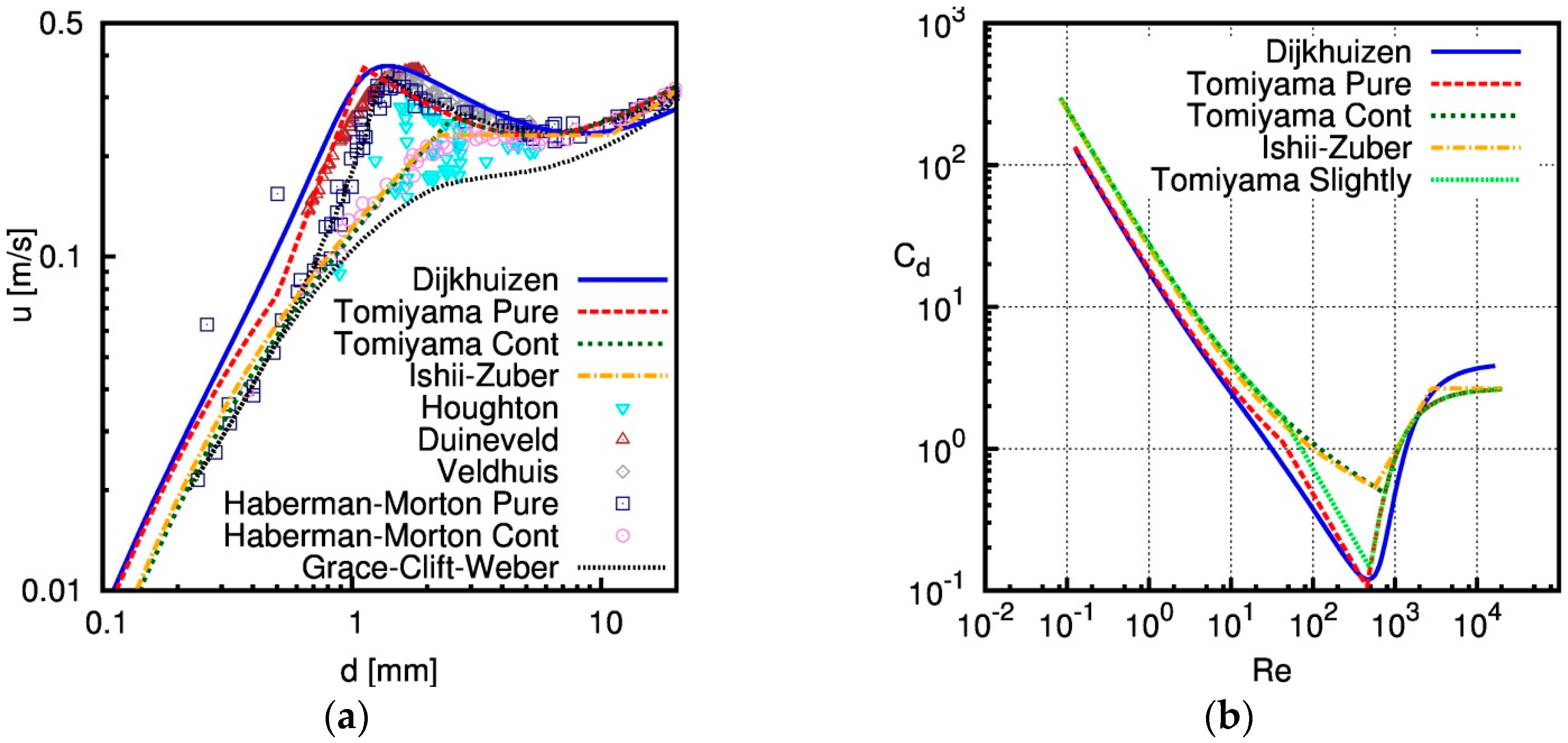
5. Models and Data for Drag Force and Rise Velocity

The unexpected deviations between calculated and measured relative bubble velocities in the experiments of Shawkat et al. [33], shown in Figure 10, call for an investigation of possible causes. To this end, we first summarize in the following the effects neglected in the present modelling of the drag force and estimate the consequences on the predictions. Since it turns out that in all cases, a reduction of rise velocity would be expected rather than the observed increase, we then review other sources of data on relative bubble velocities and the used measurement methods in order to estimate possible errors in the data.

5.1. Critical Assessment of the Drag Force Modelling

Here, the correlation proposed by Ishii and Zuber [43] for bubbles rising in an infinite, quiescent liquid is used. One can think of several factors, which might have an influence on the actual drag force:

• the “degree of contamination” of the water in air-water flows.
• the influence of pipe walls and shear rate.
• the influence of background turbulence.
• the influence of higher gas fractions (swarm effects).

It is long known that for air bubbles in water, the terminal velocity, and hence, also the drag force, depends on the degree of contamination of the water [53], but the actual degree of contamination is often difficult to quantify. The drag force correlation of Ishii and Zuber [44] is valid for “contaminated” water, which gives a higher drag and, hence, a lower rise velocity than correlations that are valid for “pure” water, such as the ones proposed by Tomiyama et al. [54] or Dijkhuizen et al. [55]. The drag coefficient computed for air-bubbles rising in water is shown on the right in Figure 16 as a function of the terminal Reynolds number. The corresponding computed terminal rise velocity is shown on the left of Figure 16. In addition, experimentally-determined rise velocities for air bubbles in ultra-purified water (Duineveld [56] and Veldhuis [57]), for air bubbles in filtered or distilled and in tap water (Haberman and Morton [58]) and for air bubbles in sea water (Houghton et al. [59]) are shown in that figure, as well as the bounds for pure and contaminated water proposed by Clift et al. [53] in Figure 7.3 of their famous book.

The rise velocity computed using the drag coefficient proposed by Ishii and Zuber [43] indeed nicely follows the experimental data for tap water given by Haberman and Morton [58], which is also well reproduced using the correlation given by Tomiyama et al. [54] for contaminated water. Interestingly, the rise velocity of air bubbles in contaminated water that was given by Clift et al. [53] is lower than the experimental data of Haberman and Morton [58] and also than the values computed using the correlations of Ishii and Zuber [43] or by Tomiyama et al. [54] for bubble diameters in the range of 1 mm to about 10 mm. Only some of the experimental data by Houghton et al. [59] obtained for air bubbles in sea water are somewhat closer to the values by Clift et al. [53].

Differences between the measurement data of the rise velocity obtained with tap water and those obtained with purified water are only visible for bubbles with a diameter smaller than about 4 mm. The rise velocity of purified water increases with decreasing diameter and reaches a maximum of about 0.36 m/s for a bubble diameter of about 1.5 to 2.0 mm. Subsequently, the rise velocity decreases again with decreasing diameter. A different “state of purification” of the water is evidently important for the rise velocity of bubbles smaller than about 1 mm. Here, differences in the measured rise velocity can be observed for the ultra-purified water used by Duineveld [56] and the measured data for filtered water of Haberman and Morton [58].

To summarize, one sees that for a bubble diameter of about 4.5 mm, which was measured in the experiments of Shakwat [4], the differences in the rise velocity obtained with the different correlations for the drag coefficient are rather small, 0.231 m/s for Ishii–Zuber, 0.233 m/s for Tomiyama and 0.256 m/s for Dijkhuizen, and do not explain the observed differences between simulation and experiments in Figure 10. Indeed, in additional simulations using the correlations by Tomiyama et al. [54] and Dijkhuizen et al. [55], only minor differences could be observed in the results.

The effect of pipe walls and shear rate would be to increase the drag force and, hence, reduce the slip velocity of the phases as discussed by Hososkawa and Tomiyama [34]. Furthermore, high shear rates occur only in a region near the wall; hence, this effect would be localized in a region near the wall. This is consistent with the differences observed in our simulation results with the experimental data of Hosokawa and Tomiyama [34], but offers no explanation for the differences observed here.

No clear picture concerning the effect of background turbulence in the liquid phase has emerged yet. The literature that is available, however, suggests that the drag coefficient should rather increase, which means the rise velocity will decrease (see, for example, Okawa et al. [60], Ghatage et al. [61]).

Quite a bit of research has been done on how swarm effects at a higher gas fraction influence the drag force, respectively rise velocity (e.g., Simonnet et al. [62] and Roghair et al. [63]). However, from the data available, one finds that for the diameter and gas fraction obtained in the experiments of Shawkat et al. [33], swarm effects tend to increase the drag only slightly and, therefore, still can be neglected.

5.2. Review of Further Measurements of Bubble Rise Velocity

Unfortunately, the literature on experiments with turbulent bubbly pipe flows, in which the velocities of both phases have been measured, is limited. The following overview serves to get an idea about possible measurement inaccuracies as the cause of the deviations.

In their pioneering works, Serizawa et al. [64,65,66,67] describe measurements of air-water bubbly flow in a pipe of 60 mm in diameter using a dual needle resistivity probe and hot film anemometry. The liquid superficial velocity was varied between 0.44 m/s and 1.03 m/s, and the gas superficial velocity was varied between 0 m/s and 0.4 m/s. The measured mean bubble diameter was 3.5 to 4 mm in all of the experiments, and the relative velocity varied between 0.15 and 0.38 m/s.

Liu and Bankoff [68,69] report experiments on turbulent air-water flows in a pipe with a diameter of 38 mm. The measurements were also performed with dual needle resistivity probes and hot film anemometers. The gas flux was varied between J_G = 0.027 m/s and J_G = 0.347 m/s and the liquid flux between J_L = 0.376 m/s and J_L = 1.391 m/s. The measured bubble size was in the range of 2 mm to 4 mm. The relative velocity was found to vary between 0.1 and 0.4 m/s, depending on the radial position and the gas and liquid superficial velocities.

Samstag [70] has measured bubbly air-water flows in a 70 mm diameter pipe using a dual sensor resistivity probe and an x-wire hot film probe. For a liquid superficial velocity of J_L = 1.44 m/s and gas superficial velocities of J_G = 0.076 m/s and J_G = 0.16 m/s, he found relative velocities in the range of 0.15 to 0.25 m/s. Under the assumption of a spherical shape, he computed a mean bubble diameter in the range d_B = 3 mm to d_B = 4 mm from the chord lengths that were measured.

Mudde and Saito [71] have measured bubbly flow of air and water in a 149-mm pipe with superficial velocities of J_L = 0.175 m/s and J_G = 0.0366 m/s using a four-point optical probe and laser Doppler anemometry. The mean bubble diameter was also in the range of 3 to 4 mm, and the relative velocity varied between 0.21 and 0.27 m/s along the radius of the pipe.

Fujiwara et al. [72] used a projected shadow image technique and particle-image-velocimetry/laser-induced-fluorescence (PIV/LIF) to measure gas and liquid phase properties in turbulent bubbly flow in a pipe of a 44-mm diameter at a water superficial velocity of J_L = 0.22 m/s and two different air superficial velocities of J_G = 0.0024 m/s and J_G = 0.0049 m/s. The average bubble diameter was 2 mm, and the slip velocity between the phases was in the range of 0.19 m/s to 0.25 m/s.

Colin et al. [73] measured air-water two-phase flow in a pipe of a 40-mm diameter. They determined the gas and liquid phase properties using a dual fiber optical probe and a hot wire anemometer at liquid superficial velocities in the range of 0.23 m/s to 1 m/s and gas superficial velocities between 0.023 m/s and 0.046 m/s. The average bubble diameter was found to be 3.3 to 3.5 mm, and the relative velocity was about 0.25 to 0.27 m/s in the center of the pipe and decreased towards the wall.

From the foregoing overview, it becomes clear that also other experimental data that are available in literature exhibit significant variations in the relative velocity of the bubbles under similar conditions. Concerning different measurement techniques that have been used in the investigations, a certain trend emerges. The early works of Seriwaza et al. [64,65,66], Liu and Bankoff [68,69] and Samstag [70], which are based on dual needle resistivity probes, show a particularly wide spread in the relative velocity depending on the flow conditions. The later works, such as Mudde and Saito [71], Fujiwara et al. [72] and Colin et al. [73], which employ optical probes or photographic techniques, rather support our expectations that the slip velocity should be close to the terminal velocity of a single bubble rising in an infinite quiescent medium.

6. Discussion and Conclusions

In the present work, a baseline model that has been defined for monodisperse adiabatic bubbly flow has been applied to simulate co-current upward flow in pipes of different diameters. Three different experimental datasets available from the literature have been chosen, which have comparable liquid and gas phase properties, but differ in the diameter of the pipe. Overall, the differences observed between the experimental data and the simulation results are comparable for the different diameter pipes, and the experimental data are satisfactorily reproduced by the simulations.

For all three datasets, the simulations show a wall-peaked profile of the gas fraction for all combinations of gas and liquid superficial velocities, whereas core-peaked profiles are observed in some of the experiments, e.g., case H12 of Hosokawa and Tomiyama [34] and S23 and S33 of Shawkat et al. [33]. However, also for those experimental data that show a wall peak, differences in the location of the wall peak can be observed, and the height of the peak is overestimated in the simulation results. The shape of the radial profile of the gas fraction is mainly determined by the non-drag forces, that means lift, wall and turbulent dispersion force. Compared to the large number of works concerning the modelling of the drag force, as presented in Section 5, considerably fewer studies are concerned with the non-drag forces. Hence, a much larger uncertainty concerning their modelling prevails and is discussed controversially, as presented, e.g., in [74]. Especially the lift coefficient is often tuned for the specific experimental data that one tries to simulate (e.g., [75,76]). In line with our baseline strategy, we have used a fixed set of closures, and no case to case tuning is done. The too high peaks in the gas fraction can be explained by the too large lift resulting from the steep velocity gradients next to the wall. Therefore, the modelling of near-wall effects is a promising candidate to obtain a better match between the profiles obtained from experiment and simulation.

The liquid velocity profiles that were measured are well represented by the simulation data for all experiments with the notable exception of cases S23 and S33 of Shawkat et al. [33]. In those two cases, an almost constant velocity is computed in the core of the pipe (r/R < 0.9) with a strong decrease close to the wall, whereas the experiments show a continuous decrease over almost the whole radius.

The differences in turbulent kinetic energy estimated from the experimental data and computed in the simulations are surprisingly small considering the many open questions still related to turbulence in multiphase flows. No clear trend is visible in the differences between experiments and simulation: a close match, over-prediction and under-prediction by the simulations are seen. Clearly, more work is necessary on the understanding and modelling of bubble-induced turbulence, and also, more complex turbulence models, such as Reynolds stress models, should be tried. Of course, in order to validate more complex turbulence models, reliable measurement data of the Reynolds stresses in two-phase flows are necessary.

Some surprising observations were made for those experiments in which both gas and liquid phase velocity were measured. The slip velocity between the phases provided by Hosokawa and Tomiyama [34] matches well with the expectation that the Ishii–Zuber closure for the drag provides a reasonable estimate for the drag coefficient for the cases considered in this work. Compared to those experiments, a too high slip velocity near the walls is obtained from the simulations, which can be explained by the effects of confining pipe walls. However, compared to the data given by Shawkat et al. [33], the slip velocity in our simulation results is consistently lower, almost by a factor of two. Neither the effects of walls, mean shear flow, background turbulence or hindered rise due to the presence of other bubbles offer an explanation of this discrepancy. A review of further literature that provided measurements of both liquid and gas phase velocities in bubbly two-phase flows showed that the data of some more recent works [71,72,73] using optical probes or photographic techniques are consistent with the Ishii–Zuber closure, whereas earlier measurement data [64,65,66,68,69,70] employing dual needle resistivity probes show a wide spread in the relative velocity of both phases.

Unfortunately, despite the extensive considerations in Section 5, no definitive explanation of the observed differences can be given, and one can only speculate. While it seems unlikely that the drag correlation by itself is the cause of the discrepancies, it could be that also some larger bubbles were present in the experiments of Shawkat et al. [33], which would lead to a cooperative rise and, hence, a higher relative velocity of the phases. In this case, modelling those experiments as monodisperse bubbly flow would not suffice. However, model validation would then require measurements on the bubble size distribution, which are not available for these tests. Alternatively, the data on the bubble velocities might be susceptible to some systematic measurement error, which is hard to pin down.

Nevertheless, the following conclusions can be drawn:

• The baseline model reproduces the experimental data reasonably well independent of the pipe diameter.
• Further improvements of the baseline model are desirable, in particular for the near-wall modelling and the closure for bubble-induced turbulence.

Moreover, a few desiderata concerning data for model validation should be emphasized, which are essential for further progress in the field of Euler-Euler modelling of bubbly flows and are often not satisfied by the presently-available results. These might be considered “general wisdom”, but the discussion of Section 5, made in an attempt to explain the differences in the relative velocity observed in some of the present results, highlights their importance:

• Knowledge of the full bubble size distribution is essential to explain the observed behavior in bubbly flows. Hence, data including measurements of bubble size distributions are necessary. In addition, such data would also allow a validation of models for bubble coalescence and breakup, as described, e.g., in [77].
• Generally, validation of CFD models for bubbly flow requires more reliable measurement techniques. In particular, reliable measurements of the bubble and liquid velocity are surprisingly scarce at present.
• It is highly desirable that experimental databases for CFD validation provide a comprehensive set of measurements, including both gas and liquid phase properties. At least bubble diameter, liquid and gas velocity profiles and profiles for the liquid turbulent kinetic energy should be given. Otherwise, important features may be missed by the validation.
• Considering the sensitivity of the air-water system to even the smallest contaminations, which are hard to avoid and even harder to quantify, measurement data of other less sensitive systems of gas and liquid should be acquired.

References

1. Marschall, H.; Mornhinweg, R.; Kossmann, A.; Oberhauser, S.; Langbein, K.; Hinrichsen, O. Numerical simulation of dispersed gas/liquid flows in bubble-columns at high phase fractions using OpenFOAM® part 1—Modeling fundamentals. Chem. Eng. Technol. 2010, 82, 2129–2140. [Google Scholar]
2. Jakobsen, H.A.; Lindborg, H.; Dorao, C.A. Modeling of bubble-column reactors: Progress and limitations. Ind. Eng. Chem. Res. 2005, 44, 5107–5151. [Google Scholar] [CrossRef]
3. Sokolichin, A.; Eigenberger, G.; Lapin, A. Simulation of buoyancy driven bubbly flow: Established simplifications and open questions. AIChE J. 2004, 50, 24–45. [Google Scholar] [CrossRef]
4. Podowski, M. On the consistency of mechanistic multidimensional modeling of gas/liquid two-phase flows. Nucl. Eng. Des. 2009, 239, 933–940. [Google Scholar] [CrossRef]
5. Serizawa, A.; Tomiyama, A. Some remarks on mechanisms of phase distribution in an adiabatic bubbly pipe flow. Multiph. Sci. Technol. 2003, 15, 79–98. [Google Scholar] [CrossRef]
6. Masood, R.; Delgado, A. Numerical investigation of the interphase forces and turbulence closure in 3D square bubble columns. Chem. Eng. Sci. 2014, 108, 154–168. [Google Scholar] [CrossRef]
7. Silva, M.K.; d’Avila, M.A.; Mori, M. Study of the interfacial forces and turbulence models in a bubble column. Comput. Chem. Eng. 2012, 44, 34–44. [Google Scholar] [CrossRef]
8. Diaz, M.E.; Montes, F.J.; Galan, M.A. Influence of the lift force closures on the numerical simulation of bubble plumes in a rectangular bubble column. Chem. Eng. Sci. 2009, 64, 930–944. [Google Scholar] [CrossRef]
9. Hibiki, T.; Ishii, M. Lift force in bubbly flow systems. Chem. Eng. Sci. 2007, 62, 6457–6474. [Google Scholar] [CrossRef]
10. Selma, B.; Bannari, R.; Proulx, P. A full integration of a dispersion and interface closures in the standard k-epsilon model of turbulence. Chem. Eng. Sci. 2010, 65, 5417–5428. [Google Scholar] [CrossRef]
11. Ekambara, K.; Dhotre, M. CFD simulation of bubble column. Nucl. Eng. Des. 2010, 240, 963–969. [Google Scholar] [CrossRef]
12. Tabib, M.V.; Roy, A.R.; Joshi, J.B. CFD simulation of bubble column—An analysis of interphase forces and turbulence models. Chem. Eng. J. 2008, 139, 589–614. [Google Scholar] [CrossRef]
13. Zhang, D.; Deen, N.G.; Kuipers, J.A.M. Numerical simulation of the dynamic flow behavior in a bubble column: A study of closures for turbulence and interface forces. Chem. Eng. Sci. 2006, 61, 7593–7608. [Google Scholar] [CrossRef]
14. Politano, M.; Carrica, P.; Converti, J. A model for turbulent polydisperse two-phase flow in vertical channels. Int. J. Multiph. Flow 2003, 29, 1153–1182. [Google Scholar] [CrossRef]
15. Troshko, A.A.; Hassan, Y.A. A Two-equation turbulence model of turbulent bubbly flows. Int. J. Multiph. Flow 2001, 27, 1965–2000. [Google Scholar] [CrossRef]
16. Morel, C. Turbulence modeling and first numerical simulations in turbulent two-phase flows. In Proceedings of the Eleventh Symposium on Turbulent Shear Flows, Grenoble, France, 8–10 September 1997.
17. Buffo, A.; Marchisio, D.L. Modeling and simulation of turbulent polydisperse gas-liquid systems via the generalized population balance equation. Rev. Chem. Eng. 2014, 30, 73–126. [Google Scholar] [CrossRef]
18. Selma, B.; Bannari, R.; Proulx, P. Simulation of bubbly flows: Comparison between direct quadrature method of moments (DQMOM) and method of classes (CM). Chem. Eng. Sci. 2010, 65, 1925–1941. [Google Scholar] [CrossRef]
19. Fox, R.O. Introduction and fundamentals of modeling approaches for polydisperse multiphase flows. In Multiphase Reacting Flows: Modelling and Simulation; Marchisio, D.L., Fox, R.O., Eds.; Springer-Verlag: Vienna, Austria, 2007. [Google Scholar]
20. Sanyal, J.; Marchisio, D.L.; Fox, R.O.; Dhanasekharan, K. On the comparison between population balance models for CFD simulation of bubble columns. Ind. Eng. Chem. Res. 2005, 44, 5063–5072. [Google Scholar] [CrossRef]
21. Sattar, M.A.; Naser, J.; Brooks, G. Numerical simulation of two-phase flow with bubble break-up and coalescence coupled with population balance modeling. Chem. Eng. Process. 2013, 70, 66–76. [Google Scholar] [CrossRef]
22. Chen, P.; Sanyal, J.; Dudukovic, M. Numerical simulation of bubble columns flows: Effect of different breakup and coalescence closures. Chem. Eng. Sci. 2005, 60, 1085–1101. [Google Scholar] [CrossRef]
23. Wang, T.; Wang, J.; Jin, Y. Population balance model for gas-liquid flows: Influence of bubble coalescence and breakup models. Ind. Eng. Chem. Res. 2005, 44, 7540–7549. [Google Scholar] [CrossRef]
24. Sarhan, A.R.; Naser, J.; Brooks, G. CFD simulation on influence of suspended solid particles on bubbles’ coalescence rate in flotation cell. Int. J. Miner. Process. 2016, 146, 54–64. [Google Scholar] [CrossRef]
25. Li, W.; Zhong, W. CFD simulation of hydrodynamics of gas-liquid-solid three-phase bubble column. Powder Technol. 2015, 286, 766–788. [Google Scholar] [CrossRef]
26. Ojima, S.; Sasaki, S.; Hayashi, K.; Tomiyama, A. Effects of particle diameter on bubble coalescence in a slurry bubble column. J. Chem. Eng. Jpn. 2015, 48, 181–189. [Google Scholar] [CrossRef]
27. Rzehak, R.; Krepper, E. Closure models for turbulent bubbly flows: A CFD study. Nucl. Eng. Des. 2013, 265, 701–711. [Google Scholar] [CrossRef]
28. Rzehak, R.; Krepper, E. Bubbly flows with fixed polydispersity: Validation of a baseline closure model. Nucl. Eng. Des. 2015, 287, 108–118. [Google Scholar] [CrossRef]
29. Rzehak, R.; Krepper, E.; Liao, Y.; Ziegenhein, T.; Kriebitzsch, S.; Lucas, D. Baseline Model for Simulation of Bubbly Flows. Chem. Eng. Technol. 2015, 38, 1972–1978. [Google Scholar] [CrossRef]
30. Ziegenhein, T.; Lucas, D.; Rzehak, R.; Krepper, E. Closure relations for CFD simulation of bubble columns. In Proceedings of the 8th International Conference on Multiphase Flow (ICMF 2013), Jeju, Korea, 26–31 June 2013.
31. Ziegenhein, T.; Rzehak, R.; Lucas, D. Transient simulation for large scale flow in bubble columns. Chem. Eng. Sci. 2015, 122, 1–13. [Google Scholar] [CrossRef]
32. Rzehak, R.; Kriebitzsch, S.H.L. Multiphase CFD-simulation of bubbly pipe flow: A code comparison. Int. J. Multiph. Flow 2015, 68, 135–152. [Google Scholar] [CrossRef]
33. Shawkat, M.; Ching, C.; Shoukri, M. Bubble and liquid turbulence characteristics of bubbly flow in a large diameter vertical pipe. Int. J. Multiph. Flow 2008, 34, 767–785. [Google Scholar] [CrossRef]
34. Hosokawa, S.; Tomiyama, A. Multi-fluid simulation of turbulent bubbly pipe flows. Chem. Eng. Sci. 2009, 64, 5308–5318. [Google Scholar] [CrossRef]
35. Rzehak, R.; Krepper, E. CFD modeling of bubble-induced turbulence. Int. J. Multiph. Flow 2013, 55, 138–155. [Google Scholar] [CrossRef]
36. Liu, T.J. The role of bubble size on liquid phase turbulent structure in two-phase bubbly flow. In Proceedings of the 3rd International Conference on Multiphase Flow (ICMF’98), Lyon, France, 8–12 June 1998.
37. Michiyoshi, I.; Serizawa, A. Turbulence in two-phase bubbly flow. Nucl. Eng. Des. 1986, 95, 253–267. [Google Scholar] [CrossRef]
38. Wang, S.K.; Lee, S.J.; Jones, O.C., Jr.; Lahey, R.T., Jr. 3-D turbulence structure and phase distribution measurements in bubbly two-phase flows. Int. J. Multiph. Flow 1987, 13, 327–343. [Google Scholar] [CrossRef]
39. Drew, D.A.; Passman, S.L. Theory of Multicomponent Fluids; Springer-Verlag: New York, NY, USA, 1998. [Google Scholar]
40. Yeoh, G.H.; Tu, J.Y. Computational Techniques for Multiphase Flows—Basics and Applications; Butterworth-Heinemann: Oxford, UK, 2010. [Google Scholar]
41. Ishii, M.; Hibiki, T. Thermo-Fluid Dynamics of Two-Phase Flow, 2nd ed.; Springer-Verlag: New York, NY, USA, 2011. [Google Scholar]
42. Rzehak, R.; Ziegenhein, T.; Kriebitzsch, S.; Krepper, E.; Lucas, D. Unified modeling of bubbly flows in pipes, bubble columns, and airlift columns. Chem. Eng. Sci. 2016, in press. [Google Scholar] [CrossRef]
43. Ishii, M.; Zuber, N. Drag coefficient and relative velocity in bubbly, droplet or particulate flows. AIChE J. 1979, 25, 843–855. [Google Scholar] [CrossRef]
44. Tomiyama, A.; Tamai, H.; Zun, I.; Hosokawa, S. Transverse migration of single bubbles in simple shear flows. Chem. Eng. Sci. 2002, 57, 1849–1858. [Google Scholar] [CrossRef]
45. Hosokawa, S.; Tomiyama, A.; Misaki, S.; Hamada, T. Lateral migration of single bubbles due to the presence of wall. In Proceedings of the ASME Joint U.S.-European Fluids Engineering Division Conference (FEDSM 2002), Montreal, QC, Canada, 14–18 July 2002.
46. Rzehak, R.; Krepper, E.; Lifante, C. Comparative study of wall-force models for the simulation of bubbly flows. Nucl. Eng. Des. 2012, 252, 41–49. [Google Scholar] [CrossRef]
47. Burns, A.D.; Frank, T.; Hamill, I.; Shi, J.-M. The Favre averaged drag model for turbulence dispersion in Eulerian multi-phase flows. In Proceedings of the 5th International Conference on Multiphase Flow (ICMF 2004), Yokohama, Japan, 30 May–4 June 2004.
48. Sankaranarayanan, K.; Shan, X.; Kevrekidis, I.G.; Sundaresan, S. Analysis of drag and virtual mass forces in bubbly suspensions using an implicit formulation of the lattice Boltzmann method. J. Fluid Mech. 2002, 452, 61–96. [Google Scholar] [CrossRef]
49. Menter, F.R. Review of the shear-stress transport turbulence model experience from an industrial perspective. Int. J. Comput. Fluid Dyn. 2009, 23, 305–316. [Google Scholar] [CrossRef]
50. OpenCFD. OpenFOAM User Guide v2.2.2; OpenFOAM Foundation: London, UK, 2013. [Google Scholar]
51. Kalitzin, G.; Medic, G.; Iaccarino, G.; Durbin, P. Near-wall behavior of RANS turbulence models and implications for wall functions. J. Comput. Phys. 2005, 204, 265–291. [Google Scholar] [CrossRef]
52. Knopp, T. Model-consistent universal wall-functions for RANS turbulence modelling. In Proceedings of the International Conference on Boundary and Interior Layers (BAIL 2006), Göttingen, Germany, 24–28 July 2006.
53. Clift, R.; Grace, J.R.; Weber, M.E. Bubbles, Drops and Particles; Acadamic Press: New York, NY, USA, 1978. [Google Scholar]
54. Tomiyama, A.; Kataoka, I.; Zun, I.; Sakaguchi, T. Drag coefficients of single bubbles under normal and micro gravity conditions. JSME Int. J. Ser. B 1998, 41, 472–479. [Google Scholar] [CrossRef]
55. Dijkhuizen, W.; Roghair, I.; van Sint Annaland, M.; Kuipers, J.A.M. DNS of gas bubbles behaviour using an improved 3D front tracking model—Drag force on isolated bubbles and comparison with experiments. Chem. Eng. Sci. 2010, 65, 1415–1426. [Google Scholar] [CrossRef]
56. Duineveld, P.C. The rise velocity and shape of bubbles in pure water at high Reynolds number. J. Fluid Mech. 1995, 292, 325–332. [Google Scholar] [CrossRef]
57. Veldhuis, C. Leonardo’s Paradox: Path and Shape Instabilities of Particles and Bubbles. Ph.D. Thesis, University of Twente, Enschede, The Netherlands, 7 February 2007. [Google Scholar]
58. Haberman, W.; Morton, R. An Experimental Investigation of the Drag and Shape of Air Bubbles Rising in Various Liquids; Report 802; The David W. Taylor Model Basin: Washington, DC, USA, 1953. [Google Scholar]
59. Houghton, G.; Ritchie, P.; Thomson, J. Velocity of rise of air bubbles in sea-water, and their types of motion. Chem. Eng. Sci. 1957, 7, 111–112. [Google Scholar] [CrossRef]
60. Okawa, T.; Torimoto, K.; Nishiura, M.; Kataoka, I.; Mori, M. Effects of turbulence and containing wall on rise velocities of single bubbles in a vertical circular pipe. In Proceedings of the 10th International Conference on Nuclear Engineering (ICONE10), Arlington, VA, USA, 14–18 April 2002.
61. Ghatage, S.V.; Sathe, M.J.; Doroodchi, E.; Joshi, J.B.; Evans, G.M. Effect of turbulence on particle and bubble slip velocity. Chem. Eng. Sci. 2013, 100, 120–136. [Google Scholar] [CrossRef]
62. Simonnet, M.; Gentric, C.; Olmos, E.; Midoux, N. Experimental determination of the drag coefficient in a swarm of bubbles. Chem. Eng. Sci. 2007, 62, 858–866. [Google Scholar] [CrossRef]
63. Roghair, I.; van Sint Annaland, M.; Kuipers, J.A.M. Drag force and clustering in bubble swarms. AIChE J. 2013, 59, 1791–1800. [Google Scholar] [CrossRef]
64. Serizawa, A.; Kataoka, I.; Michiyoshi, I. Turbulence structure of air-water bubbly flow—I. Measuring techniques. Int. J. Multiph. Flow 1975, 2, 221–233. [Google Scholar] [CrossRef]
65. Serizawa, A.; Kataoka, I.; Michiyoshi, I. Turbulence structure of air-water bubbly flow—II. Local properties. Int. J. Multiph. Flow 1975, 2, 235–246. [Google Scholar] [CrossRef]
66. Serizawa, A.; Kataoka, I.; Michiyoshi, I. Turbulence structure of air-water bubbly flow—III. Transport properties. Int. J. Multiph. Flow 1975, 2, 247–259. [Google Scholar] [CrossRef]
67. Serizawa, A.; Kataoka, I.; Michiyoshi, I. Experimental data set No. 24: Phase distribution in bubbly flow. Multiph. Sci. Technol. 1992, 6, 257–301. [Google Scholar] [CrossRef]
68. Liu, T.; Bankoff, S. Structure of air–water bubbly flow in a vertical pipe. I: Liquid mean velocity and turbulence measurements. Int. J. Heat Mass Transf. 1993, 36, 1049–1060. [Google Scholar] [CrossRef]
69. Liu, T.; Bankoff, S. Structure of air–water bubbly flow in a vertical pipe. II: Gas fraction, bubble velocity and bubble size distribution. Int. J. Heat Mass Transf. 1993, 36, 1061–1072. [Google Scholar] [CrossRef]
70. Samstag, M. Experimentelle Untersuchungen von Transportphänomenen in Vertikalen Turbulenten Luft-Wasser-Blasenströmungen. Ph.D. Thesis, University Karlsruhe, Karlsruhe, Germany, 1996. [Google Scholar]
71. Mudde, R.F.; Saito, T. Hydrodynamical similarities between bubble column and bubbly pipe flow. J. Fluid Mech. 2001, 437, 203–228. [Google Scholar] [CrossRef]
72. Fujiwara, A.; Minato, D.; Hishida, K. Effect of bubble diameter on modification of turbulence in an upward pipe flow. Int. J. Heat Fluid Flow 2004, 25, 481–488. [Google Scholar] [CrossRef]
73. Colin, C.; Fabre, J.; Kamp, A. Turbulent bubbly flow in pipe under gravity and microgravity conditions. J. Fluid Mech. 2012, 711, 469–515. [Google Scholar] [CrossRef] [Green Version]
74. Ziegenhein, T.; Rzehak, R.; Krepper, E.; Lucas, D. Numerical simulation of polydispersed flow in bubble columns with the inhomogeneous multi-size-group model. Chem. Ing. Tech. 2013, 85, 1080–1091. [Google Scholar] [CrossRef]
75. Colombo, M.; Fairweather, M. Multiphase turbulence in bubbly flows: RANS simulations. Int. J. Multiph. Flow. 2015, 77, 222–243. [Google Scholar] [CrossRef]
76. Ekambara, K.; Sean Sanders, R.; Nandakumar, K.; Masliyah, J.H. CFD Modeling of gas-liquid bubbly flow in horizontal pipes: Influence of bubble-coalescence and breakup. Int. J. Chem. Eng. 2012, 2012, 620643:1–620643:20. [Google Scholar] [CrossRef]
77. Liao, Y.; Rzehak, R.; Lucas, D.; Krepper, E. Baseline closure model for dispersed bubbly flow: Bubble-coalescence and breakup. Chem. Eng. Sci. 2015, 122, 336–349. [Google Scholar] [CrossRef]
Figure 1. Investigated geometry of all three cases. As indicated by the gray shaded area, axisymmetrical simulations are performed, and only a thin wedge of the pipe has been modelled.
Fluids 01 00029 g001
Figure 2. Comparison of the radial profiles of the gas fraction obtained using the baseline model with the experimental data of Liu [36]. The solid line is the simulation result and the squares the experimental data (EXP). (a) L11A; (b) L21B; (c) L22A; (d) L21C.
Fluids 01 00029 g002
Figure 3. Comparison of the radial profiles of the liquid velocity obtained using the baseline model with the experimental data of Liu [36]. The solid line is the simulation result and the squares the experimental data (EXP). (a) L11A; (b) L21B; (c) L22A; (d) L21C.
Fluids 01 00029 g003
Figure 4. Comparison of the radial profiles of the turbulent kinetic energy obtained using the baseline model in OpenFOAM with the experimental data of Liu [36]. The solid line is the simulation result and the squares the experimental data (EXP). Note that only the axial liquid velocity fluctuations have been measured in the experiments; therefore, the error bars are given to denote the upper and lower limit of the turbulent kinetic energy based on the assumption of isotropic and unidirectional turbulence, respectively. (a) L11A; (b) L21B; (c) L22A; (d) L21C.
Fluids 01 00029 g004
Figure 5. Radial profiles of the relative velocity obtained using the baseline model. The solid line is the simulation result and the squares the experimental data (EXP). (a) L11A; (b) L21B; (c) L22A; (d) L21C.
Fluids 01 00029 g005aFluids 01 00029 g005b
Figure 6. Comparison of the results obtained for single-phase flow on different grids with experimental data given by Shawkat [33]. S20: JL = 0.45 m/s, S30: JL = 0.68 m/s. The different lines correspond to the y+ values given in Table 3. The squares (EXP) are the experimental data. (a) S20 liquid velocity; (b) S30 liquid velocity; (c) S20 turbulent kinetic energy; (d) S30 turbulent kinetic energy.
Fluids 01 00029 g006
Figure 7. Comparison of the radial profiles of the gas fraction obtained using the baseline model with the experimental data of Shawkat et al. [33]. The solid line is the simulation result and the squares the experimental data (EXP). (a) S21; (b) S23; (c) S31; (d) S33.
Fluids 01 00029 g007
Figure 8. Comparison of the radial profiles of the liquid velocity obtained using the baseline model with the experimental data of Shawkat et al. [33]. The solid line is the simulation result and the squares the experimental data (EXP). (a) S21; (b) S23; (c) S31; (d) S33.
Fluids 01 00029 g008
Figure 9. Comparison of the radial profiles of the turbulent kinetic energy obtained using the baseline with the experimental data of Shawkat et al. [33]. The solid line is the simulation result and the squares the experimental data (EXP). (a) S21; (b) S23; (c) S31; (d) S33.
Fluids 01 00029 g009
Figure 10. Radial profiles of the relative velocity obtained using the baseline with the experimental data of Shawkat et al. [33]. The solid line is the simulation result and the squares the experimental data (EXP). (a) S21; (b) S23; (c) S31; (d) S33.
Fluids 01 00029 g010
Figure 11. Comparison of results obtained for single-phase flow on different grids with experimental data given by Hosokawa and Tomiyama [34]. The solid lines are simulation results and the squares denote experimental data (EXP). H10: JL = 0.5 m/s, H20: JL = 1.0 m/s. (a) H10 liquid velocity; (b) H20 liquid velocity; (c) H10 turbulent kinetic energy; (d) H20 turbulent kinetic energy.
Fluids 01 00029 g011
Figure 12. Comparison of the radial profiles of the gas fraction obtained using the baseline model with the experimental data of Hosokawa and Tomiyama [34]. The solid line is the simulation result and the squares the experimental data (EXP). (a) H11; (b) H12; (c) H21; (d) H22.
Fluids 01 00029 g012
Figure 13. Comparison of the radial profiles of the liquid velocity obtained using the baseline model with the experimental data of Hosokawa and Tomiyama [34]. The solid line is the simulation result and the squares the experimental data (EXP). (a) H11; (b) H12; (c) H21; (d) H22.
Fluids 01 00029 g013
Figure 14. Comparison of the radial profiles of the turbulent kinetic energy obtained using the baseline model with the experimental data of Hosokawa and Tomiyama [34]. The solid line is the simulation result and the squares the experimental data (EXP). (a) H11; (b) H12; (c) H21; (d) H22.
Fluids 01 00029 g014aFluids 01 00029 g014b
Figure 15. Radial profiles of the relative velocity obtained using the baseline model with the experimental data of Hosokawa and Tomiyama [34]. The solid line is the simulation result and the squares the experimental data (EXP). (a) H11; (b) H12; (c) H21; (d) H22.
Fluids 01 00029 g015aFluids 01 00029 g015b
Figure 16. Terminal rise velocity u (a) and drag coefficient CD (b) of single air bubbles rising in quiescent water with different “degrees” of contamination. See the text in Section 5 for a detailed explanation of the sources for the different data (symbols) and correlations (lines).
Fluids 01 00029 g016