
Nonlinear Convection in a Partitioned Porous Layer


Department of Mechanical Engineering, University of Bath, Bath BA2 7AY, UK
Fluids 2016, 1(3), 24; https://doi.org/10.3390/fluids1030024
Submission received: 23 June 2016
/
Revised: 27 July 2016
/
Accepted: 28 July 2016
/
Published: 23 August 2016
(This article belongs to the Special Issue Computational Fluid Dynamics)
Abstract
:Convection in a partitioned porous layer is considered where the thin partition causes a mechanical isolation of the two identical sublayers from one another, but heat may neveretheless conduct freely. An unsteady solver that employs the multigrid method is employed to determine steady-state strongly nonlinear for values of the Darcy–Rayleigh number up to eight times its critical value. The predictions of linear stability theory are confirmed and the accuracy of the computations are carefully monitored and controlled. It is found that the wavenumber for which the maximum rate of heat transfer is attained at any chosen value of the Darcy–Rayleigh number, increases quite strongly from roughly at onset to when . It is also found that convection generally cannot take place with wavenumbers which are close to the left-hand branch of the neutral stability curve because nonlinear interactions favour modes selected from higher harmonics.
1. Introduction
Many authors have studied the effect of different types of layering on the convective instability caused by heating a layer of fluid-saturated porous media from below. The earliest studies begin with those of Georgitzha [1], who considered two cases: a two-layer system with slightly different permeabilities, and one with a weakly spatially varying permeability. Masuoka et al. [2] computed convection patterns in a two-layer system, and Rana, Horne and Cheng [3] modelled convection in three-layer system that represented the Pahoa reservoir in Hawaii. A much more systematc approach was then taken by McKibbin and O’Sullivan [4,5] who considered both the linearized theory and a two-dimensional weakly nonlinear theory. Of interest is the fact that, with two sublayers, it is possible to determine parameter ranges (i.e., of relative permeabilities and sublayer thicknesses) for which the neutral stability curve has two minima, rather than having the more usual unimodal form. Rees and Riley [6] revisited the weakly nonlinear theory in order to determine conditions on those parameters for which two-dimensional rolls do not form the preferred convection pattern, but where cells with square planform appear instead.
Other types of layering involve the sandwiching of the porous layer with solid but heat-conducting layers both above and below. The analysis of Mojtabi and Rees [7], who considered identical solid bounding layers, found that the onset criterion then depends very strongly indeed on the nature of the solid layers. At one extreme, the composite layer mimics well the classical Darcy–Bénard problem by having the critical Darcy–Rayleigh number, and a critical wavenumber, ; in general, this arises when the solid layers are relatively highly conducting. At the other extreme, the layer corresponds to and —this tends to happen when the solid layers are relatively poor conductors of heat (see, for example, the work of Falsaperla et al. [8] who consider the combined effect of rotation and Robin boundary conditions). Other examples of this type of work include the weakly nonlinear analyses of Riahi [9] and Rees and Mojtabi [10], the combined effect of conducting boundaries and a horizontal pressure gradient [11], nonlinear computations [12], and internal conducting layers [13,14,15,16].
Of more relevance to the present work are the analyses of Genç and Rees [17] and Rees and Genç [18]. The former paper considers a porous medium with two identical sublayers that are mechanically isolated from one another by a thin impermeable interface, where independent pressure gradients are applied to the two sublayers. The latter considers a system of N identical sublayers again with thin impermeable interfaces, but now considered as a free convective linear stability analysis. It was found that the large-N limit yields a critical Darcy–Rayleigh number and wavenumber which are more usually associated with the constant-heat-flux variant of the single-layer Darcy–Bénard problem, namely that and . A weakly nonlinear analysis by Rees et al. [19] shows that convection is always two-dimensional immediately post-onset. In the present paper, we consider the two-sublayer case but extend the analysis of Rees and Genç [18] to strongly nonlinear convection using numerical methods. Our aim here, therefore, is to determine the flow and temperature fields and to determine those wavenumbers that maximise the rate of heat transfer as a function of the Darcy–Rayleigh number.
2. Governing Equations
We consider convection in a porous layer which is heated from below and which is split into two identical sublayers by the presence of an impermeable, infinitesimally thin and perfectly heat conducting interface; see Figure 1. The height of the layer is and therefore the sublayers each have height, L. The porous medium is isotropic and otherwise homogeneous with pemeability, K, and the dynamic viscosity of the fluid is μ. The lower surface of the layer is held at the uniform temperature, , while the upper surface is held at where . We define a reference temperature drop according to
and this represents the temperature drop across one of the two sublayers.
We shall confine our attention to two-dimensional flow only; this is not a restriction for moderate values of the Darcy–Rayleigh number because the weakly nonlinear analysis of Rees et al. [19] shows that the preferred convection pattern in the postcritical range is expected to be two-dimensional at first. On taking the velocity field to be , the conservation of mass yields:
and Darcy’s law, subject to the Boussinesq approximation, takes the form
The equation governing the transport of heat is given by
The upper and lower surfaces together with the interface are impermeable and, therefore, we need to apply
At the interface, , the continuity of both the temperature and the heat flux (i.e., temperature gradient) needs to be imposed.
The equations and boundary conditions are rendered dimensionless using the following transformations:
and then the governing equations become
and
Given that the flow is two-dimensional, we may define the streamfunction, ψ, using
which means that Equation (8) is satisfied automatically. Thus the elimination of p between Equations (9) and (10) means that the nondimensional governing equations for the porous medium and the boundary conditions become
In the above the Darcy–Rayleigh number is given by
and it is therefore based upon the height and the mean temperature drop across one sublayer. This convention was introduced in Genç and Rees [17] and Rees and Genç [18] in order to be able to compare critical values of easily between the single-layer classical Darcy–Bénard problem and cases where there are any number of sublayers stacked above one another. Should one require a Darcy–Rayleigh number which is based upon the thickness and the temperature drop across the whole of the layer, rather than one sublayer, then it will be precisely .
3. Numerical Method
Equations (13) and (14) were approximated using a second order accurate finite difference discretisation on a uniform grid. In general, only one convection cell in the horizontal direction was computed, and therefore the boundary conditions given in Equation (15) were supplemented by the following sidewall conditions:
which are exactly equivalent to one cell in a layer of infinite width.
The heat transport equation was solved using the DuFort–Frankel scheme for each timestep and the computation proceeded until it converged to a steady convecting state, which was always found to happen whenever . Indeed, computations undertaken using the critical wavenumber (i.e., ) suggest that the flow becomes unsteady when the Darcy–Rayleigh number is in the vicinity of 300. The Neumann conditions for temperature on the sidewalls were applied using the fictitious point method. Finally, the continuity of both the temperature and the temperature gradient at the interface at needs to be applied. It is clear that the only potentially problematic term is . This represents the advection of heat along the interface. The term was discretised using a one-sided forward difference approximation to represent the flow along the upper surface of the interface, and a one-sided backward difference for the flow along the lower surface. These were then averaged, and the resulting formula is then identical to the standard central difference approximation which one would apply in the absence of the interface. We note that, although one-sided differences have first order accuracy, our application of this is on a one-dimensional subset of a two-dimensional domain, and therefore second order overall accuracy is maintained; this is demonstrated numerically in the Appendix.
The Poisson’s equation for the streamfunction was then solved at each timestep using the multigrid correction scheme algorithm with line-relaxation Gauss–Seidel as the basic smoother. It was essential to use line-relaxation because cell-aspect ratios deviated from being close to unity when wavenumbers were small and large. In the initial development of the code, the multigrid algorithm was applied twice: once in the upper cavity and once in the lower cavity.
A detailed discussion of the choice of the chosen grid may be found in the Appendix and therefore it suffices to say that a grid was used in almost all cases. Four slightly different versions of the numerical code were developed. Code A finds the steady-state solution for a single pair of values of and k, and the solution is used to draw the contours of the streamfunction and temperature profiles. Code B solves for a monotonically varying set of values for for a given wavenumber. Code C varies k while is fixed. Finally, Code D finds that value of k which maximises the rate of heat transfer for the given value of , but then uses that information as an initial iterate for the next value of , and so on. In this last code, k is incremented forward by until the maximum value of is found, and then one further case is executed. A parabola is then fitted through the maximum value and the two values on either side, and the maximum found together with its corresponding wavenumber.
During the testing of the code and the investigation of the qualitative behaviour of the flow, it became apparent that the following centro-symmetry relation is satisfied by all realised flows when :
Therefore, all four versions of the codes described above were then modified to ensure that this symmetry is obeyed. Thus, it was necessary only to compute ψ and θ in the lower sublayer, thereby doubling the speed of execution of the codes.
The chief measure of the strength of the convection, which is induced is the Nusselt number. This is defined to be the mean rate of heat transfer at the lower surface, and it is given by
This integral is approximated numerically using a one-sided forward difference for the derivative and the Trapezium rule for the integral. The approximation to the derivative turns out to have second order accuracy because it is easily shown that on using Equation (14).
4. Results and Discussion
4.1. Linearised Theory
The context of the present paper is the linearised theory contained in Rees and Genç [18], which deals with an arbitrary number of identical sublayers, each pair of which is separated by an infinitesimally thin impermeable interface. Dispersion relations, the solutions of which yield the neutral stability curves, were derived and it was found that, for N sublayers, the full dispersion relation could be factorised into N products that have an essentially identical form except for a numerical coefficient. For two layers, the present case, this factorisation yields the following:
where
The neutral curves corresponding to each of the expressions in Equation (20) are shown in Figure 2 where the first four modes are displayed. The first of the relations in Equation (20) may be rearranged into the form:
which is the well-known neutral curve for the classical single-layer Darcy–Bénard problem. In Figure 2, the second and fourth modes correspond to and in Equation (22); this observation extends in the obvious way to higher modes. Rather strangely, the second dispersion relation in Equation (20) also applies to a single-layer case, but it is one where one of the boundaries is held at a constant temperature while the other is subject to a constant heat flux. In Figure 2, the first and third curves correspond to the first two solutions of this latter dispersion relation. Concentrating now on the first mode to appear as the Darcy–Rayleigh number increases, the disturbance temperature profile for the present two-layer configuration is, therefore, such that it has a zero vertical derivative at the interface. As will be seen below, this property does not carry forward into the nonlinear regime. Therefore, it is not possible to replace the present two-layer system with this particular one-layer system for the purposes of computing nonlinear convection.
For the sake of future reference, the critical values of the Darcy–Rayleigh number and the wavenumber are, therefore,
4.2. Nonlinear Flows
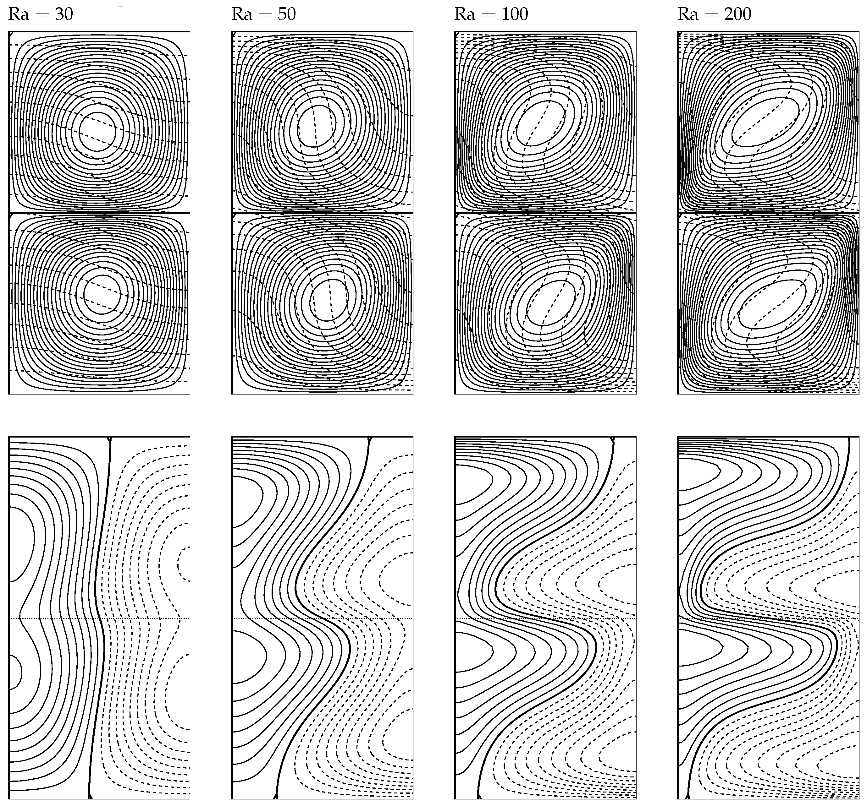
Figure 3 displays a selection of streamlines and isotherms, which were produced using code A in order to show how the flow evolves as the Darcy–Rayleigh number increases. We have chosen to use (i.e., ), so that each of the two sublayers occupy a computational domain with a unit aspect ratio. For this domain, convection begins once Darcy–Rayleigh number is larger than . When , we see that the isotherms deviate by only a small amount from the horizontal, and this indicates that a weak clockwise circulation is induced in each of the two sublayers. As increases, the flow strength also increases, as one would expect for a supercritical bifurcation, and this is shown by the increasing deformation of the isotherms. An apparent up/down symmetry about in the streamlines is lost when is sufficiently large, and we now see the centro-symmetry referred to above in Equation (18).
An alternative way of viewing this flow is shown in the lower row of Figure 3 which displays the perturbation isotherms, i.e.,
When , which is just supercritical, we see that the perturbation isotherms are close to obeying the up/down symmetry, which is satisfied by the linearised disturbance at onset. At onset, these isolines are vertical as they pass through the interface. Thus, it is this symmetry that is referred to above as corresponding to the classical Darcy–Bénard layer with a constant temperature on one surface and a constant heat flux on the other. Now, as increases, we see the hot spots in rising on the left of each sublayer and the cold spots descending. We also see the beginnings of boundary-layer formation on the horizontal surfaces.
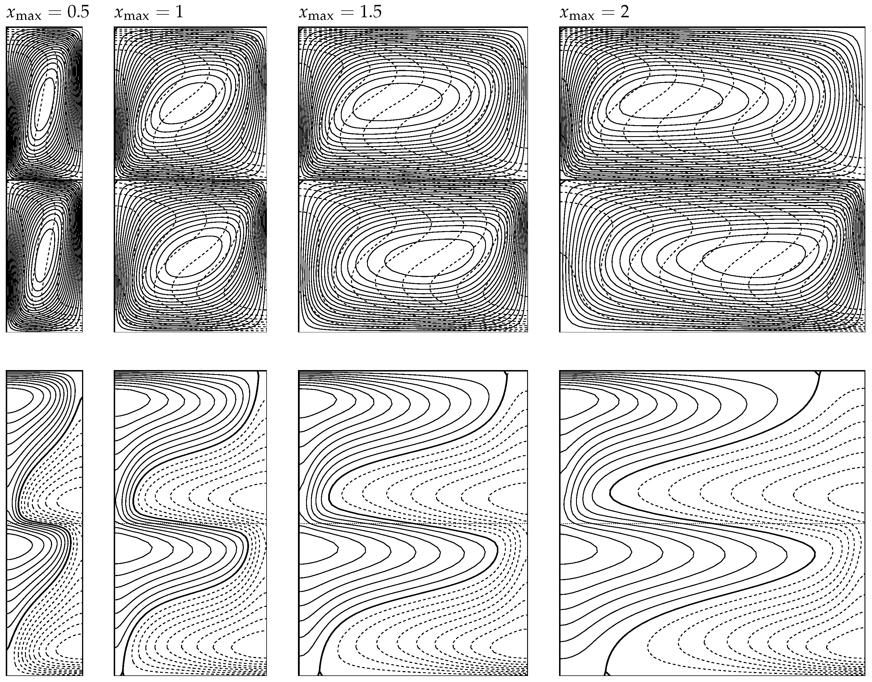
In Figure 4, the Darcy–Rayleigh number has been set at , the largest of which is considered here, and the values of are , 1, and 2, which are equivalent to , π, and . While these streamline and isotherm plots appear superficially to be roughly the same, they hide some unusual behaviour. The largest value of ψ corresponds to out of these four cases, but the largest value of corresponds to . When , the domain is larger and offers less obstruction to the flow, given that most of the time any randomly-chosen fluid particle is moving horizontally. However, this horizontal movement also allows for heat to conduct further into the interior of each sublayer, thereby decreasing the temperature gradient and the Nusselt number. That this is the case is confirmed by the isolines of . Close to the top left-hand side of the upper sublayer, it is clear that the isotherms are almost identical, and that the close spacing of these isotherms indicates that there is high local rate of heat transfer on the upper surface. However, when the two extreme cases are compared, we see that this high rate of heat transfer is maintained over almost all of the upper surface when , but when , the local rate of heat transfer has already changed sign before the top right corner has been reached.
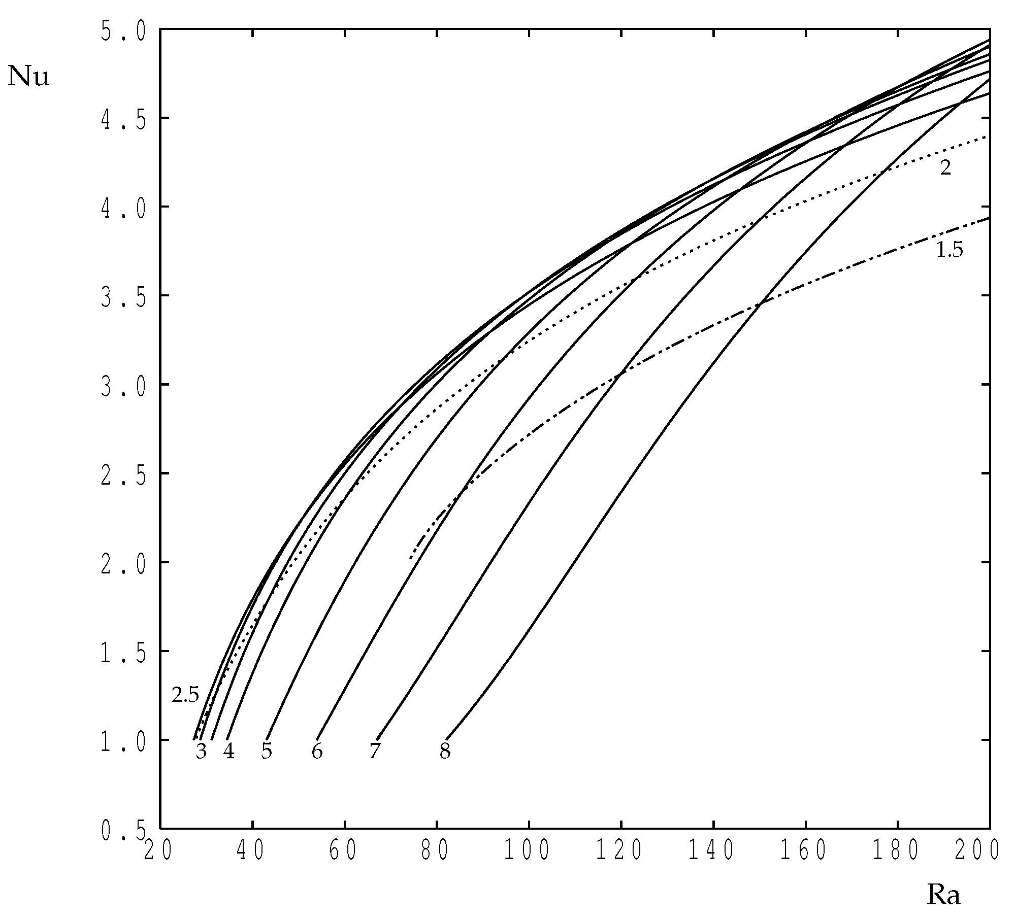
Figure 5 shows how the Nusselt number varies with for a choice of values of the wavenumber. The continuous curves represent values of k which are above the critical value, and all of them show that there is a straightforward supercritical bifurcation to a strongly convecting flow as increases, where represents the conducting state. Confining ourselves to these curves, it is clear that the value of at which the onset of convection occurs decreases as k decreases, precisely in line with the neutral curve shown in Figure 2. Numerically, our extrapolated onset criteria based on extrapolations of the value of back to , which corresponds to conduction, agree with the exact dispersion relation values to within at most. It is of interest to note that these curves cross one another as increases, and it is clear that the wavenumber at which achieves its largest value depends on the Darcy–Rayleigh number; this will be investigated in more detail in Figure 6, below.
The dotted line in Figure 5 corresponds to , which is less than the value of . It has the same behaviour as those drawn with continuous lines, although the value of at which convection starts has begun to increase once more. However, the dotted-dashed line, for which , terminates at approximately ; it is not possible to find steady solutions using our time-dependent code at smaller values of . In our simulations for such cases, we find that, while the one-cell perturbation grows at first, it eventually transforms into a three-cell flow where each of these new cells corresponds to the one cell that is obtained when solving using a wavenumber that is three times larger. For relatively small wavenumbers, the width of the domain, is now quite wide, and, therefore, we obtain a flow where the three new cells each occupy a region of horizontal width . The reason for this will be discussed after Figure 6 is introduced.
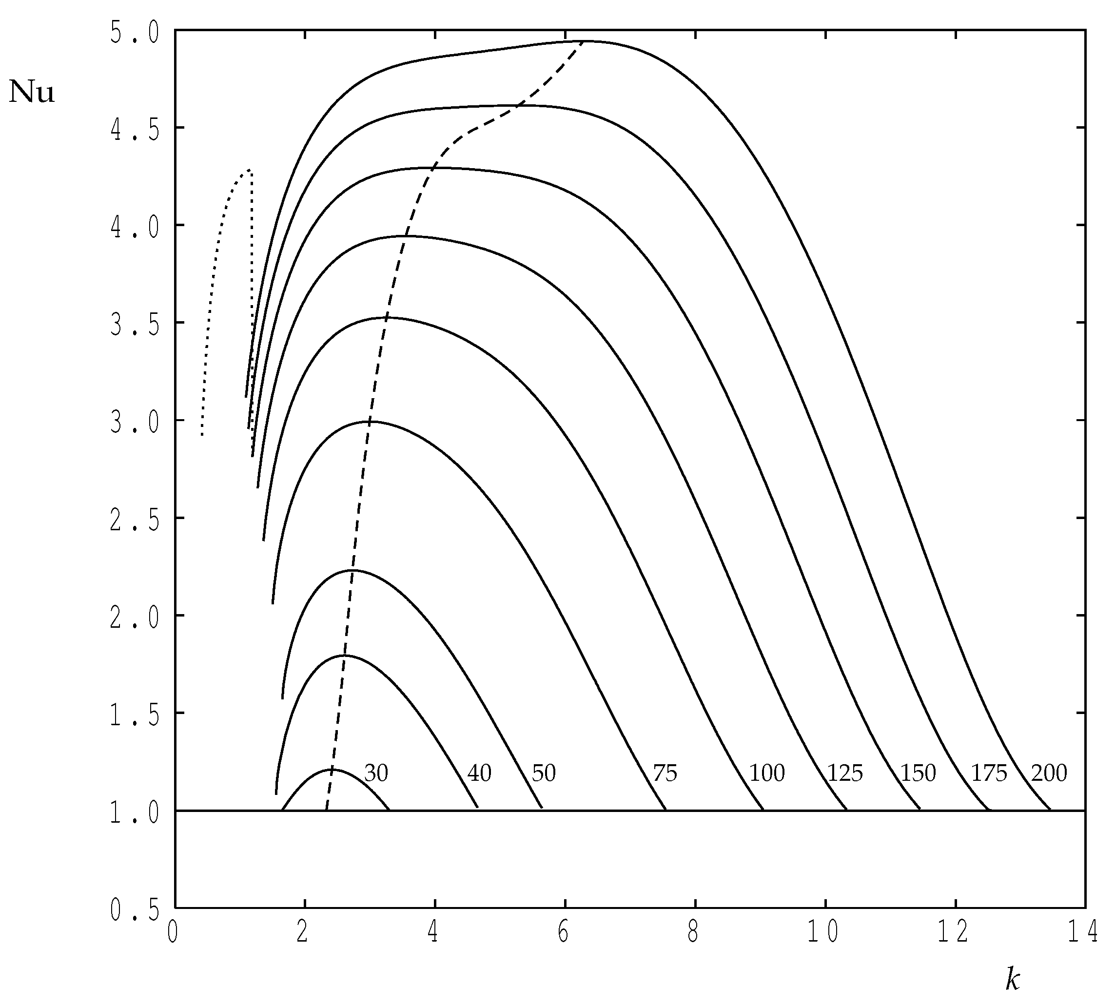
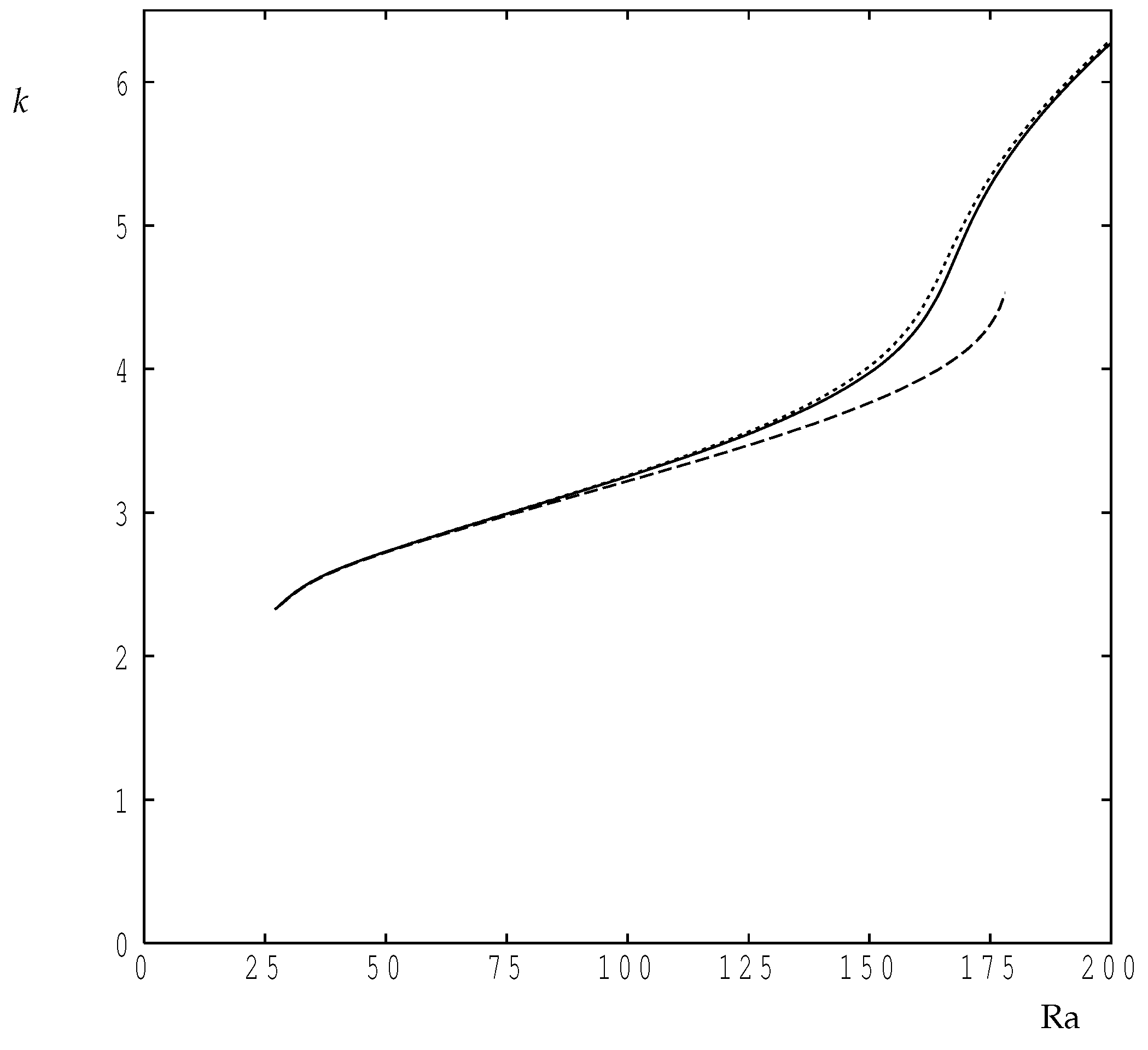
Figure 6 shows how the Nusselt number varies with wavenumber for a choice of values of , and these were obtained using code C. In all cases corresponds to conduction, and departure from this value corresponds to onset. The general behaviour of as a function of k follows that of the classical Darcy–Bénard layer shown in de la Torres and Busse [20], where the maximum rate of heat transfer is obtained at some value of the wavenumber which is intermediate between the two values corresponding to the neutral curve at the chosen value of ; this would not necessarily be the case if parts of the neutral curve correspond to a subcritical bifurcation. The locus of maxima is shown in Figure 6 as a dashed line, and these values were obtained using code D. As increases, the wavenumber at which attains its maximum value increases as increases, which is the same qualitative behaviour as was found in de la Torres and Busse [20]. The detailed variation of the maximising value of k as increases is shown in Figure 7. This variation shows a surprising change in direction once rises above 150, and therefore the accuracy of our computations were re-checked using a coarser grid (—double the step lengths in the cordinate directions), and a finer grid (—approximately times the respective step lengths). The line corresponding to the coarser grid terminates at because of resolution difficulties, but the difference between the coarse values and those of our chosen grid are quite small when . On the other hand, the finer grid is in close agreement with our chosen grid. At , we obtain using our chosen grid and using the finer grid, a relative change of less than .
The second feature found in Figure 6 is that, as the wavenumber increases, our unsteady code is unable to obtain solutions all the way back to the onset criterion. The various curves terminate before reaching the value of k representing the neutral curve, the sole exception being when . This is the same phenomenon as is mentioned above with regard to Figure 5. We attempt to explain this using the case (i.e., ). When , convection begins when , whereas when , it begins when . From the point of view of small-amplitude disturbances, a disturbance at and a disturbance at the same value of will have different exponential growth rates. On applying such a theory, details of which are omitted here, we find that the disturbance grows with an amplitude that proportional to while the disturbance grows as ; these growth rates remain accurate until nonlinear effects become significant and growth is attenuated. Now, if the disturbance is initiated, then the nonlinear terms in the heat transport equation combine to yield terms that include the disturbance as a component, and this grows more quickly than the original disturbance. It appears, therefore, that if k takes a value which is sufficiently close to the left-hand branch of the neutral curve, then the component, which has a substantially greater growth rate, will eventually overwhelm the original disturbance and form the ultimate steady state. At larger values of k, the difference between the two growth rates is much smaller, and the original disturbance continues to develop towards steady state. In general, a nonlinear interaction forming a component has a different symmetry, and this term will generally decay and play only a passive role.
The dotted line in Figure 6 demonstrates the above k to transition as k decreases in the case . The steady-state solution that we obtain when with k decreasing undertakes a sudden transition at to the solution, as described above. This dotted curve is, in effect, a three-times compressed version of the continuous curve. Subject to the fact that this ‘’ solution at has relatively poor spatial resolution, its Nusselt number is essentially the same as was obtained for the ‘k’ solution when .
5. Conclusions
The literature is replete with linear stability analyses for convection in a variety of layered systems involving porous media, but apart from some very early work [1,2,3] on fairly restrictive systems composed of porous sublayers, no nonlinear computations have been reported. The present paper has considered a very simple modification to the classic Darcy–Bénard problem, one where a horizontal, infinitesimally thin but impermeable interface is placed centrally within the porous layer. This has the effect of modifying the linearised stablity problem to one which is exactly equivalent to that variant of the Darcy–Bénard problem where one surface is held at a constant temperature, but the other is subject to a constant heat flux. We have found that this analogy does not extend into the nonlinear regime, where, for Darcy–Rayleigh numbers that are below 200, the flow and temperature fields satisfy appropriated forms of centro-symmetry, rather than the up–down symmetry which applies to the linearised disturbances. We find that the most favoured wavenumber, at least in terms of that which maximises the mean rate of heat transfer, increases as the Darcy–Rayleigh number increases, showing the narrow cells transport more heat than those of roughly aspect ratio.
Conflicts of Interest
The author declares no conflict of interest.
Abbreviations
| C | heat capacity |
| g | gravity |
| k | wavenumber () |
thermal conductivity of the porous medium | |
| K | permeability |
| L | height of one sublayer |
Nusselt number | |
| NX | number of intervals in the x-direction |
| NZ | number of intervals in the z-direction |
| p | pressure |
| Ra | Darcy–Rayleigh number |
| t | time |
| T | dimensional temperature |
upper (cold) boundary temperature | |
lower (hot) boundary temperature | |
| u | horizontal velocity |
| w | vertical velocity |
| x | horizontal coordinate |
width of the computational domain | |
| z | vertical coordinate |
| CGIs | CpG islands |
| β | expansion coefficient |
temperature drop across a sublayer | |
| θ | temperature |
| λ | value defined in Equation (21) |
| μ | dynamic viscosity |
| ρ | density |
| σ | value defined in Equation (21) |
| ψ | streamfunction |
| c | critical value |
| f | fluid |
| pm | porous medium |
| ^ | dimensional quantity |
| + | immediately above the interface |
| − | immediately below the interface |
Appendix A. Accuracy Considerations
The aim of this Appendix is the justification of the choice of numerical grid that has been used for the bulk of the present paper.
The critical Darcy–Rayleigh number for this two-layer configuration is and the critical wavenumber is . The value of this wavenumber is such that one single cell of the corresponding convection pattern has width, . Given that we are using a multigrid methodology to solve the Poisson’s equation for the streamfunction, the number of intervals in each direction must have factors which are powers of two. Therefore, we solved the equations of motion on the three different uniform grids: , and for a single-cell solution at the critical wavenumber, while the Darcy–Rayleigh number was varied within the range, .
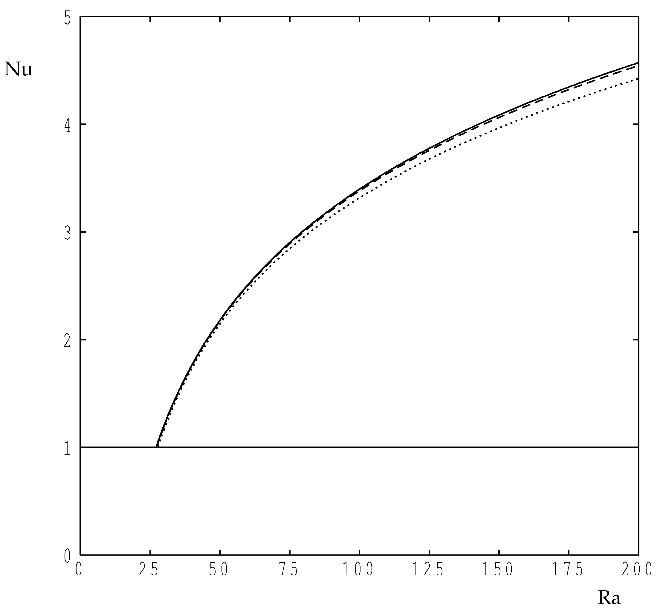
The variation of the computed Nusselt number with is given in Figure A1 for the three grids, and we see that there is very little difference in the value of Nu when when considering the two finest grids. The coarsest grid clearly has a substantial error associated with it. In particular, Table A1 gives that data for , which is the most extreme case considered here, and it is clear that they are commensurate with a second order accurate numerical scheme.
Figure A1.
The value of as a function of for using the three grids: (dotted), (dashed) and (continuous).
Figure A1.
The value of as a function of for using the three grids: (dotted), (dashed) and (continuous).


| NX × NZ | Nu |
|---|---|
| 12 × 16 | 4.4238 |
| 24 × 32 | 4.5451 |
| 48 × 64 | 4.5720 |
A second way of determining the accuracy of our computations (which also provides some validation of the coding) is to use the Nusselt number for values of , which are just above the critical value. The numerical code was run using and convergence was deemed to have taken place when the maximum change in θ between timesteps is less than for 50 successive timesteps. Given that the Nusselt number is a linear function of according to weakly nonlinear theory (which is valid when is sufficiently small), we extrapolated back to from two different postcritical solutions near in order to estimate the value of . The result of this extrapolation process is given in Table A2, and it is clear these data are also commensurate with a numerical method which has second order accuracy in space.
Table A2.
Extrapolated values of the critical Darcy–Rayleigh number and their errors as a function of the numerical grid.
| NX × NZ | Error | |
|---|---|---|
| 12 × 16 | 27.762 | 2.45% |
| 24 × 32 | 27.265 | 0.62% |
| 48 × 64 | 27.129 | 0.15% |
Given that the order of accuracy of the numerical method is reproduced faithfully, not only in its prediction of the value of , but also in the extreme case of , we decided that it was unnecessary to adopt a still finer grid for the present work. Therefore, we have used a grid with 64 intervals in the vertical direction and 48 horizontally. Computations at higher values of the Darcy–Rayleigh number will require more resolution.
References
- Georghitza, St.I. The marginal stability in porous inhomogeneous media. Proc. Camb. Phil. Soc. 1961, 57, 871–877. [Google Scholar] [CrossRef]
- Masuoka, T.; Katsuhara, T.; Nakazono, Y.; Isozaki, S. Onset of convection and flow patterns in a porous layer of two different media. Heat Transf. Jpn. Res. 1979, 7, 39–52. [Google Scholar] [CrossRef]
- Rana, R.; Horne, R.N.; Cheng, P. Natural convection in a multi-layered geothermal reservoir. J. Heat Transf. 1979, 101, 411–416. [Google Scholar] [CrossRef]
- McKibbin, R.; O’Sullivan, M.J. Onset of convection in a layered porous medium heated from below. J. Fluid Mech. 1980, 96, 375–393. [Google Scholar] [CrossRef]
- McKibbin, R.; O’Sullivan, M.J. Heat transfer in a layered porous medium heated from below. J. Fluid Mech. 1981, 111, 141–173. [Google Scholar] [CrossRef]
- Rees, D.A.S.; Riley, D.S. The three-dimensional stability of finite-amplitude convection in a layered porous medium heated from below. J. Fluid Mech. 1990, 211, 437–461. [Google Scholar] [CrossRef]
- Mojtabi, A.; Rees, D.A.S. The onset of the convection in Horton-Rogers-Lapwood experiments: The effect of conducting bounding plates. Int. J. Heat Mass Transf. 2011, 54, 293–301. [Google Scholar] [CrossRef] [Green Version]
- Falsaperla, P.; Mulone, G.; Straughan, B. Rotating porous convection with prescribed heat flux. Int. J. Eng. Sic. 2010, 48, 685–692. [Google Scholar] [CrossRef]
- Riahi, D.N. Nonlinear convection in a porous layer with finite conducting boundaries. J. Fluid Mech. 1983, 129, 153–171. [Google Scholar] [CrossRef]
- Rees, D.A.S.; Mojtabi, A. The effect of conducting boundaries on weakly nonlinear Darcy–Bénard convection. Transp. Porous Media 2011, 88, 45–63. [Google Scholar] [CrossRef]
- Rees, D.A.S.; Mojtabi, A. The effect of conducting boundaries on Lapwood-Prats convection. Int. J. Heat Mass Transf. 2013, 65, 765–778. [Google Scholar] [CrossRef] [Green Version]
- Saleh, H.; Saeid, N.H.; Hashim, I.; Mustafa, Z. Effect of conduction in bottom wall on Darcy–Bénard convection in a porous enclosure. Transp. Porous Media 2011, 88, 357–368. [Google Scholar] [CrossRef]
- Jang, J.Y.; Tsai, W.L. Thermal instability of two horizontal porous layers with a conductive partition. Int. J. Heat Mass Transf. 1988, 31, 993–1003. [Google Scholar]
- Postelnicu, A. Thermal stability of two fluid porous layers separated by a thermal barrier. In Proceedings of the 3rd Baltic Heat Transfer Conference, Gdansk, Poland, 22–24 September 1999; pp. 443–450.
- Patil, P.M.; Rees, D.A.S. The onset of convection in a porous layer with multiple horizontal solid partitions. Int. J. Heat Mass Transf. 2014, 68, 234–246. [Google Scholar] [CrossRef] [Green Version]
- Straughan, B. Nonlinear stability of convection in a porous layer with solid partitions. J. Math. Fluid Mech. 2014, 16, 727–736. [Google Scholar] [CrossRef]
- Genç, G.; Rees, D.A.S. The onset of convection in horizontally partitioned porous layers. Phys. Fluids 2011, 23, 064107. [Google Scholar] [CrossRef] [Green Version]
- Rees, D.A.S.; Genç, G. Onset of convection in porous layers with multiple horizontal partitions. Int. J. Heat Mass Transf. 2011, 54, 3081–3089. [Google Scholar] [CrossRef]
- Rees, D.A.S.; Bassom, A.P.; Genç, G. Weakly nonlinear convection in a porous layer with multiple horizontal partitions. Transp. Porous Media 2014, 103, 437–448. [Google Scholar] [CrossRef] [Green Version]
- De la Torres Juarez, M.; Busse, F.H. Stability of two-dimensional convection in a fluid-saturated porous medium. J. Fluid Mech. 1995, 292, 305–323. [Google Scholar] [CrossRef]
Figure 1.
Depicting a porous layer split into two identical sublayers by an infinitesimally thin and impermeable interface.
Figure 1.
Depicting a porous layer split into two identical sublayers by an infinitesimally thin and impermeable interface.
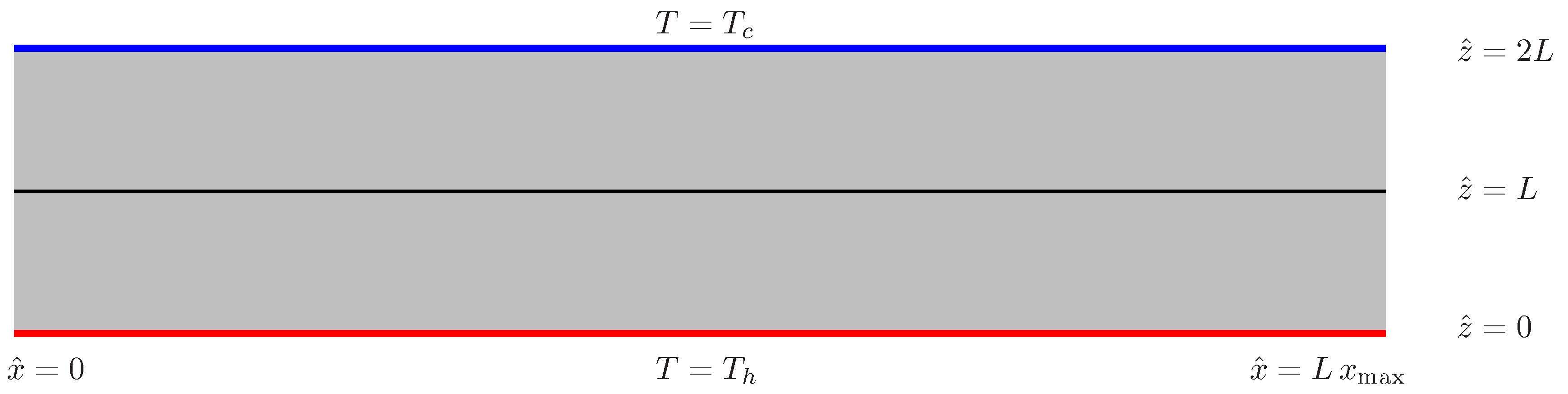
Figure 2.
The first four neutral curves showing the variation of with the wavenumber.
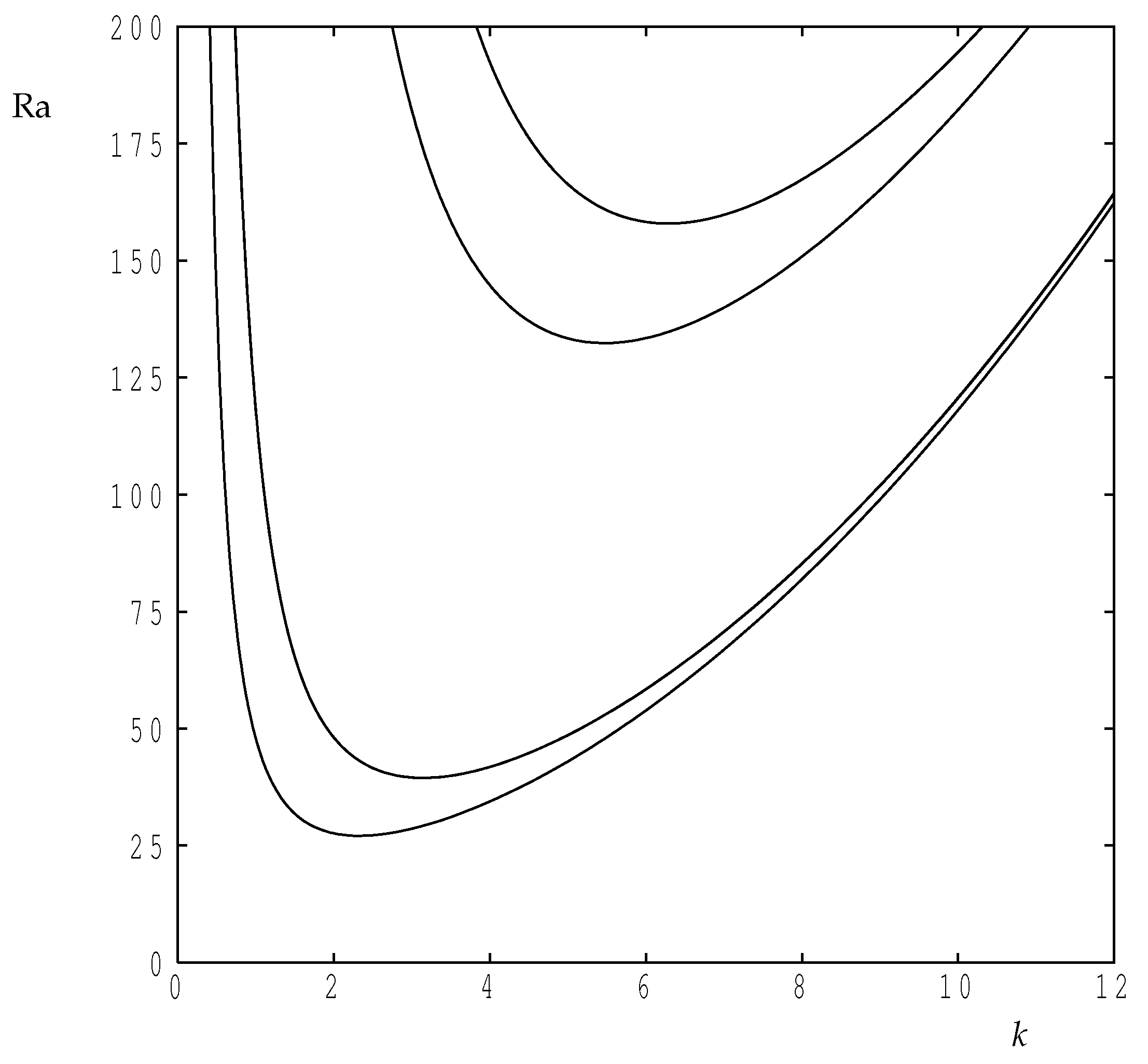
Figure 3.
Upper row: streamlines (continuous) and isotherms (dashed) for the case for the given values of . Lower row: the corresponding isotherms for where continuous lines correspond to where , dashed lines to where it is negative, the thick line to where it is zero, and the dotted line depicts the interface. In all cases, 20 equal intervals were taken for the isolines.

Figure 4.
Streamlines, isotherms and perturbation isotherms for and for the given values of . Isolines follow the same conventions as in Figure 3.
Figure 4.
Streamlines, isotherms and perturbation isotherms for and for the given values of . Isolines follow the same conventions as in Figure 3.

Figure 5.
The variation of the Nusselt number with the Darcy–Rayleigh number for selected wavenumbers. The continuous lines correspond to (extreme left at ), 3, , 4, 5, 6, 7 and 8 (extreme right). The dotted line corresponds to and the dotted-dashed line to .
Figure 5.
The variation of the Nusselt number with the Darcy–Rayleigh number for selected wavenumbers. The continuous lines correspond to (extreme left at ), 3, , 4, 5, 6, 7 and 8 (extreme right). The dotted line corresponds to and the dotted-dashed line to .

Figure 6.
The variation of the Nusselt number with the wavenumber for selected values of . The dashed line is the locus of points which correspond to taking its maximum value. The dotted line illustrates how changes when a disturbance with wavenumber k yields a flow with wavenumber when ; these curves have been suppressed for other values of for clarity of presentation.

Figure 7.
The value of k at which is maximised as a function of . The continuous line corresponds to the standard grid, while the dashed line corresponds to a grid. More accurate computations using a grid are shown using the dotted line.
Figure 7.
The value of k at which is maximised as a function of . The continuous line corresponds to the standard grid, while the dashed line corresponds to a grid. More accurate computations using a grid are shown using the dotted line.
© 2016 by the author; licensee MDPI, Basel, Switzerland. This article is an open access article distributed under the terms and conditions of the Creative Commons Attribution license ( http://creativecommons.org/licenses/by/4.0/).
Share and Cite
MDPI and ACS Style
Rees, D.A.S. Nonlinear Convection in a Partitioned Porous Layer. Fluids 2016, 1, 24. https://doi.org/10.3390/fluids1030024
AMA Style
Rees DAS. Nonlinear Convection in a Partitioned Porous Layer. Fluids. 2016; 1(3):24. https://doi.org/10.3390/fluids1030024
Chicago/Turabian StyleRees, D. Andrew S. 2016. "Nonlinear Convection in a Partitioned Porous Layer" Fluids 1, no. 3: 24. https://doi.org/10.3390/fluids1030024