1. Introduction
The simulation of polymer dynamics represents a long-standing problem in computational rheology. The main challenges are related to the choice of an appropriate fluid-polymer interaction model as well as of the simulation method itself. An important fact which is generally known [
1] is that, for a diluted solution, the hydrodynamic interaction (HI) has strong effects on the dynamics of the polymer. Experiments have confirmed that, under diluted conditions, polymer dynamics is best described by the Zimm model [
2], where the effects of HI are taken into account by using the Oseen tensor formulation, and the solvent is assumed to behave as an incompressible Stokes flow.
A straightforward approach to take HI into account is to simulate solvents and polymers using molecular dynamics (MD). Such studies were done and provided valuable information for the theory of polymer dynamics [
3]. An obvious disadvantage of this approach is the computational cost; in fact, due to limited numerical resources, it is not possible to achieve the relevant length and time scales of experiments. Some modifications, such as coarse-grained molecular dynamics (CMD) [
4], have been proposed in the past to reduce the required computational time, but the problem still remains.
More effective schemes include a stochastic thermal force explicitly applied on the suspended bead while the effect of HI among them is implicitly taken into account via Oseen tensor-based models or higher-order expansions of the incompressible Stokes equations. Afterwards, a resulting set of algebraical equations needs to be inverted. These approaches include, for example, Brownian dynamics (BD) [
5,
6,
7,
8,
9] and Stokesian dynamics (SD) [
10,
11]. Their main advantage is related to the good scalability of the number of equations with the number of suspended particles, allowing for the simulation of large systems [
12]. On the other hand, modelling complex external geometries is not an easy task in implicit-solvent methods and requires essential modification of the standard framework [
13,
14,
15].
To remedy these problems, various researchers have focused in the past on mesoscopic methods which employ numerically effective coarse-grained models retaining the relevant hydrodynamics modes. Examples are multiparticle collision dynamics [
16] and lattice Boltzmann methods (LBM) [
17,
18]. Due to the presence of an underlying grid for the computation of the hydrodynamic interactions, LBM is computationally very effective; however, it generally requires hybrid schemes to describe the dynamics of immersed structures. Using different numerical approaches for solvent and suspended particles in fact requires special care in fluid-structure interaction models in order to ensure exact transfer of momentum and more generally formal thermodynamic consistency of the coupled-scheme.
A mesoscopic particle method called dissipative particle dynamics (DPD) which uses pairwise soft conservative, dissipative and random forces, has gained increasing popularity for its ability of simulating much larger physical length and time scales [
19]. The DPD model shows good performance on investigating the dynamic properties of polymers and conformation of DNA in a microchannel [
20,
21]. A remarkable phenomenon called cross-stream migration of polymers was found recently in a non-uniform shear flow using the DPD model, and the effects of Reynolds number, Schmidt number, polymer chain length and polymer concentration were investigated [
22,
23,
24,
25]. In addition, the so-called “reverse Poiseuille flow” with a DPD polymer model is a convenient virtual rheometer for the acquisition of steady state rheological data [
26].
In this paper, a new type of DPD method, called smoothed dissipative particles dynamics (SDPD) [
27,
28,
29], is used to investigate the static and dynamic behavior of polymers. This model is a mesoscopic extension of a popular particle-based method applied to continuum flow,
i.e., smoothed particle hydrodynamics (SPH) [
30]. Due to its connection to SPH, SDPD allows using an arbitrary equation of state for the pressure and to specify transport coefficients directly without the need to perform kinetic analysis or preliminary runs. Thermal fluctuations can be included in a physically consistent way, that is, in agreement with a fluctuation-dissipation theorem (FDT) and with basic properties of statistical mechanics where fluctuations of hydrodynamic variables increase naturally by reducing the size of the problem down to the mesoscopic scale [
29]. These properties of SDPD make it a suitable tool to simulate physically relevant length and time scales as seen in experiments. If thermal fluctuations are not considered, SDPD reduces to a version of SPH where pressure/velocity profiles for incompressible flows are correctly reproduced [
31,
32].
In this paper, the thermodynamically-consistent SDPD model proposed in Reference [
33] for a polymer molecule in solution is extended to three-dimensional situations allowing for effective simulations of polymer solutions under dilute and concentrated conditions. The paper is organized as follows: In
Section 2, the SDPD model for the solvent and flexible polymer chain is outlined. In
Section 3, the results for the static and dynamic properties of the simulated single polymer are presented. Steady shear-rate rheological properties of concentrated polymer solutions and polymer melts are provided and discussed in
Section 4. Finally, in
Section 5, the results are summarized and conclusions are drawn.
3. Simulation of a Single Polymer
In this section, the static and dynamic properties of a single polymer suspended in the Newtonian medium are investigated. A cubic periodic domain with total number of fluid particles is used for all the simulations in this section. The simulated single polymers have variable lengths with number of beads and 100. The shortest polymer was not considered for some analysis since most of the theoretical models for the polymer are only valid in the asymptotic limit of a long chain.
The polymer and solvent particles are placed initially on a regular grid and a preliminary simulation is run until the system is fully thermalized. Afterward, the resulting configurations of the system are chosen as initial conditions for the subsequent simulations each running with a typical number of time steps equal to . In order to obtain accurate statistics, the final results are averaged from 10 parallel runs.
3.1. Static Properties
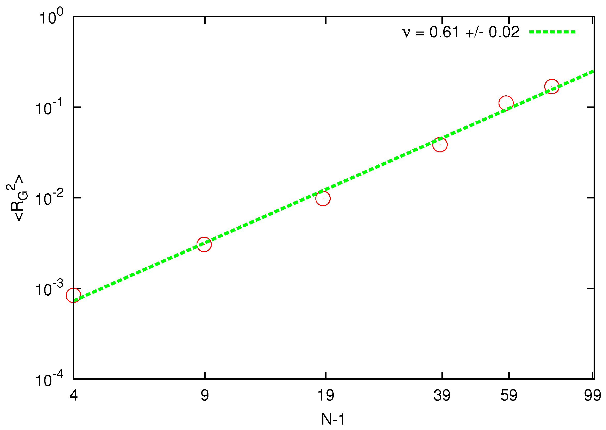
The equilibrium static properties of the polymer are characterized by the mean square radius of gyration of the polymer chain. The radius of gyration is defined as
where
is the distance between beads. The end-to-end distance is defined as
where
N denotes the number of beads of the polymer chain. The static exponent
ν relates the characteristics size of polymer and the number of the beads by
The calculated mean square radius of gyration is shown in
Figure 1.
Figure 1.
Scaling of the radius of gyration for chain lengths corresponding to beads. The solid line represents the best fit of the static exponent.
Figure 1.
Scaling of the radius of gyration for chain lengths corresponding to beads. The solid line represents the best fit of the static exponent.
The estimated static exponent is around above the asymptotic value for a self-avoiding walk .
Another way to obtain the static exponent is to use the static structure factor
This method has certain advantages since, even for a single polymer, it probes different length scales. In the scaling regime
, where
is the characteristic length of the neighboring beads distance, the relationship
holds.
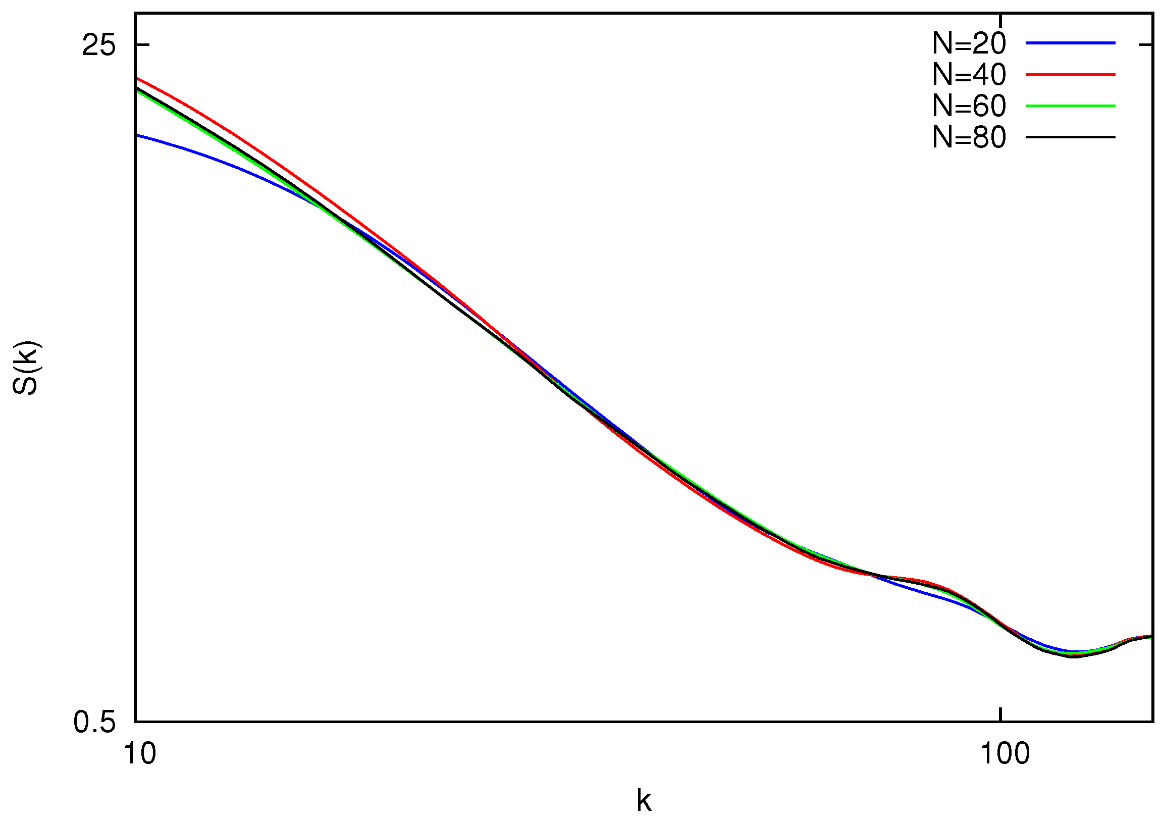
Figure 2 shows static structure factors for polymers with the number of beads
. The results for the polymers with a small number of beads
show deviations from the overall trend and are not presented. This can be explained by the fact that for short chains the effect of the polymer ends is non negligible. By fitting the power-law in logarithmic scale, one can obtain the values of
ν listed in
Table 1.
Figure 2.
Equilibrium static structure factor vs. wave vector magnitude k for polymers with length . All the curves collapse on a master line within the region of .
Figure 2.
Equilibrium static structure factor vs. wave vector magnitude k for polymers with length . All the curves collapse on a master line within the region of .
Table 1.
Estimated static exponent from the fit of the linear part of within the region of .
Table 1.
Estimated static exponent from the fit of the linear part of within the region of .
| N | 20 | 40 | 60 | 80 |
|---|
| ν | 0.59 | 0.57 | 0.62 | 0.61 |
As a comparison, with the renormalization group theory and Monte Carlo simulation, an accurate value of
has been obtained [
41,
42]. Our results are in good agreement with this prediction as well as with previous CMD, BD and DPD simulations [
17,
20,
43,
44]. Since the obtained static exponent is typical for a self-avoiding chain, one may conclude that the excluded volume effects between SDPD particles are taken into account correctly.
3.2. Diffusion Coefficient
One of the most important dynamic properties of a polymer chain is the diffusion coefficient (
D). This can be estimated from the mean-square displacement of the polymer center of mass:
The relation between
and
was plotted and extrapolated to
where
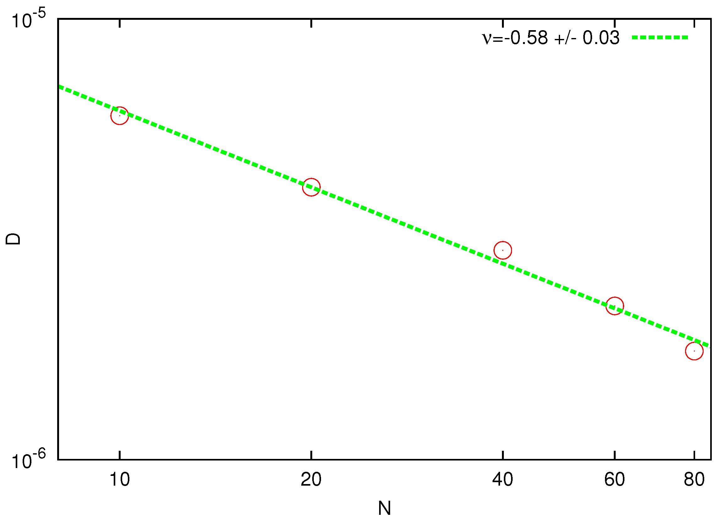
. The resulting power-law dependence of
D versus number of beads is shown in
Figure 3. The fitted slope
is in good agreement with the prediction of the Zimm theory. Note that the same value of the exponent was obtained in the DPD simulations [
44] by extrapolating the data from a much smaller size domain to the thermodynamic limit.
Figure 3.
Log-log plot of the diffusion coefficient D as a function of the chain length N. The solid line represents the best fit with the theoretical power law.
Figure 3.
Log-log plot of the diffusion coefficient D as a function of the chain length N. The solid line represents the best fit with the theoretical power law.
3.3. Longest Polymer Relaxation Time
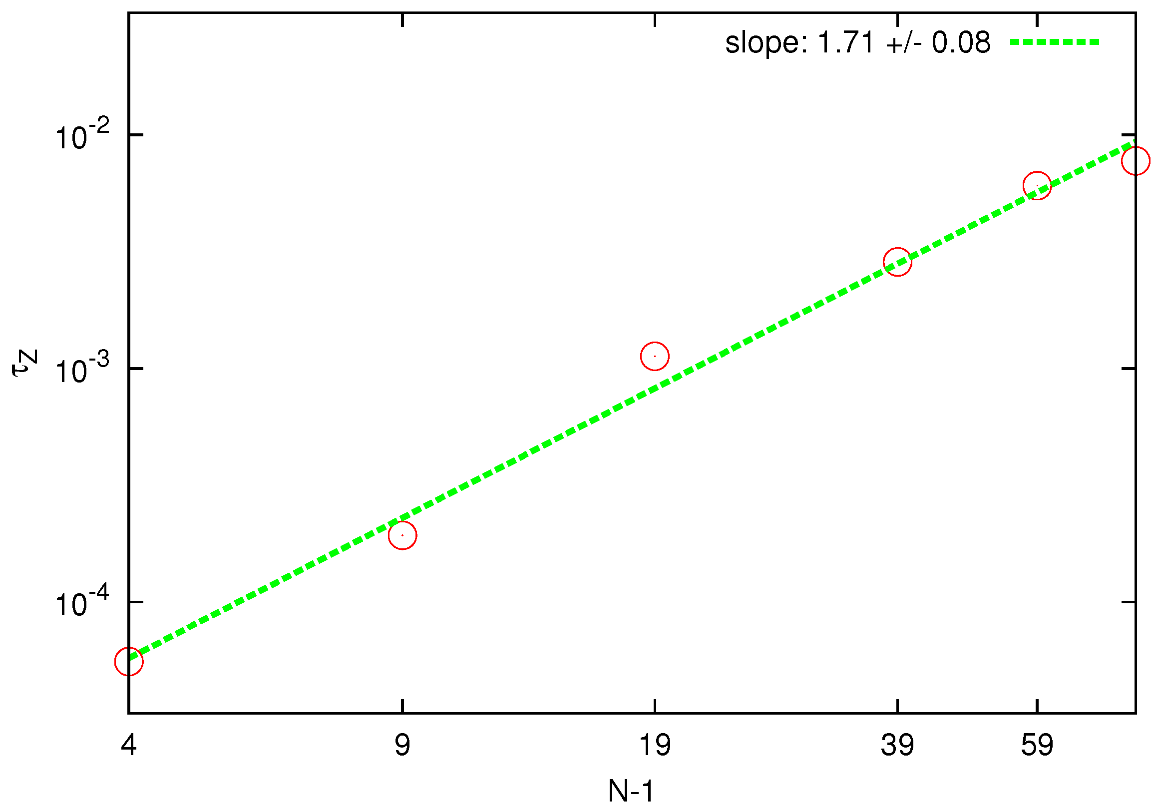
The longest relaxation time of the polymer represents another important dynamical feature and is obtained by fitting the auto-correlation function of the radius of gyration
where the brackets indicate averages over all parallel simulations at various time origins
. For
within the range
the curves were approximated by the expression
and the fitted values of
are shown in the
Figure 4.
Figure 4.
Log-log plot of the longest relaxation time, computed from the autocorrelation of the radius of gyration, as a function of the chain length . The solid line is the best fit to determine the static exponent according to the Zimm model.
Figure 4.
Log-log plot of the longest relaxation time, computed from the autocorrelation of the radius of gyration, as a function of the chain length . The solid line is the best fit to determine the static exponent according to the Zimm model.
One can verify whether the HI effects have been introduced in the current simulations by fitting the scaling of
on polymer length with the static exponent. For the Zimm model, one expects
, while for the Rouse model
should hold. In
Figure 4, the predicted static exponent resulting from the Zimm scaling is
which is in good agreement with the independent value obtained above by the static analysis. On the contrary, application of the Rouse model delivers a much smaller value. Agreement with the Zimm model is consistent with the full description of hydrodynamic interactions between beads within the chain which is not taken into account in the Rouse model.
3.4. Rouse Modes
The Rouse coordinates for a discrete polymer are defined as
where
are the number of Rouse modes and
is the position of bead
n.
are the eigenfunctions of the Gaussian model which provide important information on the static and dynamic behavior. Note that
is simply the polymer center of mass whereas for
,
, and
characterize the internal motion of the polymer on various characteristic lengths.
To test whether the HI is correctly reproduced by the SDPD model, we have analyzed relaxation times
of the Rouse modes.
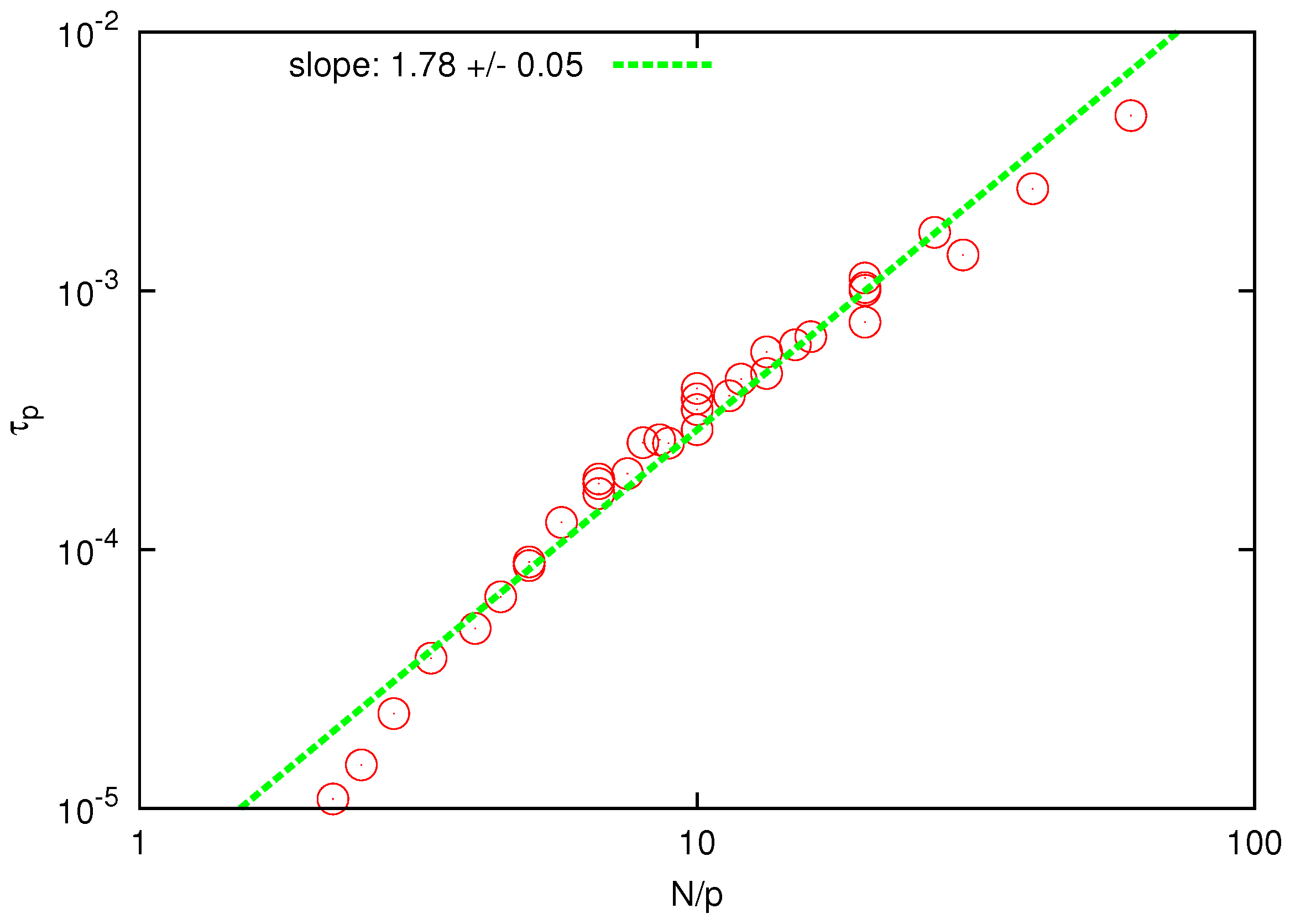
Figure 5 shows the scaling plot of
with
.
Figure 5.
Log-log plot of the relaxation time of Rouse modes vs for . The solid line is the best fit to determine the scaling exponent.
Figure 5.
Log-log plot of the relaxation time of Rouse modes vs for . The solid line is the best fit to determine the scaling exponent.
The collapse of the curves for different polymers and Rouse modes is clear and the scaling exponent is found to be
, in good agreement with the prediction of the Zimm model (
) and substantially below the prediction of the Rouse model (
). When
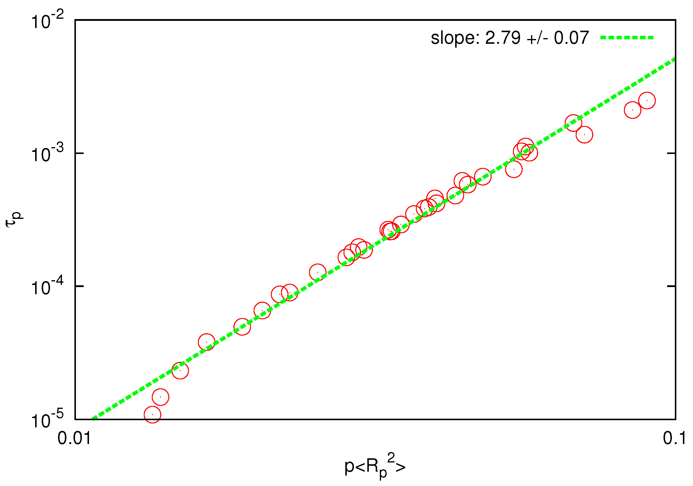
is plotted against
, as shown in
Figure 6, the fitted scaling exponent is in the range
, which is only slightly below the prediction of the Zimm model (
), whereas the Rouse model predicts a much larger value
. The last observation can be considered as an independent test for the presence and accurate description of HI since the prediction of the Zimm scaling (
) is not a consequence of the correct prediction of the static exponent [
44].
Figure 6.
Log-log plot of the relaxation time of Rouse modes vs for . The solid line is the best fit to determine the scaling exponent.
Figure 6.
Log-log plot of the relaxation time of Rouse modes vs for . The solid line is the best fit to determine the scaling exponent.
4. Polymer Melt and Solution
The polymer melt is modelled as an ensemble of flexible polymer chains without solvent particles. The corresponding rheological properties are investigated by using the so-called “reverse Poiseuille flow” (RPF) which consists of two parallel Poiseuille flows driven by uniform body forces of equal magnitude but acting in opposite directions [
26]. DPD simulations using RPF have been successfully used in diluted polymer solutions [
23], colloidal suspensions [
45] and polymer fluids [
26].
In the current simulation, the RPF is driven by a constant force
acting on every SDPD particle in the
x-direction defined as
where
is the size of the domain in the
direction. A cubic periodic domain is used with a total number of fluid particles
. The domain size is
,
and
. The timestep is set to
and all simulations are run at least for
timesteps. For sake of completeness, the full set of parameters used in the simulations are listed in
Table 2 based on SI units.
For a pure solvent simulation under the considered driven force, the estimated Reynolds number based on maximal fluid velocity is
and the Schmidt number is
which is in the same order as Schmidt numbers for real fluids [
46].
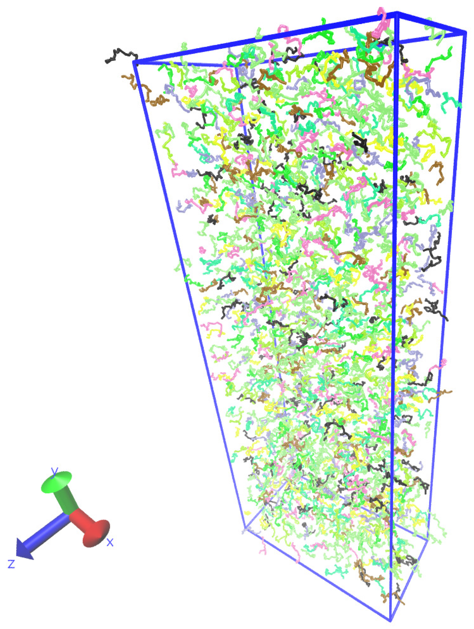
Figure 7 shows a typical snapshot of the polymer system.
For power-law models of non-Newtonian fluids, the RPF velocity profile reads [
26]
where
is the length of the simulation domain in the
direction,
p is the power-law index (e.g.,
corresponds to a constant-viscosity Newtonian model),
κ is the power-law shear stress coefficient and
n is the number density.
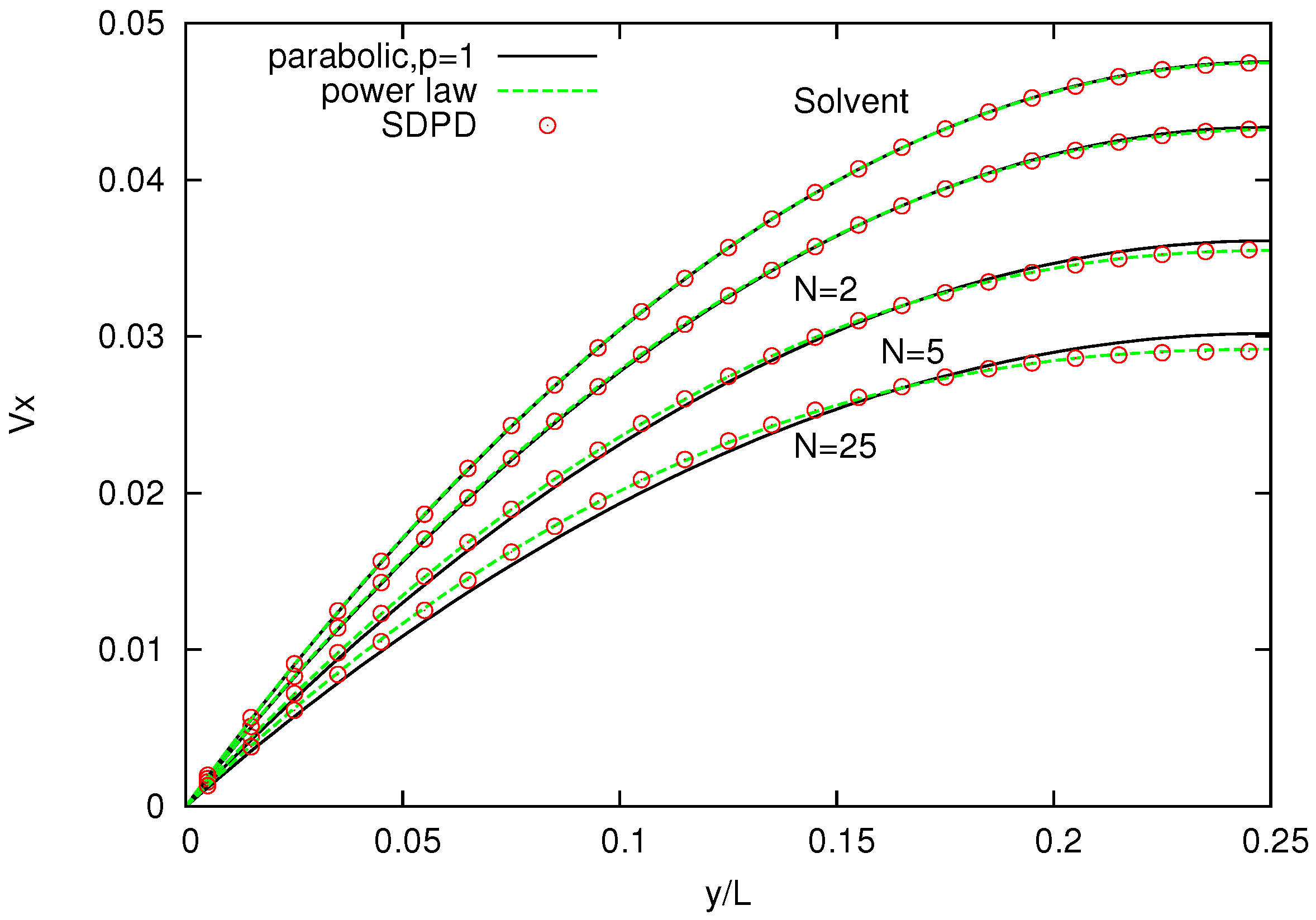
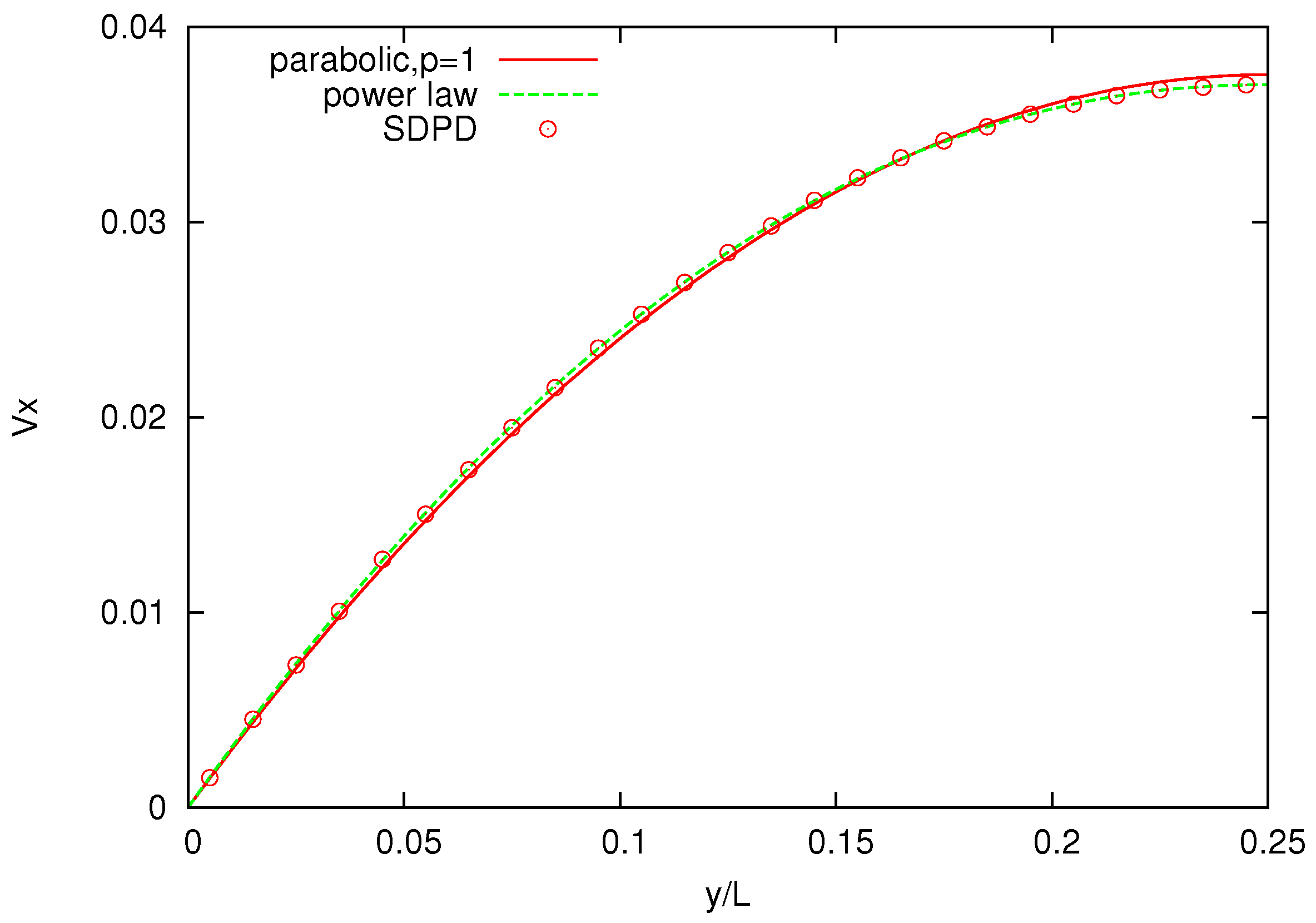
Figure 8 shows the velocity profile across the channel for polymer melts of
-bead chains and, as a comparison, for a pure solvent. The solvent velocity profile is parabolic (
), whereas the melt velocity profiles are increasingly non-Newtonian (for increasing number of bead chains) and are in good agreement with those reported for DPD simulations, with
p being slightly higher for SDPD [
26].
Table 2.
Parameters used for the simulation of polymer melts. Here is the initial smoothed dissipative particle dynamics method (SDPD) particle spacing and is sound speed.
Table 2.
Parameters used for the simulation of polymer melts. Here is the initial smoothed dissipative particle dynamics method (SDPD) particle spacing and is sound speed.
| | ρ | | η | k | | f |
|---|
| | 1000 | 0.3 | 0.015 | | | 6.12 |
Figure 7.
Snapshot of the polymer melt simulation:
x is a direction of the body force and
y is the direction of the velocity gradient. The visualization was done with the Visual Molecular Dynamics (VMD) program [
47].
Figure 7.
Snapshot of the polymer melt simulation:
x is a direction of the body force and
y is the direction of the velocity gradient. The visualization was done with the Visual Molecular Dynamics (VMD) program [
47].
Figure 8.
Velocity profiles for solvents and three melts with chains characterized by . Power-law indices p are , respectively.
Figure 8.
Velocity profiles for solvents and three melts with chains characterized by . Power-law indices p are , respectively.
Higher power indices indicate that the simulated melts are less viscous and exhibit a slightly weaker shear-thinning behavior compared to those reported in the DPD simulations. One possible reason for this discrepancy is that the value of parameters, spring constant k and maximum allowed spring length , employed in the FENE bond differs from those used in DPD.
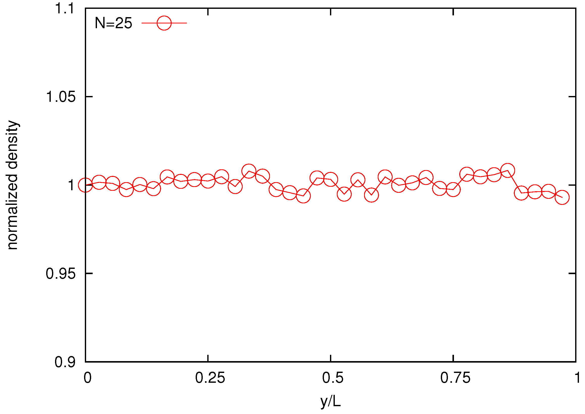
Distribution of polymer beads across the domain is investigated in
Figure 9 where a uniform bead density field is observed for the 25-bead melt. This is an essential phenomenon for the pure-chain melt as a result of incompressibility.
Figure 9.
Normalized bead density profile for the melt composed by 25-bead chains.
Figure 9.
Normalized bead density profile for the melt composed by 25-bead chains.
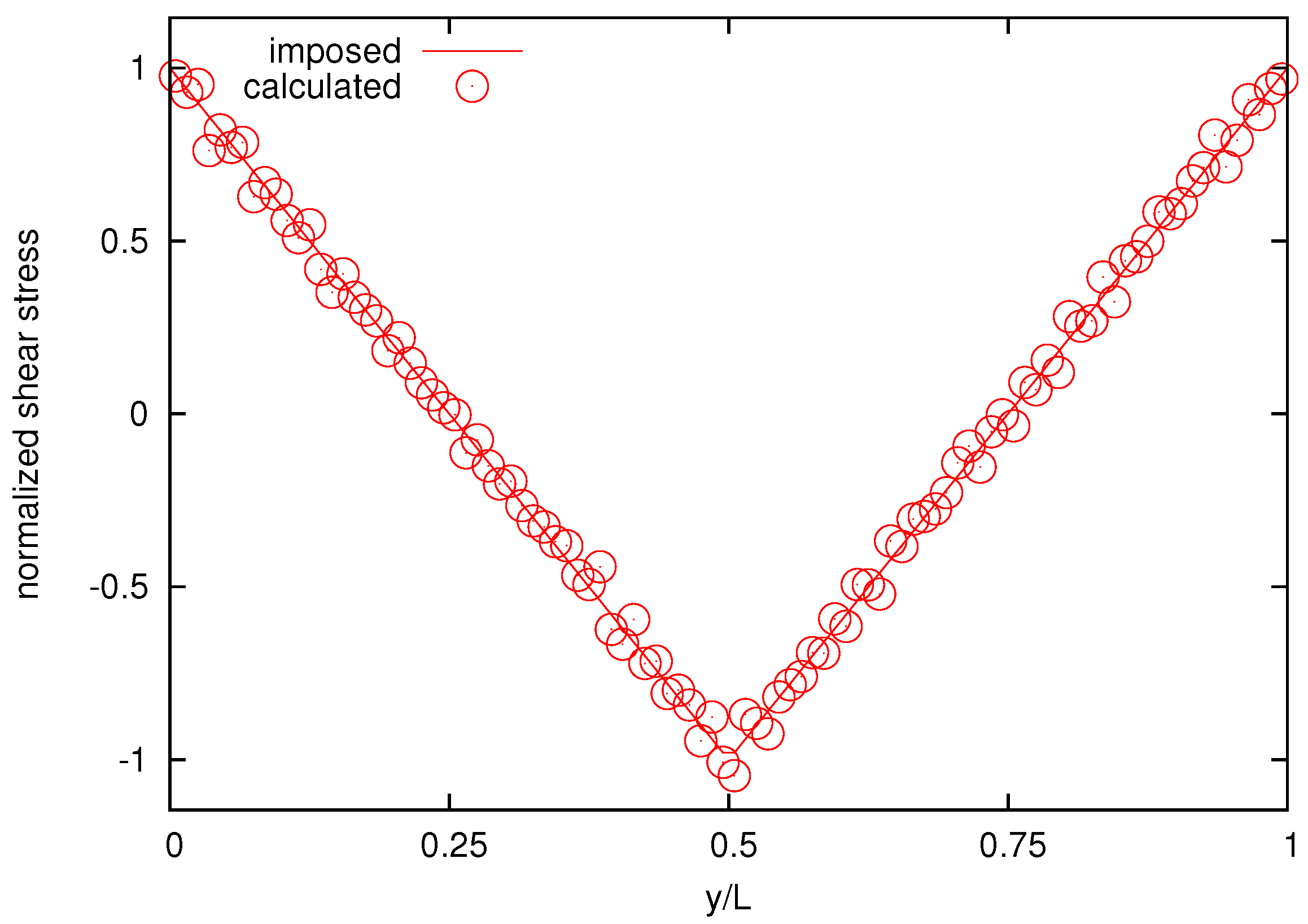
As a further test, next we measure stress field present in the system [
48]. In the RPF, an off-diagonal component of the shear stress
for
and
for
should be recovered.
Figure 10 reports the imposed and the calculated normalized shear-stress distribution for the melt with
bead chains for comparison, showing good agreement.
Figure 10.
The calculated and imposed normalized shear-stress distribution for the melt composed by 25-bead chains.
Figure 10.
The calculated and imposed normalized shear-stress distribution for the melt composed by 25-bead chains.
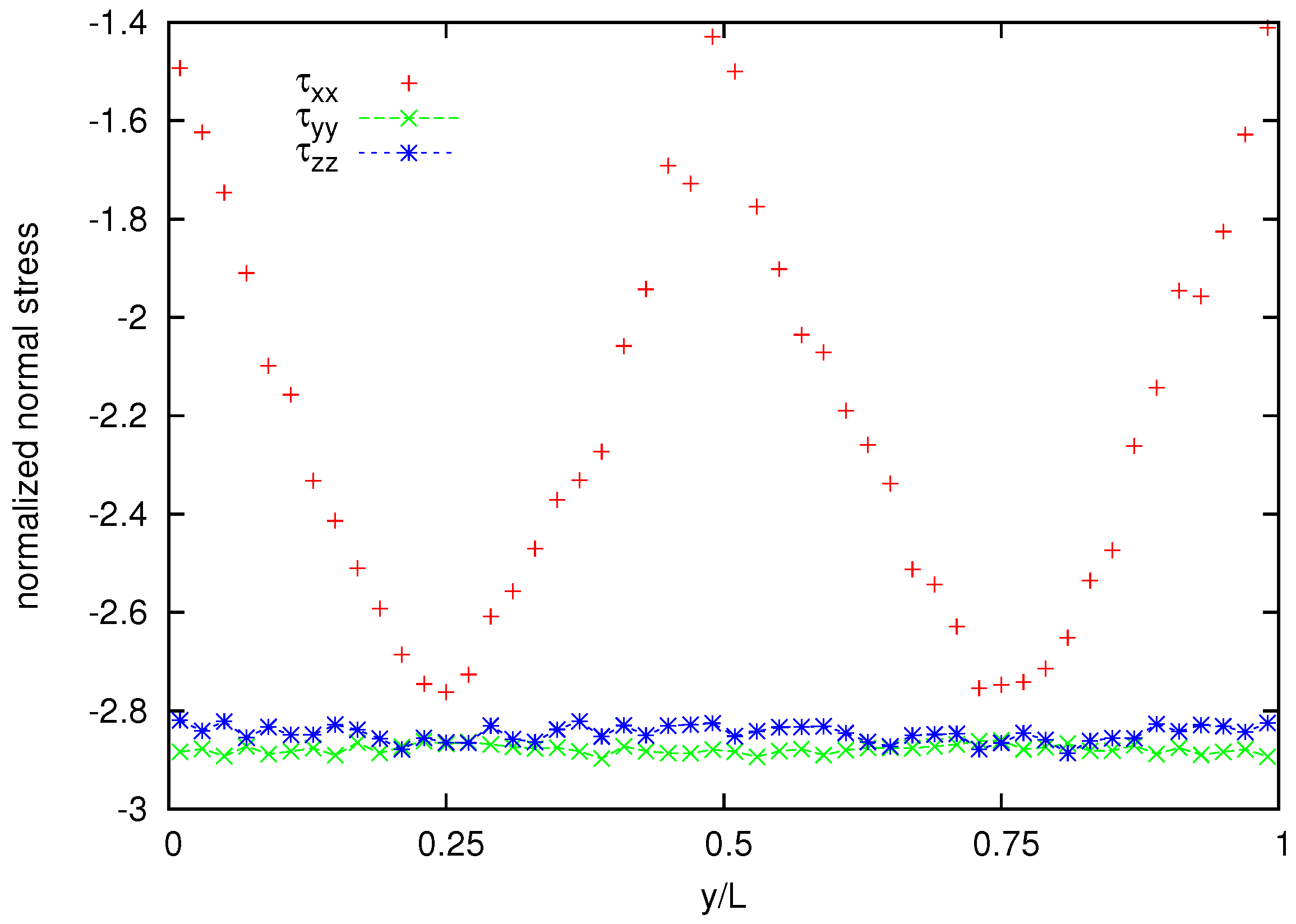
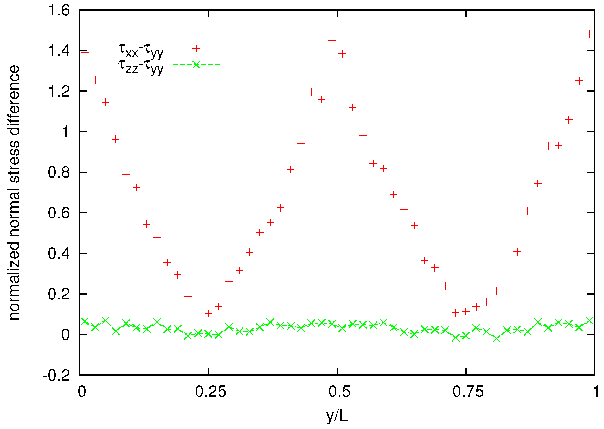
Figure 11 shows also the cross channel distribution of normalized normal-stress components whereas the normalized normal stress difference is shown in
Figure 12. A coarser representation is used for normal stress and normal stress difference, because their averages appear to be more noisy than that for the velocity and the shear stress.
Figure 11.
Normalized stress distribution for the melt of N = 25 bead chain.
Figure 11.
Normalized stress distribution for the melt of N = 25 bead chain.
Figure 12.
Normalized normal stress difference distribution for the melt of N = 25 bead chain.
Figure 12.
Normalized normal stress difference distribution for the melt of N = 25 bead chain.
The ability of the SDPD model for simulating a concentrated polymer solution is investigated by using a 50% concentration of 25-bead chains suspended in a solvent of SDPD fluid particles. The driving constant force is the same as in the case of a melt. The viscosity of the solution is smaller as suggested by the higher maximal velocity value
compared to the value
obtained for a melt composed by the same 25-bead chains, as shown in
Figure 13. Moreover, the larger value of power index of the velocity profile (
with respect to
corresponding to the melt) suggests that the solution has an increasingly Newtonian-like behavior, with viscosity being only slightly shear-rate dependent.
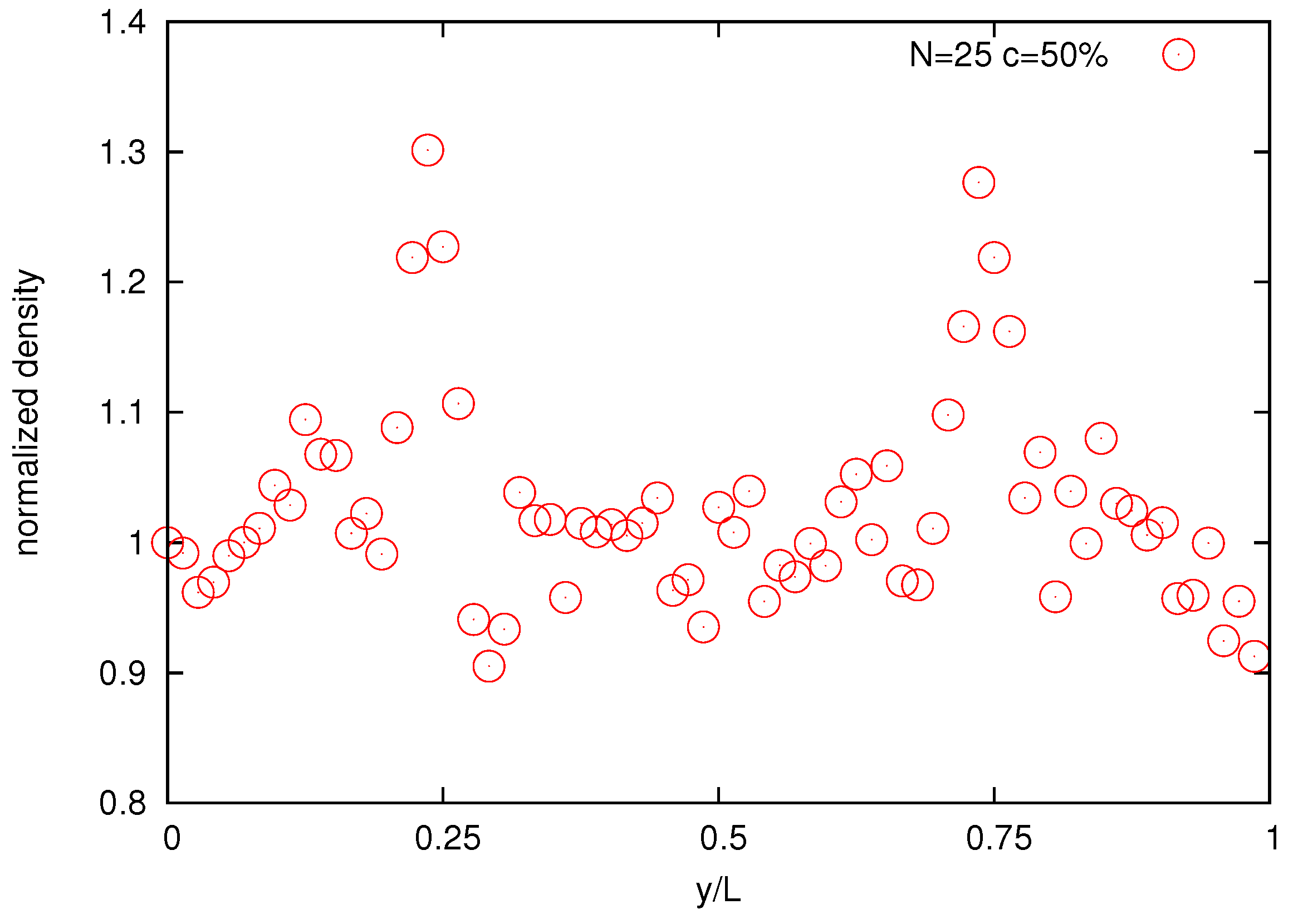
Finally,
Figure 14 shows the normalized bead density of the solution. The two large density peaks occur around at
and
positions where the velocity gradients are zero with maximal density around
. This is a manifestation of the polymer cross-stream migration phenomenon observed in experiments [
49] and simulations [
24,
26,
50].
Figure 13.
Velocity profile for the melt of N = 25 bead chain for bulk concentration 50%. Power-law index p is .
Figure 13.
Velocity profile for the melt of N = 25 bead chain for bulk concentration 50%. Power-law index p is .
Figure 14.
Normalized bead density profile for the melt of N = 25 bead chain for bulk concentration 50%.
Figure 14.
Normalized bead density profile for the melt of N = 25 bead chain for bulk concentration 50%.


