Synthesizing High-Utility Patterns from Different Data Sources


Department of Computer Engineering, St. Vincent Pallotti College of Engineering & Technology, Nagpur 441108, India
*
Author to whom correspondence should be addressed.
Data 2018, 3(3), 32; https://doi.org/10.3390/data3030032
Submission received: 3 August 2018
/
Revised: 25 August 2018
/
Accepted: 30 August 2018
/
Published: 3 September 2018
Abstract
:In large organizations, it is often required to collect data from the different geographic branches spread over different locations. Extensive amounts of data may be gathered at the centralized location in order to generate interesting patterns via mono-mining the amassed database. However, it is feasible to mine the useful patterns at the data source itself and forward only these patterns to the centralized company, rather than the entire original database. These patterns also exist in huge numbers, and different sources calculate different utility values for each pattern. This paper proposes a weighted model for aggregating the high-utility patterns from different data sources. The procedure of pattern selection was also proposed to efficiently extract high-utility patterns in our weighted model by discarding low-utility patterns. Meanwhile, the synthesizing model yielded high-utility patterns, unlike association rule mining, in which frequent itemsets are generated by considering each item with equal utility, which is not true in real life applications such as sales transactions. Extensive experiments performed on the datasets with varied characteristics show that the proposed algorithm will be effective for mining very sparse and sparse databases with a huge number of transactions. Our proposed model also outperforms various state-of-the-art distributed models of mining in terms of running time.
1. Introduction
Large and small enterprises are facing the challenges of extracting useful information, since they are becoming massively data rich and information poor [1]. Organizations are getting larger and amassing continuously increasing amounts of data. Finding meaningful information plays a vital role in cross-marketing strategies and decision making process of business organizations, especially those who deal with big data.
The world’s biggest retailer, Walmart, has over 20,000 stores in 28 countries which process 2.5 petabytes of data every hour [2]. A few weeks of data contains 200 billion rows of transactional data. Data is the key for them to keep the company at the top for generating revenues. The cost of transferring the data at the central node can be cut-down if they focus on mining the data at the local node itself and forwarding only retrieved patterns, rather than a complete database. Swiggy, one of India’s successful start-ups, generates terabytes of data every week from 35,000 restaurants spread across 15 cities to deliver the food to the consumer’s doorstep [3]. It relies on this data for the efficiency of delivery and a hassle-free experience for consumers. If the data is mined at the city-based local nodes and only the extracted patterns are forwarded, it would help them to deliver their services at lightning fast speed.
Traditional knowledge discovery techniques are capable of mining at a single source platform. These techniques are insufficient for mining the data of large companies scattered across multiple locations. While collecting all the data from multiple sources might gather a huge chunk of databases for centralized processing, it is unrealistic to combine the data together from multiple data sources because of the size of the data to be transported and privacy-related issues. Some sources of an organization may send their extracted patterns but not their entire data set due to privacy concerns. Hence it is feasible to mine the patterns at different data sources and send only the extracted patterns, rather than the original database, to the central branch of the company. The pattern mining at each source is also important for decision support at the local level. However, the number of patterns collected from different sources may be too high, so that finding valid patterns from the pattern set can be difficult for the centralized company. The proposed weighted model compresses the set of patterns and generates high voted patterns. For convenience, the work presented in this paper focuses on post-mining, that is, gathering, analyzing and synthesizing the patterns extracted from multiple databases.
There are existing parallel data mining algorithms which employ parallel machines to implement data mining algorithms called Mining Association Rules on Paralleling (MARP) [4,5,6,7,8]. These algorithms have proved to be effective in mining from very large databases. However, there are certain limitations to these algorithms because they don’t generate local patterns at the local data source, which are very useful in real-world applications. In addition, it requires massively parallel machines for computing and dedicated software for processing of parallel machines. Some mining algorithms are sequential in nature and cannot be tested on parallel machines.
Various techniques are developed for data mining from distributed data sources [9,10,11,12,13,14,15,16]. Wu et al. [17] have already proposed a synthesis model to extract high-frequency association rules from different data sources using Frequent Itemset Mining (FIM) as their data mining technique. This model cannot be applied to High-utility Itemset Mining (HUIM) for the following reasons:
- FIM assumes that every item can appear only once in each transaction and has the same utility in terms of occurrences and unit profit.
- FIM maintains the anti-monotonicity of the support which is not applicable to the problem of High-utility Itemset Mining (HUIM) discussed in a later section.
T. Ramkumar et al. [18] have also proposed a synthesis model along similar lines to Wu’s model, but the main drawback of this model is that the transaction population of a data source in terms of the population of other data sources must be known beforehand, which is not possible due to privacy concerns of data sharing. This paper emphasizes synthesizing local high-utility patterns rather than frequent rules, to find the patterns valid throughout the organization. The model presented in this paper doesn’t require an assumption of transaction population to be known in advance.
The problem statement for synthesizing the patterns from different data sources can be formulated as: There are ‘n’ data sources present in a large organization: DS1, DS2, DS3, …, DSn. Each site supports a set of local patterns. We are interested in: (1) mining every data source to find local patterns supported by the source; and (2) developing an algorithm to synthesize these local patterns to find only the useful patterns (with high-utility), which are valid for the whole organization and calculate their synthesized/global utility. It is assumed that the cleaning and pre-processing of data has been performed already. Patterns obtained from mono-mining the union of all data sources is our goal.
2. Related Work
Data mining is the process of semi-automated analysis on large databases to find significant patterns and relationships which are novel, valid and previously unknown. Data mining is a component of a process called Knowledge discovery from databases (KDD). The aim of data mining is to seek out rules, patterns and trends in the data and infer the associations from these patterns. In a transaction database, Frequent Itemset Mining (FIM) discovers frequent itemsets that are the collection of itemsets appearing most frequently in a transaction database [19]. Market basket analysis is the most popular application of FIM. The retail managers use frequent itemsets mined from analyzing the transactions to strategize store structure, offers, and classification of customers [20,21]. As discussed earlier, the FIM has following limitations: (1) it assumes that every item can appear only once in each transaction; and (2) it has the same utility in terms of occurrences and unit profit. In market basket analysis, it may happen that customer buys multiple units of the same item, for example, 3 packets of almonds or 5 packets of bread, and so on. And every item doesn’t have the same unit profit, for example, selling the packet of almonds yields more profit than selling a packet of bread. FIM doesn’t take into account the number of items purchased in a transaction. Thus FIM only counts the frequency of items rather than the utility or profit of items. As a consequence, the infrequent patterns with high-utility are missed and frequent patterns with low-utility are generated. Frequent items may contribute to only a minor portion of the total profit, whereas non-frequent items may contribute to a major portion of the total profit of a business. The support and confidence framework of FIM established by Agrawal et al. [22] are the measures to generate the high-frequency rules, but high confidence may not always imply the high-profit correlation between the items. Another example is click-stream data, where a stream of web pages visited can be defined as a transaction. The time spent on a webpage contributes to its utility in contrast to the frequent visits counted in FIM.
To address this limitation of FIM, the concept of High-utility Itemset Mining (HUIM) [23,24,25] was defined. Unlike FIM, the HUIM takes into account the quantity of an item in each transaction and its corresponding weight (e.g., profit/unit). HUIM discovers itemsets with high-utility (profit). This allows items to appear more than once in a transaction. The problem of HUIM is known to be more difficult than the FIM, because the downward-closure property doesn’t hold true for utility mining, that is, the utility of an itemset is not anti-monotonic or monotonic. Thus, the utility of an itemset can be higher, equal or lower than the utility of any subset of that itemset. The target of high-utility mining is to generate high-utility patterns which yield a major portion of the total profit. Interestingly, FIM assumes the utility of every item to be 1, that is, the quantity of each item and weight/unit are equal. Hence FIM is considered to be a special case of HUIM. Let’s consider the sample database in Table 1. It has five transactions (T1, T2, T3, T4, and T5). Items p, r, and s appear in the transaction T1 having an internal utility (e.g., quantity of item) 2, 3 and 5 respectively.
Table 2 shows the external utility (e.g., profit/unit) of the items p, r and s are 6, 2 and 3 respectively. The utility U(i, Ti) of any item i in a transaction Ti is calculated as e(i) × X(i, Ti) where e(i) denotes external utility as per Table 2 and X(i, Ti) denotes internal utility as per Table 1. The utility U(i, Ti) denotes the profit generated by selling an item i in the transaction Ti. For example, utility of the transaction T1 is calculated as external utility of all items in T1 × internal utility of respective items in T1 i.e., (2 × 6) + (3 × 2) + (5 × 3) = 33.
An itemset Z is labelled as a high-utility itemset when the utility calculated is more than the utility threshold minutil set by the user otherwise it is called a low-utility itemset. The HUIM discovers all the high-utility itemsets satisfying the minutil.
3. Method: Proposed Synthesis Model
In this section, we propose a weighted model for synthesizing high-utility patterns forwarded by different and known sources. Let P be the set of patterns forwarded by n different data sources DS1, DS2, DS3, …, DSn. For a pattern XY, suppose W(DS1), W(DS2), W(DS3), …, W(DSn) are the respective weights of DS1, DS2, DS3, …, DSn. The synthesized utility for pattern XY is calculated as:
where utili(XY) is the utility of pattern XY in DSi for i = 1, 2, 3, …, n.
util(XY) = W(DS1) × util1(XY) + W(DS2) × util2(XY) + W(DS3) × util3(XY) + … +
W(DSn) × utiln(XY)
W(DSn) × utiln(XY)
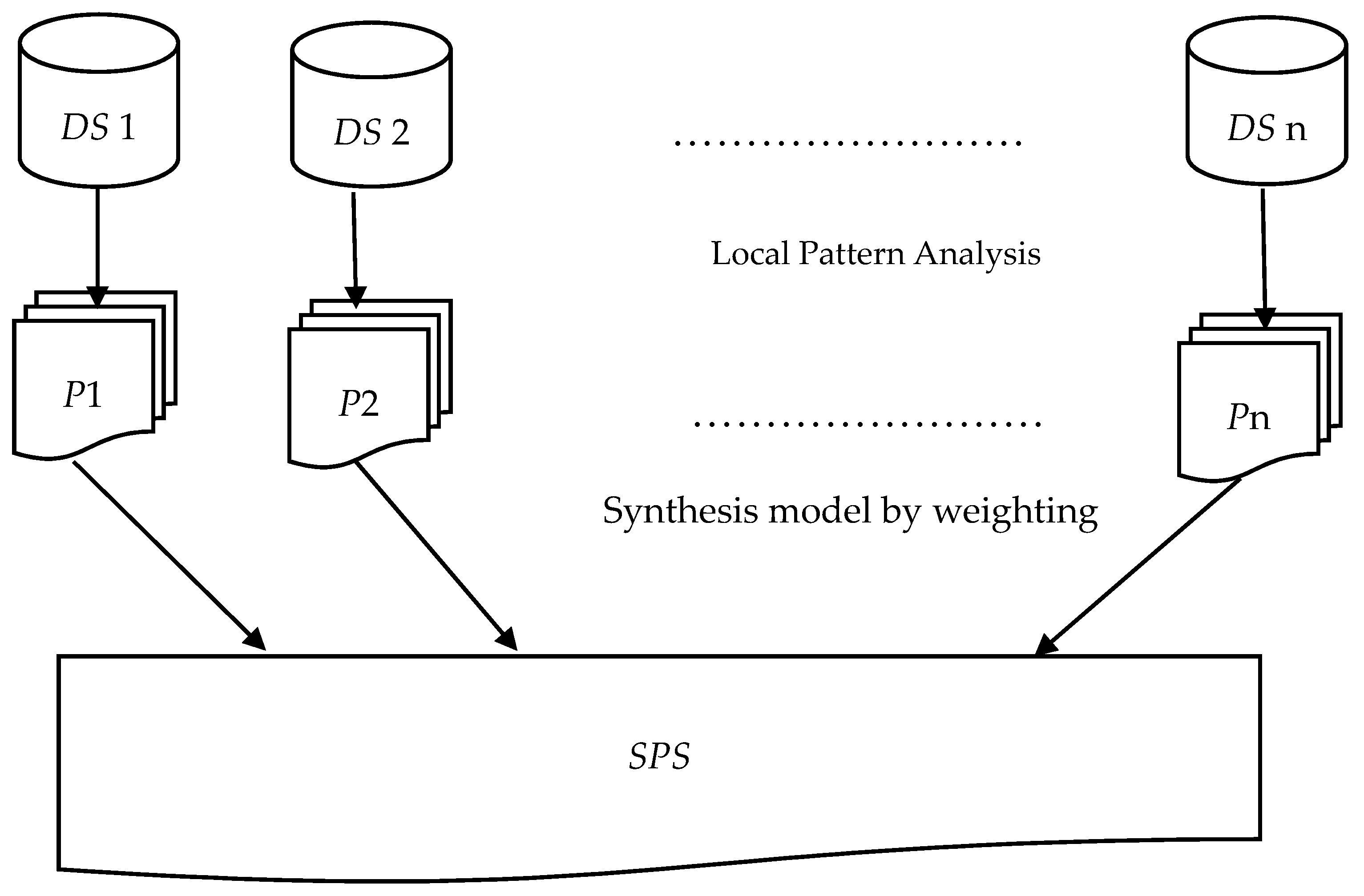
We adopt the Good’s idea [26] based on the weight of evidence for allocating weights to our data sources as the same was also adopted by Wu’s proposed model [17]. It establishes that the weight of evidence is as important as the probability itself. For convenience, we normalize the weights in the interval 0–1 and the weight of each pattern is important, based on its presence in the original database. Therefore, we use the presence of patterns to evaluate the weight of the pattern. Figure 1 outlines the proposed method. Our weighted model is designed in following sections with an example. Pattern selection algorithm is constructed to deal with low-utility patterns.
3.1. Allocating Weights to Patterns
The weight of each data source needs to be calculated in order to synthesize the high-utility patterns forwarded by different and known data sources. Let P be the set of patterns forwarded by n different data sources DS1, DS2, DS3, …, DSn and P = P1 ∪ P2 ∪ P3 ∪ … ∪ Pn where Pi is the set of patterns forwarded by DSi. According to Good’s idea of allocating weight, we take the number of occurrences of Pattern R in P to assign weight W(R) to R. High-utility patterns have higher chances of becoming a valid pattern than low-utility patterns, in the combination of all the data sources. Thus, the weight of a pattern depends upon the number of data sources that support/vote for it. In reality, a business organization is interested in mining patterns voted by most of its branches for generating maximum profit. The weight of data source also depends upon the number of high-utility patterns it supports. The following example illustrates this idea:
- Let P1 be the set of patterns mined from DS1 having patterns: ABC, AD and BE where util1(ABC) = 3,544,830; util1(AD) = 1,728,899; util1(BE) = 1,464,888
- Let P2 be the set of patterns mined from DS2 having patterns: ABC and AD where util2(ABC) = 3,591,954; util2(AD) = 1,745,716
- Let P3 be the set of patterns mined from DS3 having patterns: BC, AD and BE where util3(BC) = 1,252,220; util3(AD) = 1,749,528; util3(BE) = 1,461,862
If there are 3 data sources viz., DS1, DS2, DS3 then P = P1 ∪ P2 ∪ P3 having four patterns in P:
- R1: ABC; Number of occurrences = 2
- R2: AD; Number of occurrences = 3
- R3: BE; Number of occurrences = 2
- R4: BC; Number of occurrences = 1
We assume that the minimum utility threshold (minutil) is set to 800,000 for running example and the minimum voting degree, µ = 0.4 (Number of occurrences in P/Number of total data sources) in the pattern selection algorithm. Hence, the patterns selected are:
- µ(R1) = 2/3 = 0.6 > µ (keep)
- µ(R2) = 3/3 = 1 > µ (keep)
- µ(R3) = 2/3 = 0.6 > µ (keep)
- µ(R4) = 1/3 = 0.3 < µ (wiped out)
Pattern R1 is voted by 2 data sources, pattern R2 is voted by all 3 data sources, pattern R3 is voted by 2 sources and pattern R4 is voted by only 1 data source so it is wiped out in pattern selection procedure. To assign the weights to patterns, we use Good’s weighted model, that is, the number of occurrences of a pattern in P is used to define the weight of the pattern. The weights of patterns are assigned as:
- W(R1) = 2/(2 + 3 + 2) = 0.29
- W(R2) = 3/(2 + 3 + 2) = 0.42
- W(R3) = 2/(2 + 3 + 2) = 0.29
For n different data sources, we have P = P1 ∪ P2 ∪ P3 ∪, …, ∪ Pn and P contains R1, R2, R3,…, Rm patterns. Hence, the weight of any pattern Ri can be given as:
where j = 1, 2, 3, …, n and Occurrence(Ri) = Number of occurrences of pattern Ri in P.
W(Ri) = Occurrence(Ri)/∑ Occurrence (Rj)
3.2. Allocating Weights to Data Sources
Here, it is clearly seen that weight of data source is directly proportional to the weight of patterns mined by it. The weight of the data sources is assigned as:
- W(DS1) = (2 × 0.29) + (3 × 0.42) + (2 × 0.29) = 2.42
- W(DS2) = (2 × 0.29) + (3 × 0.42) = 1.84
- W(DS3) = (2 × 0.29) + (3 × 0.42) = 1.84
Since the values are exceeding beyond the range, we normalize and reassign the weights as:
- W(DS1) = 2.42/(2.42+1.84+1.84) = 0.396
- W(DS2) = 1.84/(2.42+1.84+1.84) = 0.302
- W(DS3) = 1.84/(2.42+1.84+1.84) = 0.302
Data source DS1 has the highest weight since it votes most patterns with high-utility and data source DS2 has the lowest weight since it votes least patterns with high-utility. For n different data sources, we have P = P1 ∪ P2 ∪ P3 ∪ … ∪ Pn and P contains R1, R2, R3, …, Rm patterns. Hence, the weight of any data source DSi can be given as:
where, i = 1, 2, 3, …, n; j = 1, 2, 3, …, n; Rx i; Ry Pj.
W(DSi) = ∑ Occurrence(Rx) × W(Rx)/∑ ∑ Occurrence(Ry) × W(Ry)
3.3. Synthesizing the Utility of Patterns
We can synthesize the utility patterns after all the different data sources are assigned weights. The synthesizing process of patterns is demonstrated below:
- Pattern R1: ABCutil(ABC) = [W(DS1) × util1(ABC)] + [W(DS2) × util2(ABC)] = [0.396 × 3,544,830] +
[0.302 × 3,591,954] = 2,488,523 - Pattern R2: ADutil(AD) = [W(DS1) × util1(AD)] + [W(DS2) × util2(AD)] + [W(DS3) × util3(AD)] =
[0.396 × 1,728,899] + [0.302 × 1,745,716] + [0.302 × 1,749,528] = 1,740,208 - Pattern R3: BEutil(BE) = [W(DS1) × util1(BE)] + [W(DS3) × util3(BE)] = [0.396 × 1,464,888] + [0.302 ×
1,461,862] = 1,021,578
All of the selected patterns satisfy the minimum threshold of utility, so they are forwarded as it is for normalizing their utility, otherwise, they are wiped out again. For n different data sources, we have P = P1 ∪ P2 ∪ P3 ∪ … ∪ Pn and P contains R1, R2, R3, …, Rm patterns. Hence, the utility of any pattern util(Ri) can be calculated as:
util(Ri) = ∑ W(DSi) × utili(Ri)
3.4. Normalizing the Utility of Patterns
The synthesized utility obtained after allocating the weights can be in the larger range depending upon the utilities specified for an item in the transaction database. According to Good’s idea, this synthesized utility can be normalized in the interval 0–1 for our simplicity. To calculate the normalized utility, the maximum profit generated in that transaction database and the number of occurrences of the pattern are used. The maximum profit generated by any item(s) after mining the union of DS1, DS2 and DS3, is 17,824,032. Hence, this value is used as Maximum_Profit while normalizing the utility of patterns. The normalization of synthesized utility is demonstrated:
- Pattern R1: ABCNutil(ABC) = (2,488,523 × 2)/17,824,032 = 0.28
- Pattern R2: ADNutil(AD) = (1,740,208 × 3)/17,824,032 = 0.293
- Pattern R3: BENutil(BE) = (1,021,578 × 2)/17,824,032 = 0.115
From the above results, the ranking of patterns is R2 (nutil = 0.293), R1(nutil = 0.28) and R3 (nutil = 0.115). For n different data sources, we have P = P1 ∪ P2 ∪ P3 ∪…∪ Pn and P contains R1, R2, R3, …, Rm patterns. Hence the normalized utility for any pattern Ri Can be given as:
Nutil(Ri) = [util(Ri) × Occurrence(Ri)]/Maximum_Profit
4. Algorithm Design
When we combine all of the high-utility patterns from different data sources, it can amass a huge number of patterns overall. To deal with this problem, we first design a pattern selection algorithm for selecting only those patterns occurring more than the number of times specified by the user, that is, by specifying a minimum voting degree, µ. The minimum voting degree, µ is a user-specified value in the range 0–1. For example, if we want only those patterns whose occurrence is in more than 60% of data sources then µ is set to be 0.6. This algorithm only enhances our synthesis model by wiping out patterns whose occurrences is below the threshold µ. The patterns having a smaller number of occurrences are seen as noise and considered to be irrelevant in the set of all patterns. These irrelevant patterns are removed before assigning weights to data sources. The output of this algorithm will be a set of filtered patterns. We design a pattern selection algorithm as Algorithm 1 below:
| Algorithm 1: Pattern_Selection (P): |
| Input: P-Set of ‘N’ patterns forwarded by different data sources; n—Number of different sources; µ—Minimum voting degree. Output: The filtered set of patterns P. 1. for i = 1 to N do a. Occurrence(Ri) = Number of occurrences of Ri in P; b. if (Occurrence(Ri)/n < µ) i. P = P − {Ri}; 2. end for; 3. return P; |
Let DS1, DS2, DS3, …, DSn be n different data sources, generating the universal set of patterns P = P1 ∪ P2 ∪ P3 ∪ … ∪ Pn where P is the set of patterns forwarded by DSi (i = 1, 2, 3, …, n). utili(Rj) is the utility of pattern Rj in DSi. minutil and Maximum_Profit are the thresholds set by the user. We design the following Algorithm 2 for synthesizing patterns from different data sources:
| Algorithm 2: Pattern_Synthesis (): |
| Input: Pattern sets P1, P2, P3, …, Pn; minimum utility threshold-minutil; Maximum_Profit. Output: Synthesized patterns with their utility. 1. Combine all sets P1, P2, P3, …, Pn into P by assigning Pattern ID to each distinguished pattern. 2. call Pattern_Selection(P); 3. for Ri P do a. Occurrence(Ri) = Number of occurrences of Ri in P; b. W(Ri) = Occurrence(Ri)/∑Occurrence(Rj P); 4. for i = 1 to n do a. W(DSi) = ∑ Occurrence(Rx Pi) × W(Rx)/∑ ∑ Occurrence(Ry Pj) × W(Ry); j = 1, 2, 3, …, n. 5. for Ri P do a. util(Ri) = ∑ W(DSi) × utili(Ri); b. if(util(Ri) < minutil) i. P = P − {Ri}; c. else i. Nutil(Ri) = [util(Ri) × Occurrence(Ri)]/Maximum_Profit; 6. sort all the patterns in P by their normalized utility i.e., Nutil(Ri); 7. return all the rules ranked by their Nutil(Ri); end. |
The above pattern synthesis algorithm synthesizes high-utility patterns ranked by their normalized utility. Step 1 combines all the sets of patterns forwarded by different data sources and assigns a unique pattern ID. Step 2 calls the algorithm Pattern_Selection (Algorithm 1) for removing the patterns occurring below the threshold µ. Step 3 assigns the weights to all patterns. Step 4 assigns the weight to all data sources. Step 5 calculates the synthesized utility and normalized utility of selected patterns. Steps 6 and 7 returns the synthesized patterns with their rank wise utility.
5. Data Description
The mining algorithms were used from SPMF Open-Source Data Mining Library [27] for performing mining through various datasets. We used Microsoft Excel for calculations and data visualization. All of the datasets used were taken from the same SPMF library. The transactions in the datasets are already having the internal utility and profit per item, hence there is no need to assign any kind of utility factor to any item. We evaluate the effectiveness of the proposed synthesis model by extensively experimenting with the datasets with varied characteristics.
6. Experimental Evaluation
The pattern ID denotes the number given to each itemset in the transaction database. The itemset shows the items appearing together in a pattern. The deviation measure between the proposed method and mono-mining is calculated by following formula:
where Nutili MM = Util(Ri) in the union of all the databases/Maximum_Profit of the database and Nutil i SM is the synthesized utility calculated by the proposed model.
Deviation = | Nutili MM − Nutili SM |
6.1. Study 1
Kosarak is a very sparse dataset containing 990,000 sequences of click-stream data from a Hungarian news portal, having 41,270 distinct items. It is partitioned into 5 databases with 198,000 transactions each, representing 5 different data sources. We first performed mono-mining on the union of these 5 databases using the D2HUP algorithm [28] and calculated the normalized utility denoted by Nutili MM. Then we mined these 5 databases separately by using the D2HUP algorithm and then applied our synthesis model to calculate normalized utility denoted by Nutili SM when minutil = 800,000, µ = 0.4, Maximum_Profit = 17,824,032. The average deviation was found to be 0.001 for two different methods. The patterns mined from different databases and ranked with its synthesized utility are tabulated in Table 3.
6.2. Study 2
Chainstore is a very sparse dataset containing 1,112,949 sequences of customer transactions from a retail store, obtained and transformed from NU-Mine Bench, having 46,086 distinct items. It is partitioned into 5 databases with 222,589 transactions each, representing 5 different data sources. We first performed mono-mining on the union of these 5 databases by D2HUP algorithm [28] and calculated the normalized utility denoted by Nutili MM. Then we mined these 5 databases separately by using the D2HUP algorithm and then applied our synthesis model to calculate normalized utility denoted by Nutili SM when minutil = 500,000, µ = 0.6, Maximum_Profit = 82,362,000. The average deviation was found to be 0.004 for two different methods. The patterns mined from different databases and ranked with its synthesized utility are tabulated in Table 4.
6.3. Study 3
Retail is a sparse dataset containing 88,162 sequences of anonymous retail market basket data from an anonymous Belgian retail store, having 16,470 distinct items. It is partitioned into 4 databases with 22,040 transactions each, representing 4 different data sources. We first performed mono-mining on the union of these 4 databases using the EFIM algorithm [20] and calculated the normalized utility denoted by Nutili MM. Then we mined these 4 databases separately by using the EFIM algorithm, and then applied our synthesis model to calculate normalized utility denoted by Nutili SM when minutil = 20,000, µ = 0.75, Maximum_Profit = 481,021. The average deviation was found to be 0.025 for two different methods. The patterns mined from different databases and ranked with its synthesized utility are tabulated in Table 5.
6.4. Study 4
BMS is a sparse dataset containing 59,601 sequences of clickstream data from an e-commerce having 497 distinct items. It is partitioned into 3 databases with 19,867 transactions each, representing 3 different data sources. We first performed mono-mining on the union of these 3 databases using the EFIM algorithm [20] and calculated the normalized utility denoted by Nutili MM. Then we mined these 3 databases separately by using the EFIM algorithm, and then applied our synthesis model to calculate normalized utility denoted by Nutili SM when minutil = 500,000, µ = 0.3, Maximum_Profit = 9,449,280. The average deviation was found to be 0.032 for the two different methods. The patterns mined from different databases and ranked with its synthesized utility are tabulated in Table 6.
6.5. Study 5
Foodmart 1 is a sparse dataset containing 4591 sequences of customer transactions from a retail store, obtained and transformed from the SQL-Server 2000, having 1559 distinct items. It is partitioned into 3 databases with 1530 transactions each, representing 3 different data sources. We first performed mono-mining on the union of these 3 databases using the EFIM algorithm [20] and calculated the normalized utility denoted by Nutili MM. Then we mined these 3 databases separately by using the EFIM algorithm and then applied our synthesis model to calculate normalized utility denoted by Nutili SM when minutil = 9000, µ = 0.3, Maximum_Profit = 30,240. The average deviation was found to be 0.524 for two different methods. The patterns mined from different databases and ranked with its synthesized utility are tabulated in Table 7.
6.6. Study 6
Foodmart 2 is a sparse dataset containing 9233 sequences of customer transactions from a retail store, obtained and transformed from the SQL-Server 2000, having 1559 distinct items. It is partitioned into 3 databases with 1530 transactions each, representing 3 different data sources. We first performed mono-mining on the union of these 3 databases using the EFIM algorithm [20] and calculated the normalized utility denoted by Nutili MM. Then we mined these 3 databases separately by using the EFIM algorithm and then applied our synthesis model to calculate normalized utility denoted by Nutili SM when minutil = 20,000, µ = 0.6, Maximum_Profit = 71,355. The average deviation was found to be 0.301 for the two different methods. The patterns mined from different databases and ranked with its synthesized utility are tabulated in Table 8.
6.7. Study 7
Accident is a moderately dense dataset containing 340,183 sequences of anonymized traffic accident data having 468 distinct items. It is partitioned into 4 databases with 85,045 transactions each, representing 4 different data sources. We first performed mono-mining on the union of these 4 databases using the EFIM algorithm [20] and calculated the normalized utility denoted by Nutili MM. Then we mined these 4 databases separately by using the EFIM algorithm, and then applied our synthesis model to calculate normalized utility denoted by Nutili SM when minutil = 7,500,000, µ = 0.5, Maximum_Profit = 31,171,329. The average deviation was found to be 0.101 for the two different methods. The patterns mined from different databases and ranked with its synthesized utility are tabulated in Table 9.
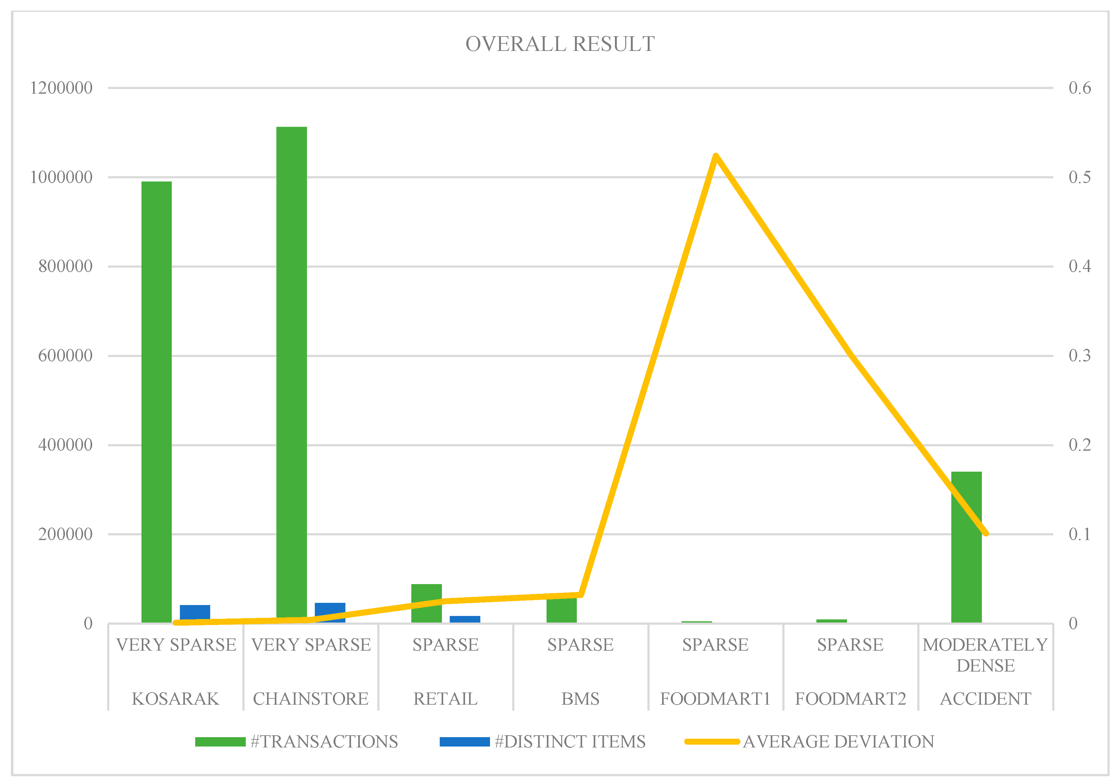
6.8. Result Analysis
Table 10 summarizes the characteristics of datasets used along with the deviations found in both methods. The average deviation for each dataset is calculated by following formula:
where N = Number of patterns forwarded by n data sources; Nutili MM, Nutili SM are calculated as per the algorithm designed.
Average Deviation = ∑ (| Nutili MM − Nutili SM |)/N
The top k patterns mined by both the methods are almost identical in each dataset, hence the proposed model is able to mine and synthesize the high-utility patterns from different databases. The proposed model worked very well for very sparse and sparse datasets having a huge number of transactions under the study. However, it is difficult to find common patterns from multiple sources for the dense datasets, especially when the number of transactions and distinct items under study are very low (or high). Hence, only one dense dataset is considered here. The different datasets used were partitioned and mined to be treated as multiple databases, after which they have applied the proposed synthesis model. Figure 2 depicts the visualization of results found. The average deviation increases as the density of databases increases, but this trend is reversed for the Accident dataset. This is due to the presence of the high number of transactions in that dataset. So, the average deviation also depends upon the number of transactions.
6.9. Runtime Performance
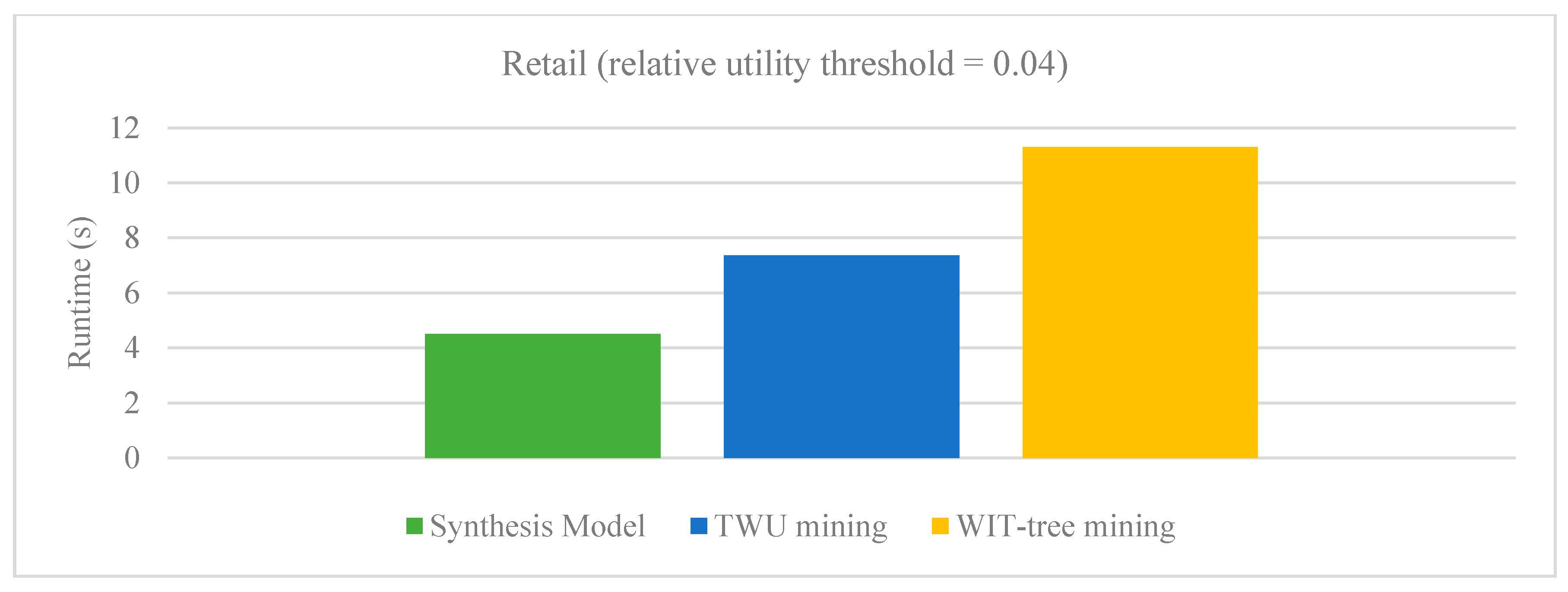
There are very few approaches proposed for aggregating high-utility patterns from multiple databases. Various known techniques such as sampling, distributed and parallel algorithms are proposed. However, the sampling technique depends heavily on the transactions of the databases which are randomly appended into a database to hold the property of binomial distribution. The limitations of parallel mining algorithms which require hardware technology are already discussed in previous sections. The runtime performance of our proposed synthesis model is evaluated with PHUI-Miner, sampling approach developed by Chen et al. [29] and parallel mining method developed by Vo et al. [30]. Figure 3 and Figure 4 respectively show the results of our Synthesis model with sampling algorithms PHUI-Miner and PHUI-MinerRnd on Kosarak and Accident dataset. In the figures we can observe that our Synthesis model (SM) clearly outperforms the PHUI-Miner and PHUI-MinerRnd algorithms on both the datasets. Figure 5 and Figure 6 respectively show the results of our Synthesis model with Vo’s model on BMS and Retail dataset. The relative utility threshold for our proposed model is the ratio of minutil to Maximum_Profit. In the figures we can observe that our Synthesis model (SM) clearly outperforms the Vo’s model on both the datasets. The reason that these datasets were selected for comparison is that only these are common in all the studies.
7. Conclusions
This paper provides an extension to the work of Wu’s model which is only applicable to frequent patterns, whereas our approach is applicable to frequent patterns as well as high-utility patterns in multiple databases. Experiments conducted in this study show that the results of the synthesis model and mono-mining are almost identical, hence the goal set during problem formation has been achieved.
The proposed method is useful when data sources are widely distributed and are not desirable to transport their whole database at the central node. The local pattern analysis gives the insights of the local behavior of nodes, whereas the global pattern analysis gives the insights of global behavior of nodes. The local analysis is useful for studying patterns at the local level and also at the global level, depending upon the weight of the local source in a global scenario. The weights of sources give the importance of local sources. However, the reliability of the weighted model proposed in this paper is an important issue to be discussed. If a given pattern occurs only in a single data source, if its synthesized utility is well above the threshold then it has to be considered as a high-utility valid pattern. Arbitrarily requiring that a pattern has to occur in multiple sources is not justified. There could be interaction effects between the parameters of different sources and they should also be considered in the equations defined.
Our proposed approach in this paper is suitable when data comes from different sources, such as sensor networks in the Internet of Things (IoT). Our approach is also beneficial when store managers are interested in high-profit items. This work can be extended further for dense datasets, as the results found for them were not very effective. Our future work will also focus on synthesizing patterns with negative utility, on-shelf with negative profit units and high-utility sequential rule/pattern mining.
Author Contributions
conceptualization, A.M. and M.G.; methodology, A.M.; formal analysis, A.M.; writing—original draft preparation, A.M.; writing—review and editing, A.M.; visualization, A.M.; supervision, M.G.
Funding
This research received no external funding.
Acknowledgments
We acknowledge the support given by the Department of Computer Engineering, SVPCET, Nagpur, India for carrying out this research.
Conflicts of Interest
The authors declare no conflict of interest.
References
- Pujari, A. Data Mining Techniques; Universities Press (India) Private Limited: Hyderabad, India, 2013. [Google Scholar]
- Marr, B. Really Big Data at Walmart Real Time Insights from Their 40-Petabyte Data Cloud. Available online: www.forbes.com/sites/bernardmarr/2017/01/23/really-big-data-at-walmart-real-time-insights-from-their-40-petabyte-data-cloud/ (accessed on 21 August 2018).
- Taste of Efficiency: How Swiggy Is Disrupting Food Delivery with ML, AI. Available online: https://www.financialexpress.com/industry/taste-of-efficiency-how-swiggy-is-disrupting-food-delivery-with-ml-ai/1288840/ (accessed on 23 August 2018).
- Agrawal, R.; Shafer, J.C. Parallel mining of association rules. IEEE Trans. Knowl. Data Eng. 1996, 8, 962–969. [Google Scholar] [CrossRef] [Green Version]
- Chattratichat, J.; Darlington, J.; Ghanem, M.; Guo, Y.; Hüning, H.F.; Köhler, M.; Yang, D. Large Scale Data Mining: Challenges and Responses. In Proceedings of the Third International Conference on Knowledge Discovery and Data Mining (KDD-97), Newport Beach, CA, USA, 14–17 August 1997; pp. 143–146. [Google Scholar]
- Cheung, D.W.; Han, J.; Ng, V.T.; Wong, C.Y. Maintenance of discovered association rules in large databases: An incremental updating technique. In Proceedings of the Twelfth International Conference on Data Engineering, New Orleans, LA, USA, 26 Feburaury–1 March 1996; pp. 106–114. [Google Scholar]
- Parthasarathy, S.; Zaki, M.J.; Ogihara, M.; Li, W. Parallel data mining for association rules on shared-memory systems. Knowl. Inf. Syst. 2001, 3, 1–29. [Google Scholar] [CrossRef]
- Shintani, T.; Kitsuregawa, M. Parallel mining algorithms for generalized association rules with classification hierarchy. In Proceedings of the 1998 ACM SIGMOD International Conference on Management of Data, Seattle, WA, USA, 1–4 June 1998; pp. 25–36. [Google Scholar]
- Xun, Y.; Zhang, J.; Qin, X. Fidoop: Parallel mining of frequent itemsets using mapreduce. IEEE Trans. Syst. Man Cybern. Syst. 2016, 46, 313–325. [Google Scholar] [CrossRef]
- Zhang, F.; Liu, M.; Gui, F.; Shen, W.; Shami, A.; Ma, Y. A distributed frequent itemset mining algorithm using Spark for Big Data analytics. Clust. Comput. 2015, 18, 1493–1501. [Google Scholar] [CrossRef]
- Marjani, M.; Nasaruddin, F.; Gani, A.; Karim, A.; Hashem, I.A.T.; Siddiqa, A.; Yaqoob, I. Big IoT data analytics: architecture, opportunities, and open research challenges. IEEE Access 2017, 5, 5247–5261. [Google Scholar]
- Wang, R.; Ji, W.; Liu, M.; Wang, X.; Weng, J.; Deng, S.; Gao, S.; Yuan, C. Review on mining data from multiple data sources. Pattern Recognit. Lett. 2018, 109, 120–128. [Google Scholar] [CrossRef]
- Adhikari, A.; Adhikari, J. Mining Patterns of Select Items in Different Data Sources; Springer: Cham, Switzerland, 2014. [Google Scholar]
- Lin, Y.; Chen, H.; Lin, G.; Chen, J.; Ma, Z.; Li, J. Synthesizing decision rules from multiple information sources: A neighborhood granulation viewpoint. Int. J. Mach. Learn. Cybern. 2018, 9, 1–10. [Google Scholar] [CrossRef]
- Zhang, S.; Wu, X.; Zhang, C. Multi-database mining. IEEE Comput. Intell. Bull. 2003, 2, 5–13. [Google Scholar]
- Xu, W.; Yu, J. A novel approach to information fusion in multi-source datasets: A granular computing viewpoint. Inf. Sci. 2017, 378, 410–423. [Google Scholar] [CrossRef]
- Wu, X.; Zhang, S. Synthesizing high-frequency rules from different data sources. IEEE Trans. Knowl. Data Eng. 2003, 15, 353–367. [Google Scholar] [Green Version]
- Ramkumar, T.; Srinivasan, R. Modified algorithms for synthesizing high-frequency rules from different data sources. Knowl. Inf. Syst. 2008, 17, 313–334. [Google Scholar] [CrossRef]
- Savasere, A.; Omiecinski, E.R.; Navathe, S.B. An efficient algorithm for mining association rules in large databases. In Proceedings of the 21th International Conference on Very Large Data Bases, San Francisco, CA, USA, 11–15 September 1995; pp. 432–444. [Google Scholar]
- Zida, S.; Fournier-Viger, P.; Lin, J.C.W.; Wu, C.W.; Tseng, V.S. EFIM: a fast and memory efficient algorithm for high-utility itemset mining. Knowl. Inf. Syst. 2017, 51, 595–625. [Google Scholar] [CrossRef]
- Liu, Y.; Liao, W.K.; Choudhary, A. A fast high-utility itemsets mining algorithm. In Proceedings of the 1st International Workshop on Utility-Based Data Mining, Chicago, IL, USA, 21 August 2005; pp. 90–99. [Google Scholar]
- Agrawal, R.; Imieliński, T.; Swami, A. Mining association rules between sets of items in large databases. In Proceedings of the 1993 ACM SIGMOD International Conference on Management of Data, Washington, DC, USA, 25–28 May 1993; pp. 207–216. [Google Scholar]
- Yao, H.; Hamilton, H.J.; Geng, L. A unified framework for utility-based measures for mining itemsets. In Proceedings of the ACM SIGKDD 2nd Workshop on Utility-Based Data Mining, Philadelphia, PA, USA, 20–23 August 2006; pp. 28–37. [Google Scholar]
- Ahmed, C.F.; Tanbeer, S.K.; Jeong, B.S.; Lee, Y.K. Efficient tree structures for high-utility pattern mining in incremental databases. IEEE Trans. Knowl. Data Eng. 2009, 21, 1708–1721. [Google Scholar] [CrossRef]
- Fournier-Viger, P.; Wu, C.W.; Tseng, V.S. Novel Concise Representations of High-Utility Itemsets Using Generator Patterns. In Advanced Data Mining and Applications; Luo, X., Yu, J.X., Li, Z., Eds.; Springer: Cham, Switzerland, 2014; Volume 8933, pp. 30–43. [Google Scholar]
- Good, I.J. Probability and the Weighting of Evidence; Charles Griffin: Madison, WI, USA, 2007. [Google Scholar]
- Fournier-Viger, P.; Lin, C.W.; Gomariz, A.; Gueniche, T.; Soltani, A.; Deng, Z.; Lam, H.T. The SPMF Open-Source Data Mining Library Version 2. In Proceedings of the 19th European Conference on Principles of Data Mining and Knowledge Discovery (PKDD 2016) Part III, Riva del Garda, Italy, 19–23 September 2016; pp. 36–40. [Google Scholar]
- Liu, J.; Wang, K.; Fung, B.C. Mining high-utility patterns in one phase without generating candidates. IEEE Trans. Knowl. Data Eng. 2016, 28, 1245–1257. [Google Scholar] [CrossRef]
- Chen, Y.; An, A. Approximate parallel high-utility itemset mining. Big Data Res. 2016, 6, 26–42. [Google Scholar] [CrossRef]
- Vo, B.; Nguyen, H.; Ho, T.B.; Le, B. Parallel Method for Mining High-Utility Itemsets from Vertically Partitioned Distributed Databases. In Knowledge-Based and Intelligent Information and Engineering Systems. KES 2009. Lecture Notes in Computer Science; Velásquez, J.D., Ríos, S.A., Howlett, R.J., Jain, L.C., Eds.; Springer: Berlin, Germany, 2009; Volume 5711, pp. 251–260. [Google Scholar]
Figure 1.
The proposed model of synthesizing patterns by weighting. DS i—ith data source; P i—Pattern set mined from DS i; SPS—The synthesized pattern set with normalized utility.
Figure 1.
The proposed model of synthesizing patterns by weighting. DS i—ith data source; P i—Pattern set mined from DS i; SPS—The synthesized pattern set with normalized utility.

Figure 2.
Data visualization for overall results.

Figure 3.
Running time on Kosarak dataset.

Figure 4.
Running time on Accident dataset.
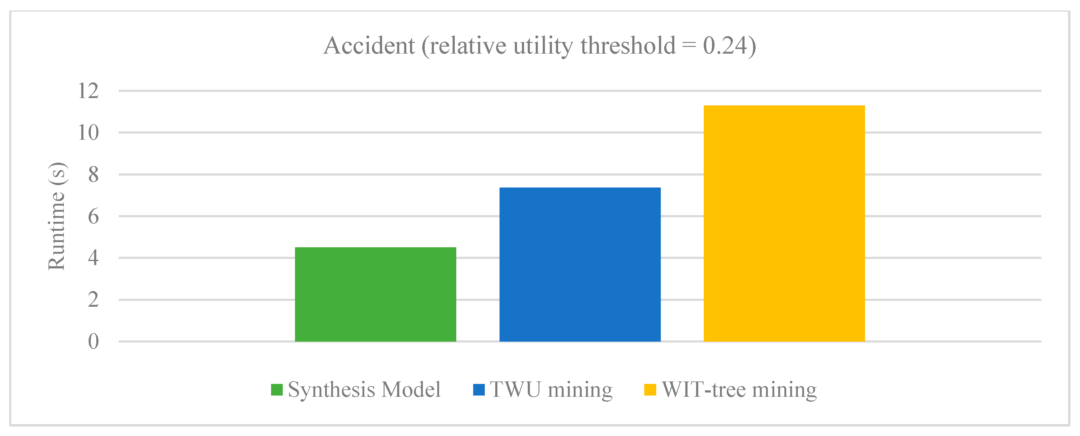
Figure 5.
Running time on BMS dataset.
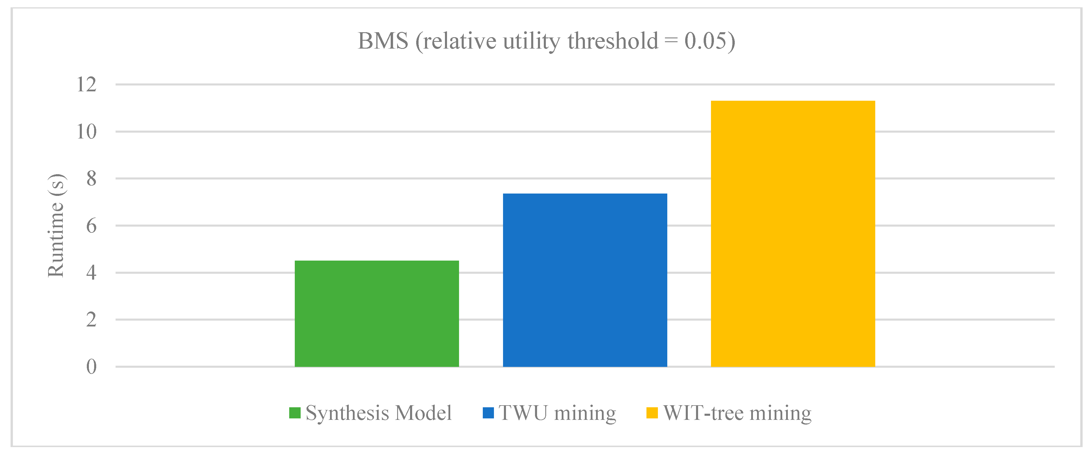
Figure 6.
Running time on Retail dataset.

Table 1.
Sample transaction database.
| TID | Transaction (Item, Quantity) |
|---|---|
| T1 | (p, 2), (r, 3), (s, 5) |
| T2 | (p, 3), (r, 7), (t, 3), (v, 6) |
| T3 | (p, 2), (q, 3), (r, 2), (s, 7), (t, 2), (u, 6) |
| T4 | (q, 5), (r, 4), (s, 4), (t, 2) |
| T5 | (q, 3), (r, 3), (t, 2), (v, 3) |
Table 2.
External utility.
| Item | p | q | r | s | t | u | v |
|---|---|---|---|---|---|---|---|
| Profit | 6 | 3 | 2 | 3 | 4 | 2 | 2 |
Table 3.
Experimental results for Kosarak dataset.
| Pattern ID | Itemset | NutiliMM | NutiliSM | Deviation |
|---|---|---|---|---|
| P1 | 11, 6 | 1 | 0.999 | 0.001 |
| P2 | 3, 11, 6 | 0.488 | 0.487 | 0.001 |
| P3 | 3, 6 | 0.41 | 0.409 | 0.001 |
| P4 | 3, 11 | 0.348 | 0.348 | 0.000 |
| P6 | 1, 11, 6 | 0.293 | 0.292 | 0.001 |
| P5 | 148, 218, 11, 6 | 0.293 | 0.291 | 0.002 |
| P7 | 148, 11, 6 | 0.29 | 0.290 | 0.000 |
| P8 | 148, 218, 11 | 0.232 | 0.232 | 0.000 |
| P9 | 148, 218, 6 | 0.228 | 0.228 | 0.000 |
Table 4.
Experimental results for Chainstore dataset.
| Pattern ID | Itemset | NutiliMM | NutiliSM | Deviation |
|---|---|---|---|---|
| P1 | 39,171, 39,688 | 0.078 | 0.077 | 0.001 |
| P5 | 39,692, 39,690 | 0.062 | 0.063 | 0.001 |
| P4 | 5166, 16,967 | 0.051 | 0.052 | 0.001 |
| P3 | 21,283, 21,308 | 0.05 | 0.051 | 0.001 |
| P6 | 16,977, 16,967 | 0.05 | 0.051 | 0.001 |
| P9 | 22,900, 21,308 | 0.049 | 0.049 | 0.000 |
| P7 | 39,206, 39,182 | 0.055 | 0.044 | 0.011 |
| P8 | 10,481, 16,967 | 0.042 | 0.042 | 0.000 |
| P2 | 39,143, 39,182 | 0.052 | 0.029 | 0.023 |
Table 5.
Experimental results for the Retail dataset.
| Pattern ID | Itemset | NutiliMM | NutiliSM | Deviation |
|---|---|---|---|---|
| P1 | 49, 40 | 1 | 1 | 0.000 |
| P2 | 49 | 0.963 | 0.964 | 0.001 |
| P7 | 40 | 0.579 | 0.579 | 0.000 |
| P8 | 33 | 0.523 | 0.524 | 0.001 |
| P9 | 33, 49 | 0.461 | 0.463 | 0.002 |
| P3 | 42, 40 | 0.522 | 0.422 | 0.100 |
| P5 | 42, 49 | 0.516 | 0.418 | 0.098 |
| P4 | 42 | 0.513 | 0.416 | 0.097 |
| P6 | 42, 49, 40 | 0.506 | 0.409 | 0.097 |
| P10 | 33, 40 | 0.387 | 0.388 | 0.001 |
| P12 | 33, 49, 40 | 0.372 | 0.373 | 0.001 |
| P17 | 39, 49 | 0.363 | 0.363 | 0.000 |
| P14 | 39 | 0.353 | 0.353 | 0.000 |
| P16 | 39, 40 | 0.353 | 0.353 | 0.000 |
| P20 | 39, 49, 40 | 0.349 | 0.349 | 0.000 |
| P19 | 37, 39 | 0.317 | 0.327 | 0.010 |
| P25 | 37 | 0.268 | 0.266 | 0.002 |
| P27 | 37, 39, 40 | 0.243 | 0.242 | 0.001 |
| P26 | 171, 39 | 0.207 | 0.208 | 0.001 |
| P28 | 37, 40 | 0.209 | 0.208 | 0.001 |
| P30 | 37, 39, 49 | 0.186 | 0.184 | 0.002 |
| P13 | 39, 42 | 0.224 | 0.182 | 0.042 |
| P11 | 33, 42 | 0.219 | 0.177 | 0.042 |
| P15 | 39, 42, 40 | 0.211 | 0.171 | 0.040 |
| P22 | 39, 42, 49 | 0.191 | 0.155 | 0.036 |
| P21 | 33, 42, 49 | 0.189 | 0.153 | 0.036 |
| P18 | 33, 42, 40 | 0.187 | 0.152 | 0.035 |
| P24 | 39, 42, 49, 40 | 0.183 | 0.148 | 0.035 |
| P23 | 33, 42, 49, 40 | 0.169 | 0.137 | 0.032 |
Table 6.
Experimental results for BMS dataset.
| Pattern ID | Itemset | NutiliMM | NutiliSM | Deviation |
|---|---|---|---|---|
| P1 | 306, 315 | 0.2032 | 0.1871 | 0.016 |
| P3 | 151, 168 | 0.1768 | 0.1255 | 0.051 |
| P2 | 148, 168 | 0.1642 | 0.1250 | 0.039 |
| P5 | 306, 310 | 0.1426 | 0.1185 | 0.024 |
| P4 | 5, 168 | 0.1387 | 0.1073 | 0.031 |
Table 7.
Experimental results for the Foodmart 1 dataset.
| Pattern ID | NutiliMM | NutiliSM | Deviation |
|---|---|---|---|
| P10 | 0.901 | 0.530 | 0.371 |
| P11 | 0.848 | 0.504 | 0.344 |
| P3 | 0.845 | 0.448 | 0.397 |
| P9 | 0.836 | 0.413 | 0.423 |
| P26 | 1 | 0.220 | 0.780 |
| P12 | 0.94 | 0.188 | 0.752 |
| P1 | 0.572 | 0.165 | 0.407 |
| P13 | 0.726 | 0.155 | 0.571 |
| P2 | 0.685 | 0.148 | 0.537 |
| P14 | 0.783 | 0.140 | 0.643 |
| P4 | 0.578 | 0.137 | 0.441 |
| P5 | 0.582 | 0.135 | 0.447 |
| P6 | 0.483 | 0.132 | 0.351 |
| P15 | 0.644 | 0.132 | 0.512 |
| P7 | 0.667 | 0.131 | 0.536 |
| P16 | 0.667 | 0.127 | 0.540 |
| P8 | 0.657 | 0.124 | 0.533 |
| P17 | 0.58 | 0.121 | 0.459 |
| P20 | 0.652 | 0.116 | 0.536 |
| P21 | 0.55 | 0.116 | 0.434 |
| P23 | 0.574 | 0.113 | 0.461 |
| P38 | 0.658 | 0.075 | 0.583 |
| P39 | 0.711 | 0.074 | 0.637 |
| P40 | 0.664 | 0.073 | 0.591 |
| P41 | 0.742 | 0.072 | 0.670 |
| P43 | 0.748 | 0.071 | 0.677 |
Table 8.
Experimental results for Foodmart 2 dataset.
| Pattern ID | NutiliMM | NutiliSM | Deviation |
|---|---|---|---|
| P1 | 0.358 | 1.012 | 0.654 |
| P2 | 0.354 | 0.963 | 0.609 |
| P7 | 0.398 | 0.901 | 0.503 |
| P6 | 0.301 | 0.894 | 0.593 |
| P3 | 0.382 | 0.458 | 0.076 |
| P4 | 0.323 | 0.406 | 0.083 |
| P9 | 0.299 | 0.378 | 0.079 |
| P11 | 0.266 | 0.371 | 0.104 |
| P15 | 0.315 | 0.323 | 0.009 |
Table 9.
Experimental results for Accident dataset.
| Pattern ID | Itemset | NutiliMM | NutiliSM | Deviation |
|---|---|---|---|---|
| P2 | 28, 43 31, 16, 18, 12, 17 | 0.9913 | 0.99 | 0.001 |
| P1 | 28, 43, 21, 31, 16, 18, 12, 17 | 1 | 0.8 | 0.200 |
Table 10.
Dataset characteristics.
| Dataset | Nature of Dataset | Transactions | Distinct Items | Average Deviation |
|---|---|---|---|---|
| Kosarak | Very Sparse | 990,000 | 41,270 | 0.001 |
| Chainstore | Very Sparse | 1,112,949 | 46,086 | 0.004 |
| Retail | Sparse | 88,162 | 16,470 | 0.025 |
| BMS | Sparse | 59,601 | 497 | 0.032 |
| Foodmart1 | Sparse | 4591 | 1559 | 0.524 |
| Foodmart2 | Sparse | 9233 | 1559 | 0.301 |
| Accident | Moderately Dense | 340,183 | 468 | 0.101 |
© 2018 by the authors. Licensee MDPI, Basel, Switzerland. This article is an open access article distributed under the terms and conditions of the Creative Commons Attribution (CC BY) license (http://creativecommons.org/licenses/by/4.0/).
Share and Cite
MDPI and ACS Style
Muley, A.; Gudadhe, M. Synthesizing High-Utility Patterns from Different Data Sources. Data 2018, 3, 32. https://doi.org/10.3390/data3030032
AMA Style
Muley A, Gudadhe M. Synthesizing High-Utility Patterns from Different Data Sources. Data. 2018; 3(3):32. https://doi.org/10.3390/data3030032
Chicago/Turabian StyleMuley, Abhinav, and Manish Gudadhe. 2018. "Synthesizing High-Utility Patterns from Different Data Sources" Data 3, no. 3: 32. https://doi.org/10.3390/data3030032