GasLib—A Library of Gas Network Instances
by
 , , , , ,
Martin Schmidt
1,2,* ,
,
Denis Aßmann
1,
Robert Burlacu
1,
Jesco Humpola
3,
Imke Joormann
4,
Nikolaos Kanelakis
5,
Thorsten Koch
3,
Djamal Oucherif
6,
Marc E. Pfetsch
7,
Lars Schewe
1,2,
Robert Schwarz
3 and
Mathias Sirvent
1 1
Discrete Optimization, Friedrich-Alexander-Universität Erlangen-Nürnberg, Cauerstr. 11, 91058 Erlangen, Germany
2
Energie Campus Nürnberg, Fürther Str. 250, 90429 Nürnberg, Germany
3
Zuse Institut Berlin, Takustr. 7, 14195 Berlin, Germany
4
Institut für Mathematische Optimierung, Technische Universität Braunschweig, Universitätsplatz 2, 38106 Braunschweig, Germany
5
School of Electrical and Computer Engineering, Aristotle University of Thessaloniki, 54124 Thessaloniki, Greece
6
Institut für Angewandte Mathematik, Leibniz Universität Hannover, Welfengarten 1, 30167 Hannover, Germany
7
Department of Mathematics, Technische Universität Darmstadt, Dolivostr. 15, 64293 Darmstadt, Germany
*
Author to whom correspondence should be addressed.
Data 2017, 2(4), 40; https://doi.org/10.3390/data2040040
Submission received: 6 November 2017
/
Revised: 18 November 2017
/
Accepted: 23 November 2017
/
Published: 1 December 2017
Abstract
:The development of mathematical simulation and optimization models and algorithms for solving gas transport problems is an active field of research. In order to test and compare these models and algorithms, gas network instances together with demand data are needed. The goal of GasLib is to provide a set of publicly available gas network instances that can be used by researchers in the field of gas transport. The advantages are that researchers save time by using these instances and that different models and algorithms can be compared on the same specified test sets. The library instances are encoded in an XML (extensible markup language) format. In this paper, we explain this format and present the instances that are available in the library.
Data Set: http://gaslib.zib.de
Data Set License: CC BY 3.0
MSC:
90-08; 90C90; 90B101. Summary
The mathematical simulation and optimization of gas transport through pipeline systems is an important field of research with a large practical impact. Over the last decades, many different mathematical models on different levels of accuracy for different components of gas networks have been developed. On the basis of these models, several simulation and optimization algorithms have been proposed. We refer to [1,2,3] and the references therein for more information. With GasLib, we provide a set of network instances that can be used to test and compare such models and the algorithms for solving them.
Gas networks are used to transport gas from entry nodes, where gas is supplied, to exit nodes, where gas is discharged from the network. The set of supplied and discharged flows, together with additional specifications on the supplied and discharged gas pressures and the chemical compositions of the supplied gas, is called a nomination. In stationary models, it is typically assumed that the sum of supplied flows equals the sum of the discharged flows, that is, the nominations have to be balanced. Gas flows, except for situations with large slopes, from higher to lower pressure and the pressure drop is caused by friction at the rough inner pipe walls. This makes it necessary to increase the gas pressure in compressor stations in order to transport gas over large distances. On the other hand, gas pressure has to be reduced in control valve stations at the transition to regional distribution networks. Moreover, gas transport networks comprise other elements such as valves (e.g., to control the direction of the gas flow) or resistors (e.g., to model pressure drops caused by internal station piping or partly closed valves). We refer to Section 2.2 for the description of all network elements that are part of the GasLib networks and to the chapter [4] in the book [1] for a physical and technical description of the network elements as well as for several mathematical models.
From a mathematical point of view, the resulting problems lead to large-scale simulation instances and hard mixed-integer nonlinear and nonconvex optimization or feasibility problems. Typically, the solutions of the optimization problems are out of reach for state-of-the-art general-purpose solvers for large-scale instances. Therefore, more research is needed in order to provide accurate and fast optimization methods for practical gas transport instances. Unfortunately, gas network data is only seldom publicly available, except for the Belgian gas network data published in [5]. Moreover, the wealth of gas transport models leads to the problem that they are usually not compared or not on the same networks. The gas network library GasLib aims to fix these problems by providing publicly available small- to large-scale academic and real-world networks. It currently contains stationary instances only. The contained real-world data originates from the completed industrial research project ForNe, the project “Investigation of the technical capacities of gas networks” (2009–2012) that was funded by the German Federal Ministry of Economic Affairs and Energy, and from the collaborative research center TRR 154 “Mathematical Modelling, Simulation and Optimization using the Example of Gas Networks”, which is funded by the German Research Foundation. Because some of the original data from our former industry partner Open Grid Europe GmbH (http://www.open-grid-europe.com) and from the Greek network operator DESFA is confidential, the corresponding GasLib instances are distorted versions of the original transport networks. See Section 2.1 for a more detailed description of the instances. The complete library is freely available at http://gaslib.zib.de.
GasLib is useful for different target groups: First, researchers that develop new mathematical models and simulation or optimization algorithms can use GasLib to test and evaluate these algorithms on network instances of different sizes. Second, developers of optimization and simulation solvers can use GasLib to improve the performance and robustness of their solvers using the example of challenging models from a real-world problem.
The network instances within GasLib are composed of different data that can be used to set up simulation or optimization models for stationary gas transport problems. First, every instance includes a structural and technical description of the network and all contained network elements. Second, several sets of nominations are provided. More detailed information on the provided data and the data format is given in Section 2.2.
For some instances, GasLib additionally provides GAMS [6] models of specific mixed-integer nonlinear models based on the corresponding network instances. This collection of models can be used to test and improve solvers for mixed-integer nonlinear optimization (MINLP). The corresponding models are feasibility problems, that is, no objective function is given, as described in [1], and the modeling decisions are the same as for the MINLP model described in [7]. For instance, the MINLP instances arising from the GasLib-582 network have roughly 2200 variables (of which roughly 250 are binary) and 3700 constraints (of which roughly 900 are nonlinear). Numerical results on an earlier version of these models can be found in [2].
Finally, we like to mention that this paper does not contain descriptions of methods for solving the discussed simulation or optimization models. However, there are already some published research papers that have used GasLib instances. We give the corresponding references in Section 2.1, where we present the instances in detail.
2. Data Description
In this section, we describe the data contained in GasLib and explain the different data formats.
2.1. Overview of the Instances
GasLib currently contains seven instances: four handmade networks with 11, 24, 40, and 135 nodes intended for testing purposes, one medium-scale real-world network with 134 nodes, and two large real-world networks with 582 and 4197 nodes, respectively. In the following, we describe all the networks in detail. We note that the number of nodes is always part of the name of the network.
2.1.1. GasLib-11
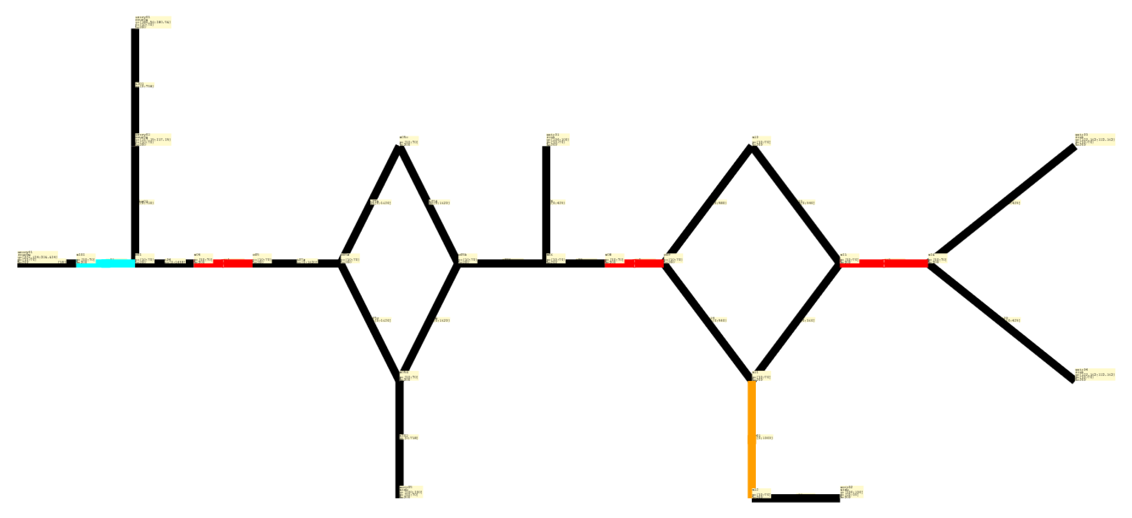
This artificial small-scale network is provided for testing purposes. Its small size allows for fast computations as well as for testing and comparing different models of network elements. The network consists of 3 entries, 3 exits, 8 pipes, 2 compressor stations, and 1 valve. It has the special property that closing the valve yields a tree-structured network topology; see Figure 1. In this and all other network plots, different colors are used to denote different network elements: black arcs are pipes or short pipes, red arcs are compressor stations, valves are green, resistors are cyan, and control valves are orange. See Section 2.2.1 for a more detailed description of these elements. The single nomination provided requires routing 300 from the entries to the exits.
2.1.2. GasLib-24
The small-scale network GasLib-24 is also provided for testing purposes. It is an extended variant of the network used in [8]; see the description in the cited paper for more details. Its small size again allows for fast computations as well as for testing and comparing different models of network elements. The network consists of 3 entries, 5 exits, 19 pipes, 3 compressor stations, and 1 control valve, short pipe, and resistor each; see Figure 2. The single nomination requires routing 544.32 units of flow from the entries to the exits. This network has already been used in the papers [9,10].
2.1.3. GasLib-40
This third small-scale network is also provided for testing purposes. Its size also allows for fast computations as well as for testing and comparing different models of network elements. The network consists of 3 entries, 29 exits, 39 pipes, and 6 compressor stations; see Figure 3. It roughly represents a part of the German low-calorific gas transport network in the Rhine-Main-Ruhr area. A single nomination is provided, in which the same amount of gas (75 ) is discharged at every exit node. The entry nodes equally provide the gas; that is, the inflow at every entry is 725 . Numerical results for this instance can be found in [11,12,13,14,15].
2.1.4. GasLib-134
The medium-scale network GasLib-134 is a close approximation of the real-world tree-like gas transport network of Greece and consists of a main pipeline connecting the Greek–Bulgarian border with southern Greece and additional 16 branches, comprising an overall length of 1412 km. The network consists of 3 entries, 45 exits, 86 inner nodes, 86 pipes, 45 short pipes, 1 turbo compressor machine, and 1 control valve with preset pressure; see Figure 4. Because of the confidential nature of the compressor’s technical data, it has been replaced by a random example that roughly approximates its main characteristics, namely, a maximum mechanical power of 7500 kW and an adiabatic efficiency of 0.84. The associated 1234 daily nominations have been taken from the transmission system operator’s website [16] and processed so that they only represent balanced samples between the entries and the exits. Moreover, all nomination data have been converted from heat power to volumetric units by utilizing a conversion with a single calorific value, thus neglecting the gas mixing within the network. This instance has been used in the papers [17,18,19].
2.1.5. GasLib-135
The medium-scale network GasLib-135 is also provided for testing purposes. It allows the testing of models on a larger network. The network consists of 6 entries, 99 exits, 30 inner nodes, 141 pipes, and 29 compressor stations. It roughly represents a part of the German high-calorific gas transport network; see Figure 5. We note that this network also contains cycles, which is not the case for the almost equally sized GasLib-134 network. This aspect typically makes the network harder to solve than GasLib-134. Again, a single nomination is provided, in which the same amount of gas (40 ) is discharged at every exit. The entries equally provide the gas; that is, the inflow at every entry is 660 . Numerical results for these instances can be found in [11,12,13,14].
2.1.6. GasLib-582
The large-scale network GasLib-582 is based on a real-world gas transport network, which covers approximately one-fourth of the area of Germany. Because the original network data from Open Grid Europe GmbH are confidential, we have carefully distorted these such that no direct conclusion regarding the true operational capability of the network can be drawn, while still maintaining a realistic behavior. In particular, the feasibility of the edited instances is comparable to that of the original instances.
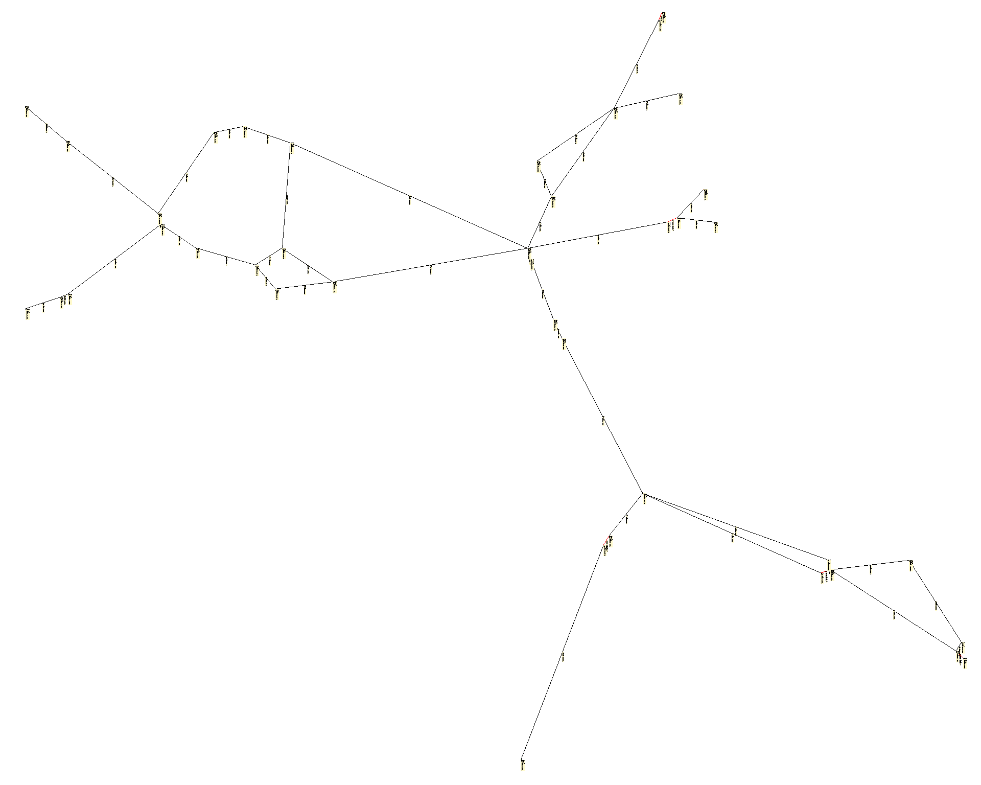
The network GasLib-582 contains 31 entries, 129 exits, and 422 inner nodes, which are connected by 278 pipes, 5 compressor stations, 23 control valves, 8 resistors, and 269 short pipes; see Figure 6. We note that this network again contains cycles. The compressor stations contain 8 turbo compressors and 1 piston compressor in total.
The associated 4227 nominations are obtained in a two-stage process. First, the load on some nodes (typically exits) are sampled from distributions that are estimated from historical data. The load for the remaining nodes is then determined such that the load is balanced and a random linear objective is maximized. See [20] for a detailed description of the entire process. Because the solution of these nominations can be rather challenging, we additionally provide a set of nominations that are scaled to 95% of the flow amount; that is, the supplied (discharged) amount of gas at every entry (exit) is scaled by 0.95.
2.1.7. GasLib-4197
The network GasLib-4197 is based on a real-world gas transport network spanning one-third of Germany. Because the original network data from Open Grid Europe GmbH again are confidential, we have carefully distorted these as described for the GasLib-582 network.
We expect the feasibility of the edited instances to be comparable to that of the original instances, but it has to be noted that given the size of the network, we are not yet able to compute feasible solutions to all scenarios. Thus, while we assume these to be feasible in reality, there is no proof for this so far.
The network contains 11 entry nodes, 1009 exit nodes, and 3177 inner nodes, as well as 3537 pipes, 12 compressor stations, 426 valves, 120 control valves, 28 resistors, and 343 short pipes; see Figure 7. The compressor stations contain 22 turbo compressors in total. The associated 2859 nominations (i.e., fixed and balanced inflow-outflow situations with pressure bounds) are obtained as sampled statistical load scenarios of the original network, similarly to GasLib-582; see [20] for a detailed description of the sampling process.
2.2. Description of the Data Files
All files contained in GasLib are XML files. XML is a language for describing data in a hierarchical format; see [27]. A multitude of software to read and write XML files on different platforms is available, rendering XML useful for collecting and publishing data that should be easy to read, to parse, and to write.
We use XSD (XML Schema Definition) files to specify the format of the XML files and the types of the data therein; see [28] for more details on XSD. The schemas given in the XSD files can be used by software to validate a given XML file against its specification or even to generate XML parsers automatically. XSD files are also written in XML.
A GasLib network is described using different files. First, the network topology itself is specified in a net file. The contained compressor machines are described in a cs file, and the interplay of different controllable elements of the network is given in a cdf file. Finally, a nomination is specified by a separate scn file. Thus, the full set for specifying a single stationary demand scenario (nomination) for a gas transport network requires four files. However, the cdf file is optional and does not need to be given. We note further that there may be arbitrarily many scn files but only one cs and one cdf file for a given network description (net) file.
Most of the data given in the mentioned files are physical or technical quantities. Thus, in order to increase the readability (both for humans and computers), every physical or technical quantity is specified by a value and a unit in which the value has to be interpreted. GasLib provides the usage of many different units for the same physical or technical quantity. Examples are given in Table 1, and a full list can be found in the documentation on the GasLib website or in the XSD files.
2.2.1. The net File
A gas network is given as a directed graph in which the nodes represent junctions and the arcs represent the elements of the network. This topology is described in the net file together with the technical parameters of the network elements.
There are three types of nodes: entry nodes (source), exit nodes (sink), and junctions (innode). Common to all types of nodes are bounds for the pressure, but source and sink nodes have additional bounds on the supplied and discharged amount of flow at the node. Positive flow at a source node refers to the injection of gas, while positive flow at a sink stands for the discharge of gas. The source nodes have additional parameters, describing the composition of the supplied gas. For example, for source nodes, we have to state the values of, for example, the calorific value or the pseudocritical temperature; see Figure 8. The flow bounds at the nodes in the net file are usually very wide. Fixed values for the nominated flows at nodes are given in the scn file that complements the net file; see Section 2.2.4.
All nodes in the network have schematic and geographic coordinates, which can be used, for example, for visualization. The height value of the nodes is needed to compute the slope of pipes, which typically has an impact on the pressure losses in the network. See Figure 8 for examples of the three node types.
There are six types of arcs that can occur in a net file: pipes (pipe), short pipes (shortPipe), resistors (resistor), valves (valve), control valve stations (controlValve), and compressor stations (compressorStation). All arcs have bounds restricting the flow through the arc (flowMin and flowMax) and specify their incident nodes as well as their orientation in the network. In addition, every arc type has its specific set of parameters.
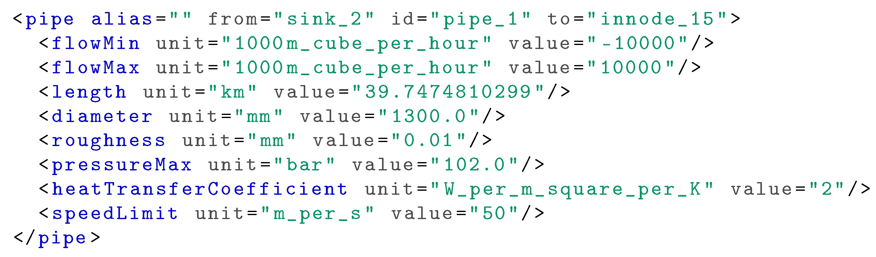
Pipes are specified by the additional parameters length, diameter, and roughness; see Figure 9. These are used to compute the friction factor in the pressure loss equation. The pressureMax element specifies the maximum pressure that the material of the pipe can withstand. It is typically used to also bound the pressure on the incident nodes. The heatTransferCoefficient element specifies the heat transfer coefficient of the material of the pipe’s wall, and, finally, the speedLimit element specifies the maximum velocity of the gas in the pipe. The latter parameter is optional. A typical value is 50 .
Short pipes can be interpreted as pipes with zero length and thus do not induce any pressure loss. In particular, this means that the tail and head node of a short pipe have the same location. A shortPipe has no further attributes; see Figure 10 for an example.
A resistor is an artificial network element that serves as a surrogate for elements such as measurement devices or filters. These elements are typically not captured exactly in simulation or optimization models but lead to a pressure loss that should be modeled. Two types of resistors appear in the GasLib instances. One results in a constant pressure loss (in the direction of the flow), which is specified by the element pressureLoss. The other type induces a pressure loss that continuously depends on the flow rate through the resistor as specified by the tags dragFactor and diameter. An example for both types of resistors is given in Figure 11.
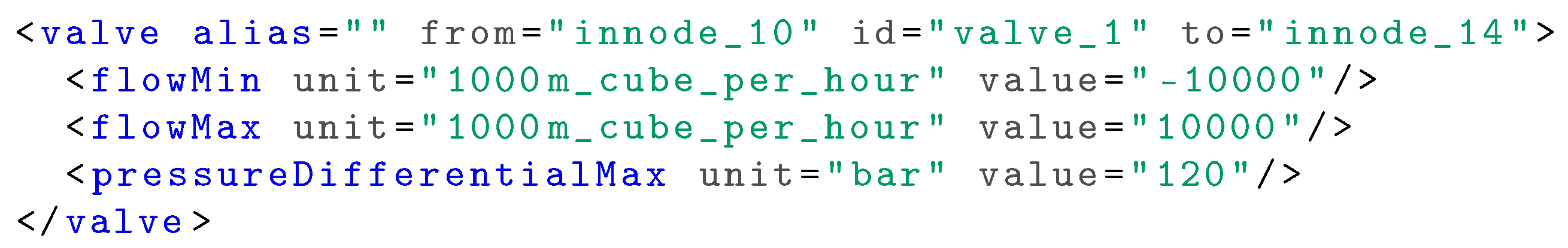
The elements specified by the type valve can be open or closed. In the open state, the pressures at the end nodes attain the same value, while in the closed state, the flow rate is zero. They only have one specific parameter pressureDifferentialMax that restricts the difference of pressures between the from and to node when the valve is closed; see Figure 12 for an example.
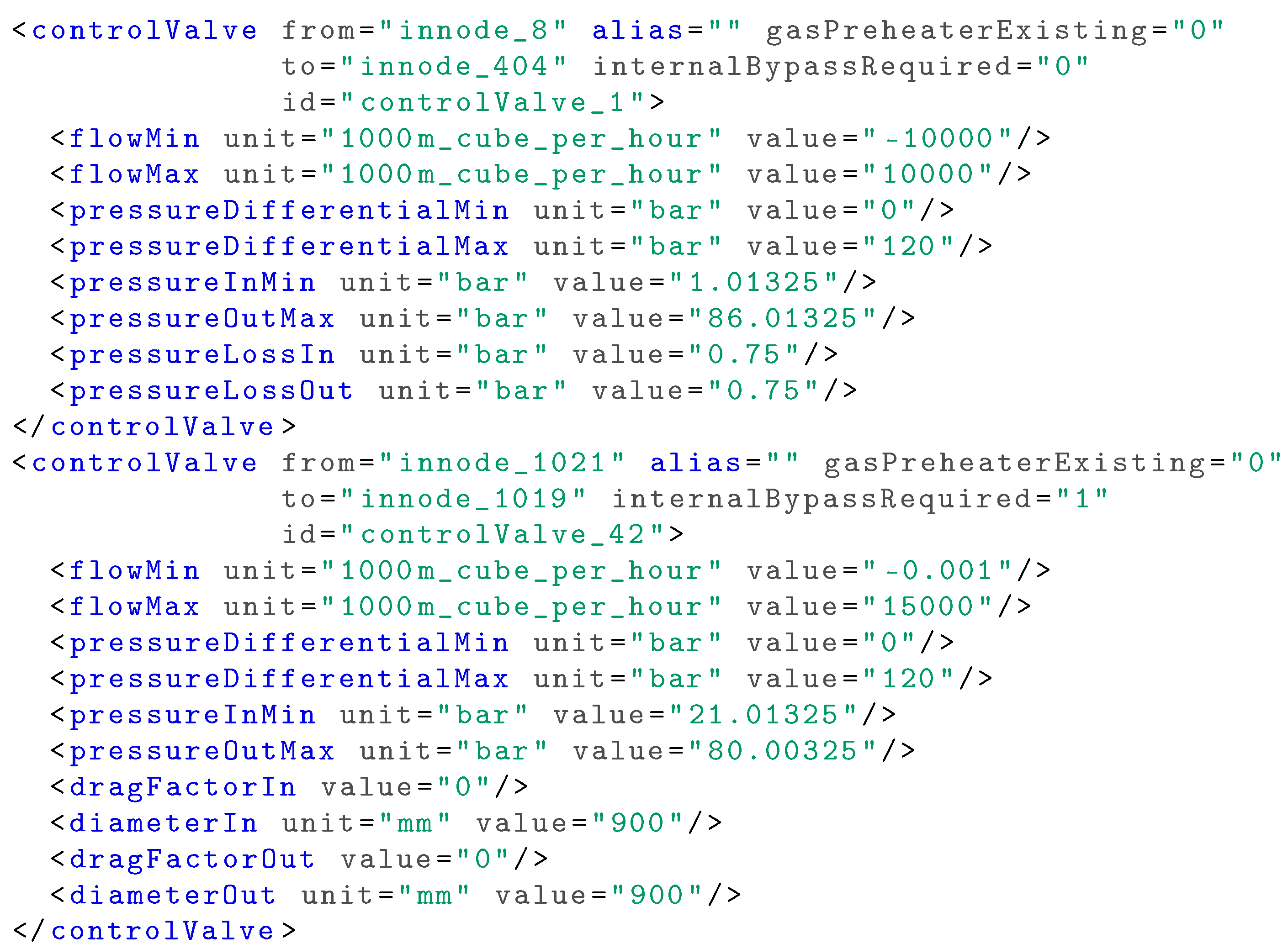
There are two variants of controlValve elements, as shown in Figure 13. These elements can be set to three states: active, bypass mode, and closed. In the active state, gas pressure can be reduced (in the direction of the orientation of the arc), and the parameters pressureDifferentialMin and pressureDifferentialMax define the range of possible pressure reductions. The bypass and closed states are equivalent to the corresponding states of valves. This means that a control valve in bypass mode may have nonzero flow and does not influence the pressures, whereas a closed control valve blocks the gas flow. The attribute internalBypassRequired specifies whether the bypass state needs to be modeled (if 1) or whether a bypass valve is already given in the network topology. The controlValve elements have resistors at their inlet and outlet, which are described with the same data as stand-alone resistors. The resistors only have to be considered if the controlValve is active. Otherwise, they do not have any impact on the gas flow. Finally, the attribute gasPreheaterExisting specifies if a gas preheater is present at the control valve station.
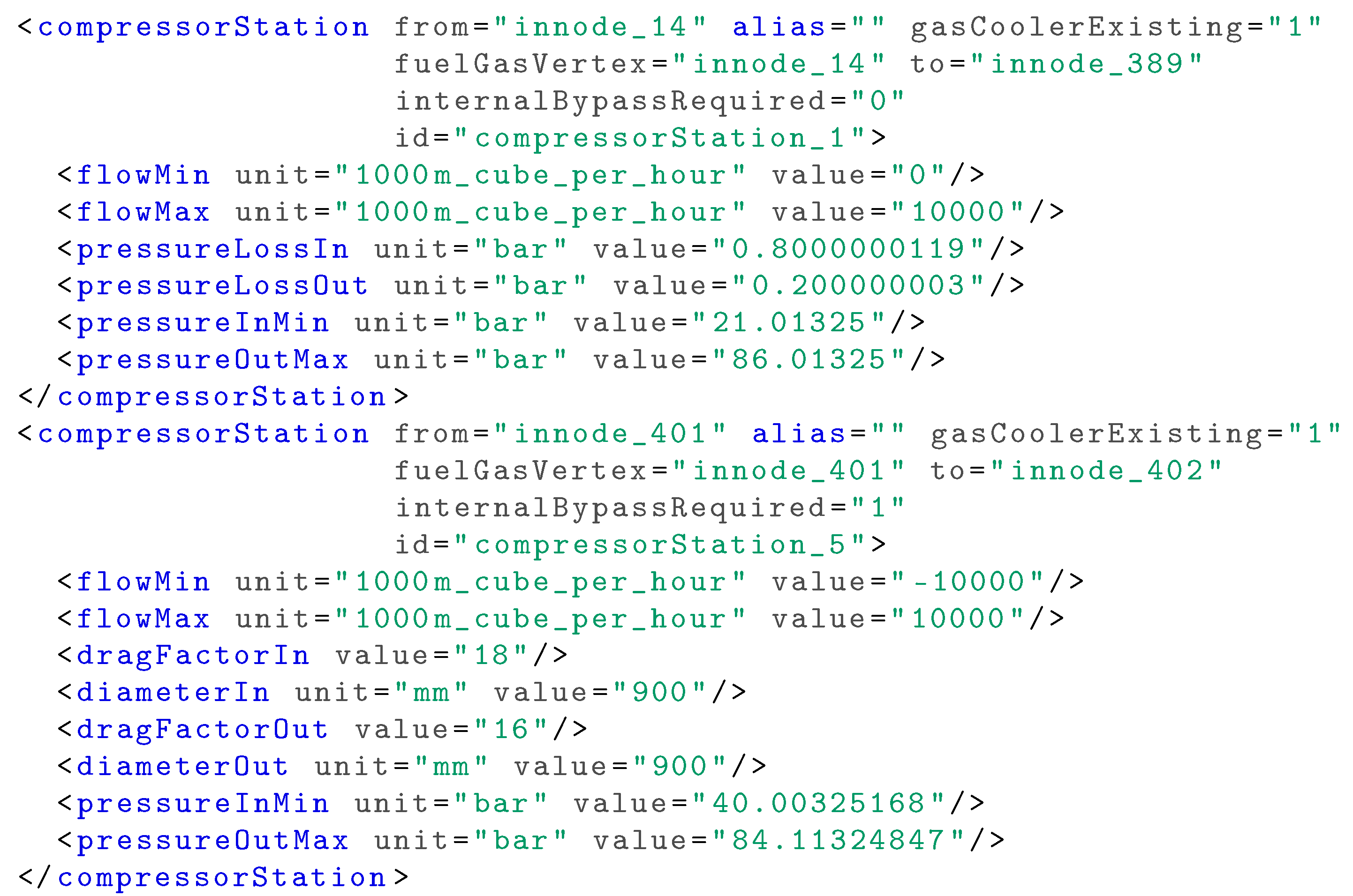
Compressor stations are also given in two variants depending on the type of the included resistors; see Figure 14 for the examples. The attribute fuelGasVertex specifies the node from which the fuel gas is taken, and the attribute gasCoolerExisting specifies whether a gas cooler is installed at the station or not. We note that the description of the compressorStation in the net file is not complete. The hosted machines are the most complicated elements of the considered networks, which is the reason why they are described in a separate cs file; see Section 2.2.2.
2.2.2. The cs File
The full specification of the compressor stations listed in a net file is given in a cs file. These files describe all compressor machines and their drives. In addition, a list of configurations is given that defines the set of possible interconnections of the machines in the station.
Most of the machines that are hosted in compressor stations can be described by characteristic diagrams that are achieved by least-squares fits of (bi-)quadratic functions to a given set of measurements. In cs files, both a parameterization of the fitted functions as well as the measurements are given.
In order to describe the XML format below, we briefly state the ansatz functions for the fits: For quadratic functions , we have , where and . For biquadratic functions , we have with , and . More details about the technical and physical background as well as on the mathematical modeling can be found in [4] or [22].
Every compressor station hosts a certain number of compressor machines. GasLib distinguishes two types of compressor machines: turbo and piston compressors. Turbo compressors are described by characteristic diagrams in the -space, where Q is the volumetric flow rate through the compressor, is the adiabatic change in specific enthalpy, n is the speed of the machine, and denotes the adiabatic efficiency of the compression process. The meaning of this quadruple can be summarized as follows: the turbo compressor is able to compress a volumetric flow rate Q with an adiabatic change in specific enthalpy using a compressor speed of n and yielding an efficiency of ; see Figure 15.
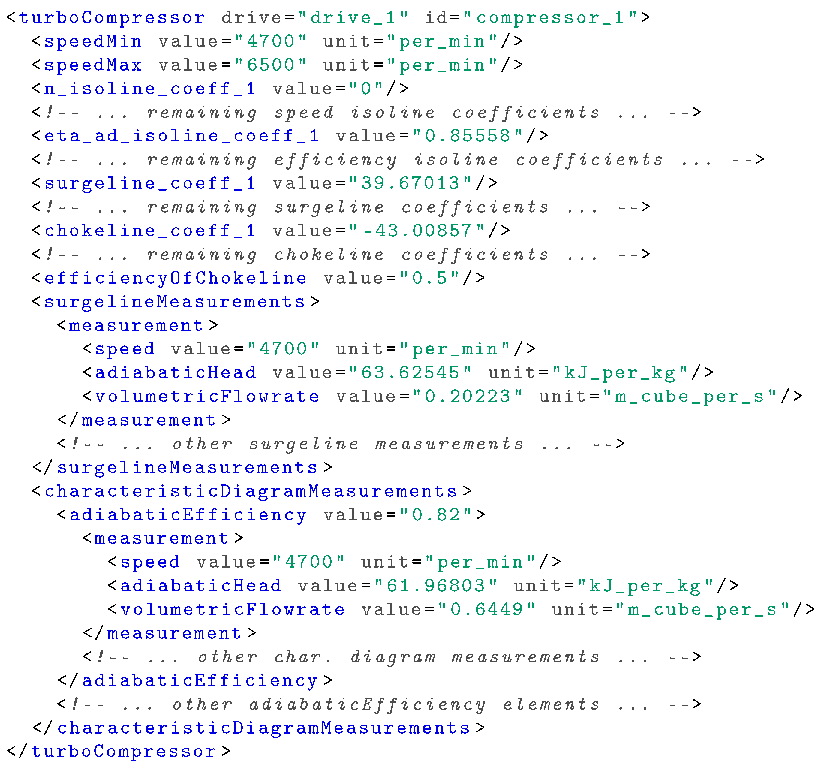
The quadruples given for a specific machine are obtained by measurements that are given in the characteristicDiagramMeasurements element of the turbo compressor; see Figure 16. The biquadratic fits are given in the cs file by the coefficients n_isoline_coeff_1,…, n_isoline_coeff_9 for the biquadratic isolines of the speed of the machine (solid lines in Figure 15), and the coefficients eta_ad_isoline_coeff_1,…, eta_ad_isoline_coeff_9 for the biquadratic isolines of adiabatic efficiency (dashed lines in Figure 15). The upper and lower bounds of the characteristic diagram are given by the isolines of speed together with the minimum speed speedMin as well as the maximum speed speedMax, respectively. The left and right border, that is, the surgeline and the chokeline of the machine, are given separately as quadratic functions (of the volumetric flow rate Q) with coefficients surgeline_coeff_1,…, surgeline_coeff_3 and chokeline_coeff_1,…, chokeline_coeff_3, respectively. The chokeline efficiency is given explicitly in the element efficiencyOfChokeline, whereas the surgeline is specified by its measurements contained in the element surgelineMeasurements. These measurements are given by triples of speed, adiabaticHead, and volumetricFlowrate. All other measurements of the characteristic diagram are given in the element characteristicDiagramMeasurements, which lists sets of such triples for every measured adiabaticEfficiency.
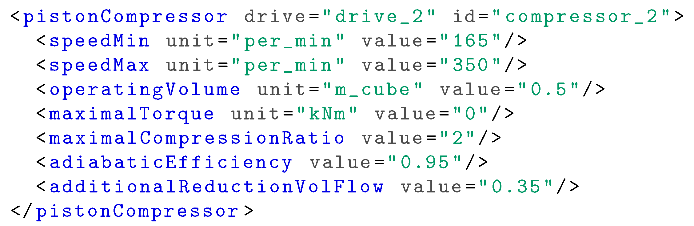
The data format for piston compressors is easier; see Figure 17. Piston compressors are mainly characterized by the volume (operatingVolume), which fits into their compression cylinder, and by the minimal speed (speedMin) and maximal speed (speedMax) they can be operated in. Additionally, the maximal torque (maximalTorque) of the piston compressor’s crankshaft, the maximal compression ratio (maximalCompressionRatio), and the adiabatic efficiency (adiabaticEfficiency) of the compression process are specified. The volumetric flow rate through the piston compressor depends on the rotational speed of the crankshaft. Operating the piston compressor at its minimal speed therefore gives a lower bound on the volumetric flow rate. However, for some piston compressors, decreasing the volumetric flow by technical means to a level that is lower than the aforementioned bound is required. If this is the case, the reducing factor is given by the element additionalReductionVolFlow.
Every compressor is mounted on a drive that delivers the compressor with the required power. Drives are described by their specific energy consumption rate that is given as a quadratic fit with coefficients energy_rate_fun_coeff_1,…, energy_rate_fun_coeff_3 and the maximum power function. This depends on the specific drive type if the latter is modeled by a quadratic function of the compressor’s speed (with coefficients power_fun_coeff_1,…, power_fun_coeff_3) or by a biquadratic function of the compressor’s speed and the ambient temperature at the station (with coefficients power_fun_coeff_1,…, power_fun_coeff_9). For exemplary XML specifications, see Figure 18. For further details on modeling drives, we refer the reader to [4,21,29].
Finally, the cs file contains a list of configurations for every compressor station; see Figure 19. A configuration is a serial arrangement of parallel combinations of compressor machines, and the element configurations lists all possible configurations for the corresponding station.
2.2.3. The cdf File
The cdf file optionally complements the net file by describing additional restrictions for the switching of certain sets of controllable elements (valve, controlValve, and compressorStation).
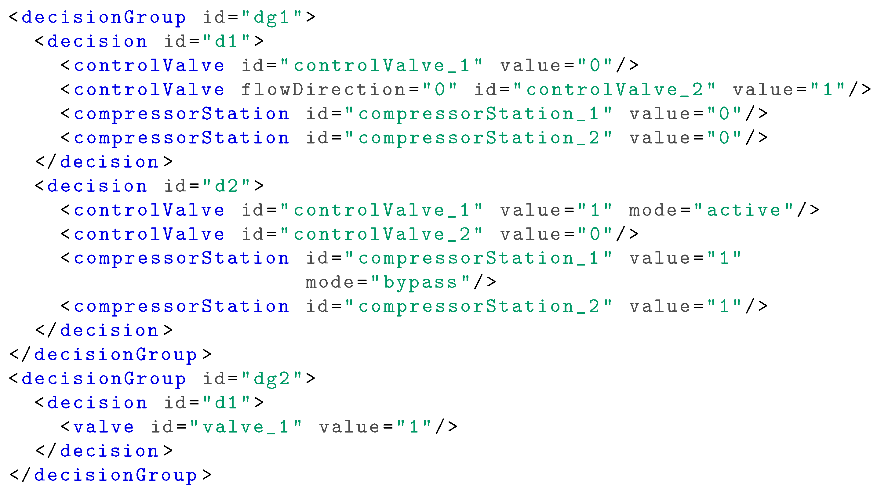
Besides compressor machines, there are many other elements in real-world compressor or control valve stations that are used to increase the flexibility of the network operator, for example, for routing the gas near the stations in different directions. The interplay of these sets of network elements is described in the cdf file. We call the grouped sets of controllable elements “subnetworks”, and the restrictions of their interplay are called “combined decisions”. A subnetwork is modeled as a decisionGroup in the data format, and the corresponding set of possible switching decisions for the elements of the subnetwork are modeled as a list of the element decision; see Figure 20 for examples. One decision must be chosen, with implications for the arcs in the decisionGroup: For a value of 0, the corresponding network element is closed. For a value of 1, it is open and maybe active or in bypass mode. Optionally, for each arc, a flowDirection (0 or 1 for backward or forward flow) and a mode (active or bypass) may be given. If a decisionGroup contains only a single decision, this effectively fixes the switching decisions for the affected arcs. This is used, for example, in the GasLib-4197 instance to fix certain valve elements that are not remote-controlled.
2.2.4. The scn File
The scn file specifies a demand and supply scenario for a network. Thus, a gas transport instance is only given completely by the combination of a network (with a net, a cs, and an optional cdf file) together with an scn file. GasLib contains a single scenario file for the four small- to medium-scale networks GasLib-11, GasLib-24, GasLib-40, and GasLib-135 and many different scn files for the real-world networks GasLib-134, GasLib-582, and GasLib-4197.
The supplied and discharged amounts of gas at entries and exits can be specified in mass flow q (), normal volumetric flow (), or power P (). The power can be computed from the mass flow q and the calorific value via . The mass flow is computed from the normal volumetric flow and the density under normal conditions via . Conservation of mass at the nodes of the network is typically stated in mass flow q. However, it can also be expressed in the normal volumetric flow if a constant density under normal conditions is assumed throughout the network. All flow bounds in the net and scn files of GasLib are expressed in normal volumetric flow, as this is the standard unit in gas transport.
In stationary models of gas flow, the supplied and discharged values must be in balance, that is, the sum of the supplies at the source nodes equals the sum of the discharged flows at the sink nodes. The flow values in all scn files of GasLib are fixed to values that satisfy this balance constraint. Thus, all provided scn files define nominations, as described in the introduction.
For every node in the scn file, a type is specified: entry or exit. Typically, nodes that are a source (sink) in the net file should be an entry (exit) in the scn file. Otherwise, the sign of the corresponding flow value has to be changed.
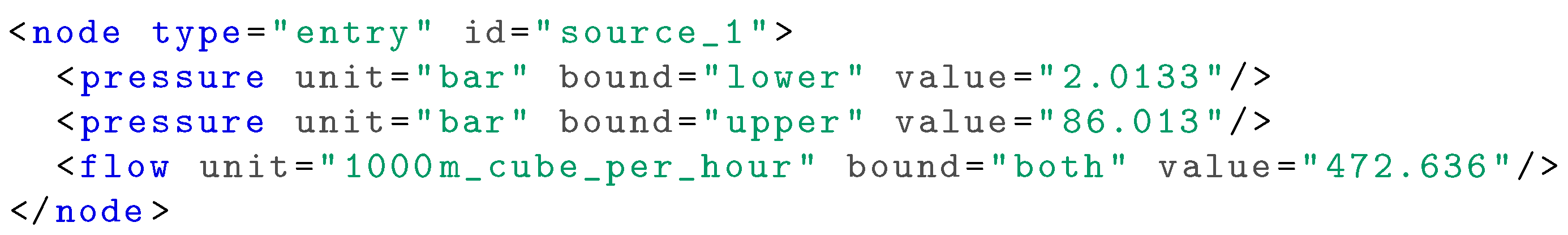
Finally, pressure bounds may be specified for the nodes. These bounds should be intersected with the bounds from the net file, that is, the tightest bound holds. Typically, lower pressure bounds are given for exits, and upper pressure bounds are given for entries. Optionally, contractPressure bounds may be specified for further restricting the allowed pressure values.
See Figure 21 for an exemplary specification of pressure bounds and a fixation of the flow amount in an scn file.
3. Outlook
The next steps in the further development of GasLib are to add more and even larger instances. Moreover, we also plan to provide transient data in the near future. In any case, GasLib will only be successful if it is used. Moreover, we are always grateful for constructive remarks and, of course, for providing new data.
Acknowledgments
This work has partially been supported by the German Federal Ministry of Economics and Technology owing to a decision of the German Bundestag. We are very grateful to our former industry partner Open Grid Europe GmbH for providing us with the real-world network and nomination data, as well as for numerous discussions on that topic. Finally, we thank all collaborators of the ForNe project, that is, all associated researchers from Zuse Institute Berlin, Friedrich-Alexander-Universität Erlangen-Nürnberg, Leibniz Universität Hannover, University of Duisburg-Essen, Humboldt University zu Berlin, TU Darmstadt, and WIAS Institute in Berlin. We further acknowledge funding through the DFG SFB/Transregio 154, subprojects A01, A05, A07, B06, B07, B08, Z01, Z02.
Author Contributions
All authors collected, analyzed, and prepared the data that are part of GasLib. All authors jointly wrote the paper.
Conflicts of Interest
The authors declare no conflict of interest.
References
- Evaluating Gas Network Capacities; Koch, T.; Hiller, B.; Pfetsch, M.E.; Schewe, L. (Eds.) SIAM: Philadelphia, PA, USA, 2015. [Google Scholar]
- Pfetsch, M.E.; Fügenschuh, A.; Geißler, B.; Geißler, N.; Gollmer, R.; Hiller, B.; Humpola, J.; Koch, T.; Lehmann, T.; Martin, A.; et al. Validation of nominations in gas network optimization: Models, methods, and solutions. Optim. Methods Softw. 2015, 30, 15–53. [Google Scholar] [CrossRef]
- Ríos-Mercado, R.Z.; Borraz-Sánchez, C. Optimization Problems in Natural Gas Transportation Systems: A State-of-the-Art Review. Appl. Energy 2015, 147, 536–555. [Google Scholar] [CrossRef]
- Fügenschuh, A.; Geißler, B.; Gollmer, R.; Morsi, A.; Pfetsch, M.E.; Rövekamp, J.; Schmidt, M.; Spreckelsen, K.; Steinbach, M.C. Physical and technical fundamentals of gas networks. In Evaluating Gas Network Capacities; Koch, T., Hiller, B., Pfetsch, M.E., Schewe, L., Eds.; SIAM: Philadelphia, PA, USA, 2015; Chapter 2; pp. 17–43. [Google Scholar]
- De Wolf, D.; Smeers, Y. The Gas Transmission Problem Solved by an Extension of the Simplex Algorithm. Manag. Sci. 2000, 46, 1454–1465. [Google Scholar] [CrossRef]
- General Algebraic Modeling System. Available online: http://gams.com (accessed on 1 November 2017).
- Geißler, B.; Martin, A.; Morsi, A.; Schewe, L. The MILP-relaxation approach. In Evaluating Gas Network Capacities; Koch, T., Hiller, B., Pfetsch, M.E., Schewe, L., Eds.; SIAM: Philadelphia, PA, USA, 2015; Chapter 6; pp. 103–122. [Google Scholar]
- Ehrhardt, K.; Steinbach, M.C. Nonlinear Optimization in Gas Networks. In Modeling, Simulation and Optimization of Complex Processes; Bock, H.G., Kostina, E., Phu, H.X., Rannacher, R., Eds.; Springer: Berlin, Germany, 2005; pp. 139–148. [Google Scholar]
- Gugat, M.; Leugering, G.; Martin, A.; Schmidt, M.; Sirvent, M.; Wintergerst, D. MIP-Based Instantaneous Control of Mixed-Integer PDE-Constrained Gas Transport Problems. Comput. Optim. Appl. 2017. [Google Scholar] [CrossRef]
- Hante, F.M.; Schmidt, M. Complementarity-Based Nonlinear Programming Techniques for Optimal Mixing in Gas Networks; Technical Report; FAU Erlangen-Nürnberg: Erlangen, Germany, 2017; Available online: http://www.optimization-online.org/DB_HTML/2017/09/6198.html (accessed on 29 November 2017).
- Humpola, J. Gas Network Optimization by MINLP. Ph.D. Thesis, Technische Universität Berlin, Berlin, Germany, 2014. [Google Scholar]
- Borraz-Sánchez, C.; Bent, R.; Backhaus, S.; Hijazi, H.; van Hentenryck, P. Convex Relaxations for Gas Expansion Planning. INFORMS J. Comput. 2016, 28, 645–656. [Google Scholar] [CrossRef]
- Mak, T.W.K.; Van Hentenryck, P.; Zlotnik, A.; Hijazi, H.; Bent, R. Efficient Dynamic Compressor Optimization in Natural Gas Transmission Systems; Technical Report; 2015; Available online: https://arxiv.org/abs/1511.07562 (accessed on 29 November 2017).
- Groß, M.; Pfetsch, M.E.; Schewe, L.; Schmidt, M.; Skutella, M. Algorithmic Results for Potential-Based Flows: Easy and Hard Cases; Technical Report; 2017; Available online: http://www.optimization-online.org/DB_HTML/2017/08/6185.html (accessed on 29 November 2017).
- Habeck, O.; Pfetsch, M.E.; Ulbrich, S. Global Optimization of ODE Constrained Network Problems on the Example of Stationary Gas Transport. Available online: http://www.optimization-online.org/DB_HTML/2017/10/6288.html (accessed on 29 November 2017).
- DESFA. Available online: http://www.desfa.gr (accessed on 1 November 2017).
- Sirvent, M.; Kanelakis, N.; Geißler, B.; Biskas, P. Linearized model for optimization of coupled electricity and natural gas systems. J. Mod. Power Syst. Clean Energy 2017, 5, 364–374. [Google Scholar] [CrossRef]
- Gugat, M.; Leugering, G.; Martin, A.; Schmidt, M.; Sirvent, M.; Wintergerst, D. Towards Simulation Based Mixed-Integer Optimization with Differential Equations; Technical Report; FAU Erlangen-Nürnberg: Erlangen, Germany, 2016; Available online: http://www.optimization-online.org/DB_HTML/2016/07/5542.html (accessed on 29 November 2017).
- Schmidt, M.; Sirvent, M.; Wollner, W. A Decomposition Method for MINLPs with Lipschitz Continuous Nonlinearities; Technical Report; 2017; Available online: http://www.optimization-online.org/DB_HTML/2017/07/6130.html (accessed on 29 November 2017).
- Hiller, B.; Hayn, C.; Heitsch, H.; Henrion, R.; Leövey, H.; Möller, A.; Römisch, W. Methods for verifying booked capacities. In Evaluating Gas Network Capacities; Koch, T., Hiller, B., Pfetsch, M.E., Schewe, L., Eds.; SIAM: Philadelphia, PA, USA, 2015; Chapter 14; pp. 291–315. [Google Scholar]
- Schmidt, M.; Steinbach, M.C.; Willert, B.M. High detail stationary optimization models for gas networks: Validation and results. Optim. Eng. 2016, 17, 437–472. [Google Scholar] [CrossRef]
- Rose, D.; Schmidt, M.; Steinbach, M.C.; Willert, B.M. Computational optimization of gas compressor stations: MINLP models versus continuous reformulations. Math. Methods Oper. Res. 2016, 83, 409–444. [Google Scholar] [CrossRef]
- Burlacu, R.; Geißler, B.; Schewe, L. Solving Mixed-Integer Nonlinear Programs Using Adaptively Refined Mixed-Integer Linear Programs; Technical Report; FAU Erlangen-Nürnberg: Erlangen, Germany, 2017; Available online: https://opus4.kobv.de/opus4-trr154/frontdoor/index/index/docId/151 (accessed on 29 November 2017).
- Hennig, K.; Schwarz, R. Using Bilevel Optimization to find Severe Transport Situations in Gas Transmission Networks; Technical Report 16-68; Zuse Institute Berlin (ZIB): Berlin, Germany, 2016. [Google Scholar]
- Geißler, B.; Morsi, A.; Schewe, L.; Schmidt, M. Solving power-constrained gas transportation problems using an MIP-based alternating direction method. Comput. Chem. Eng. 2015, 82, 303–317. [Google Scholar] [CrossRef]
- Geißler, B.; Morsi, A.; Schewe, L.; Schmidt, M. Solving Highly Detailed Gas Transport MINLPs: Block Separability and Penalty Alternating Direction Methods. INFORMS J. Comput. 2017. Available online: http://www.optimization-online.org/DB_HTML/2016/06/5523.html (accessed on 30 November 2017).
- Extensible Markup Language (XML). Available online: https://www.w3.org/XML/ (accessed on 16 November 2017).
- W3C XML Schema Definition Language (XSD). Available online: https://www.w3.org/TR/xmlschema11-1/ (accessed on 16 November 2017).
- Schmidt, M.; Steinbach, M.C.; Willert, B.M. The precise NLP model. In Evaluating Gas Network Capacities; Koch, T., Hiller, B., Pfetsch, M.E., Schewe, L., Eds.; SIAM: Philadelphia, PA, USA, 2015; Chapter 10; pp. 181–210. [Google Scholar]
Figure 1.
Schematic plot of the GasLib-11 network.
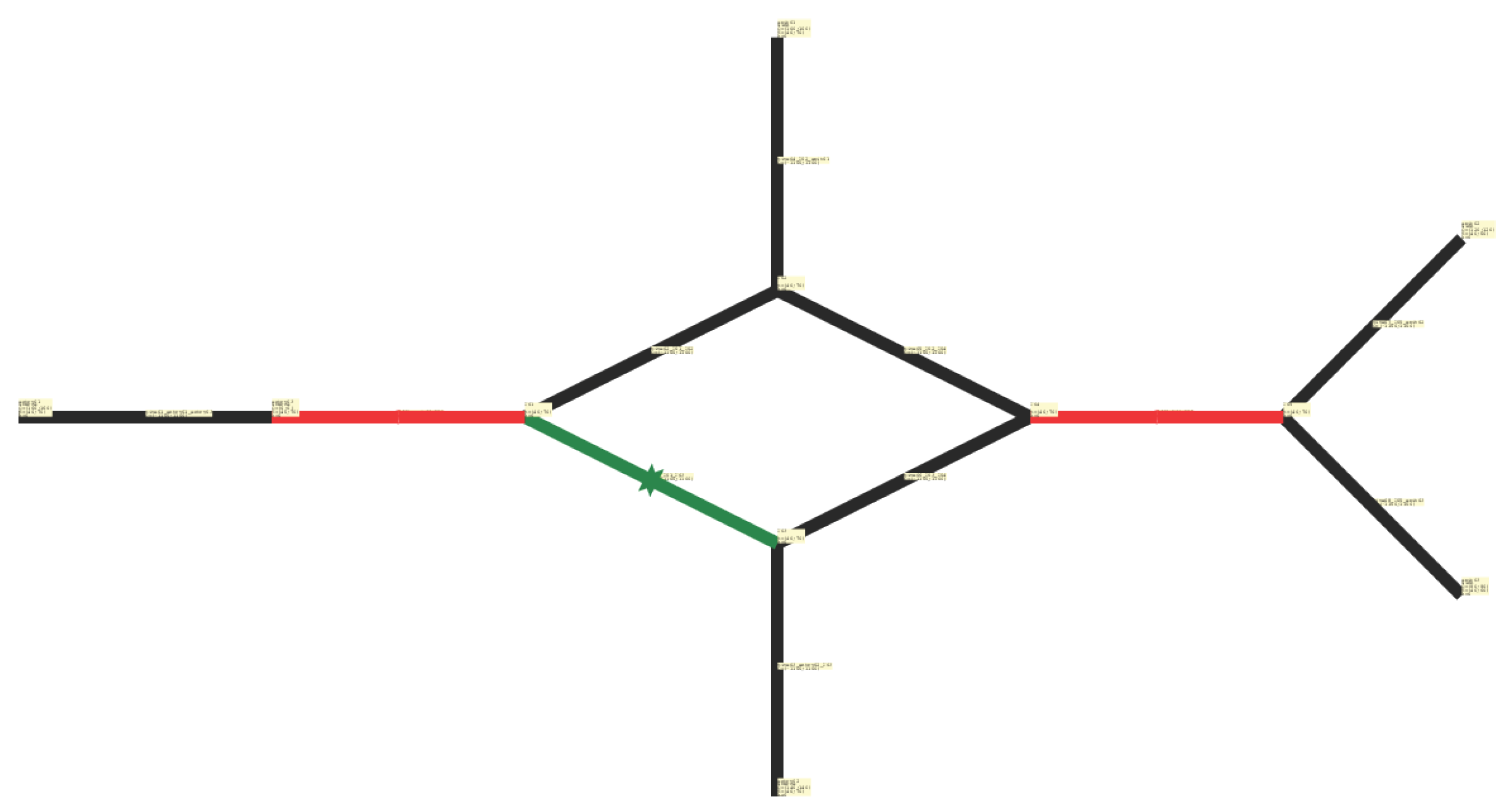
Figure 2.
Schematic plot of the GasLib-24 network.

Figure 3.
Schematic plot of the GasLib-40 network.

Figure 4.
Schematic plot of the GasLib-134 network.
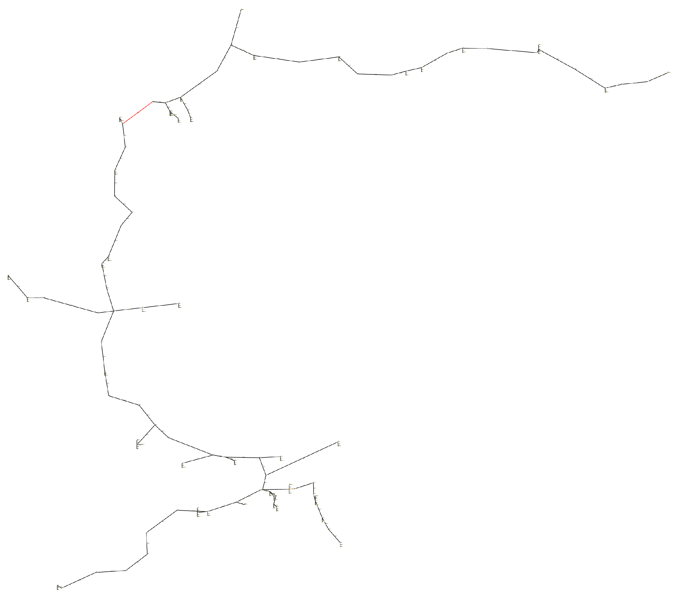
Figure 5.
Schematic plot of the GasLib-135 network.

Figure 6.
Schematic plot of the GasLib-582 network.
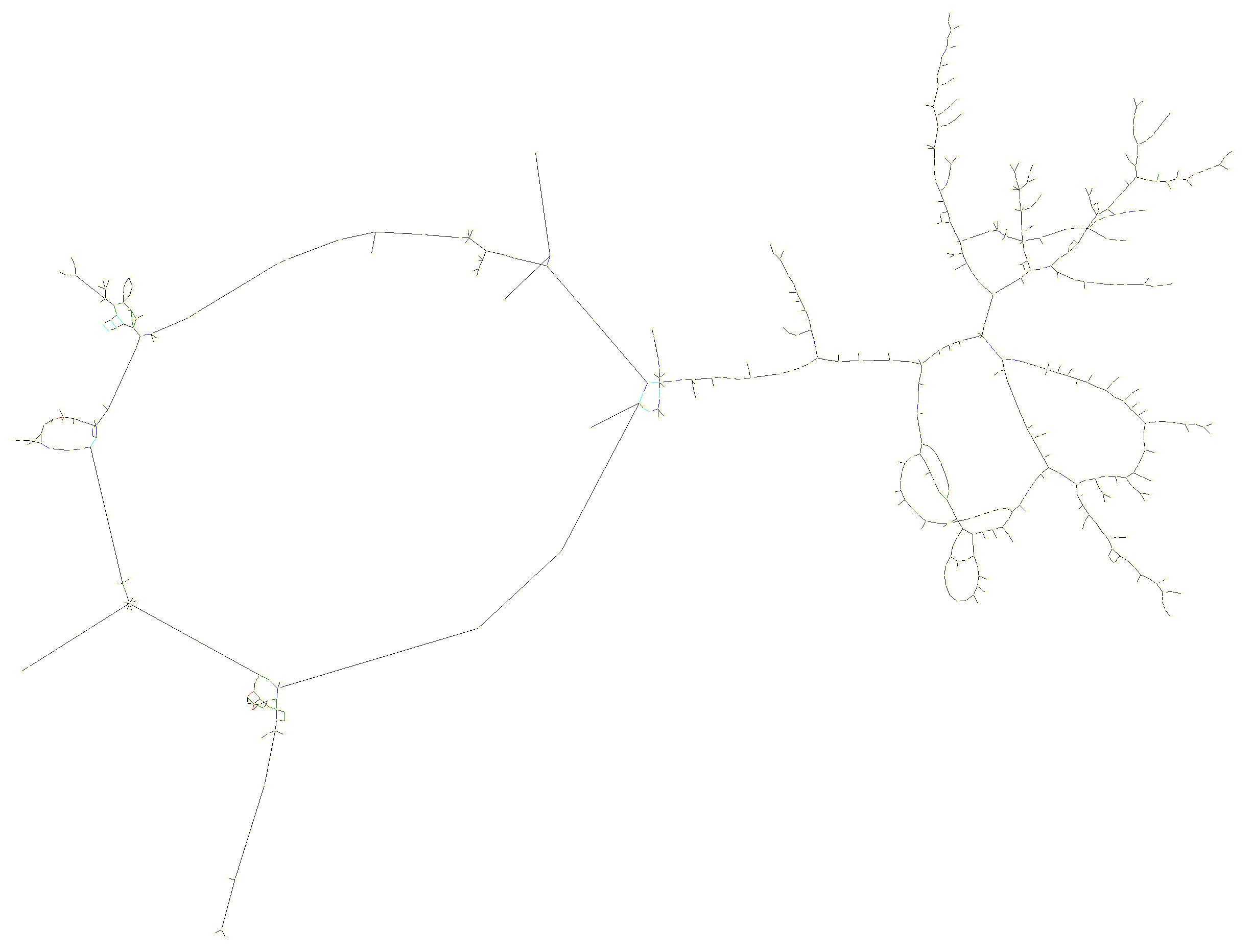
Figure 7.
Schematic plot of the GasLib-4197 network.
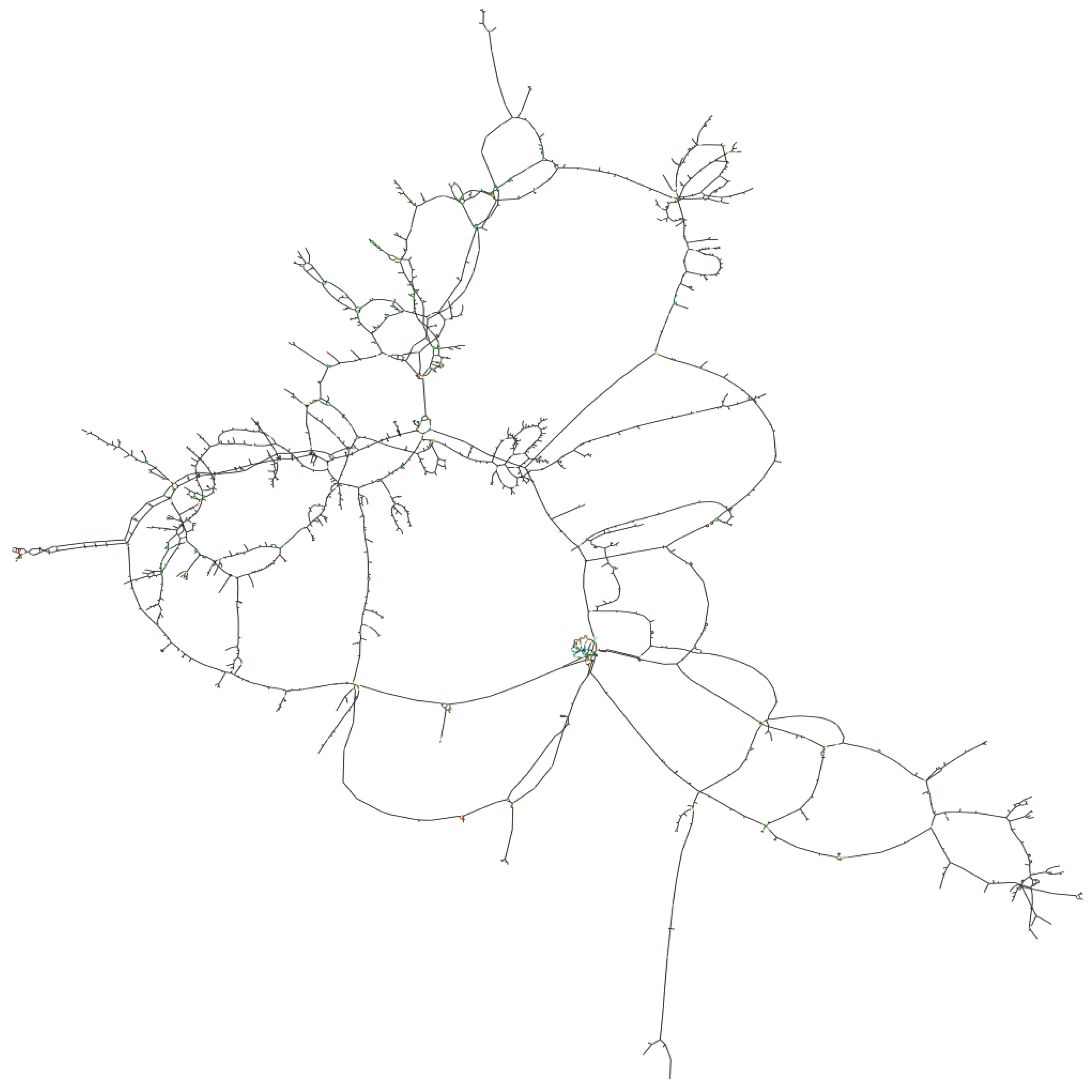
Figure 8.
Examples of source, sink, and innode in the net file.
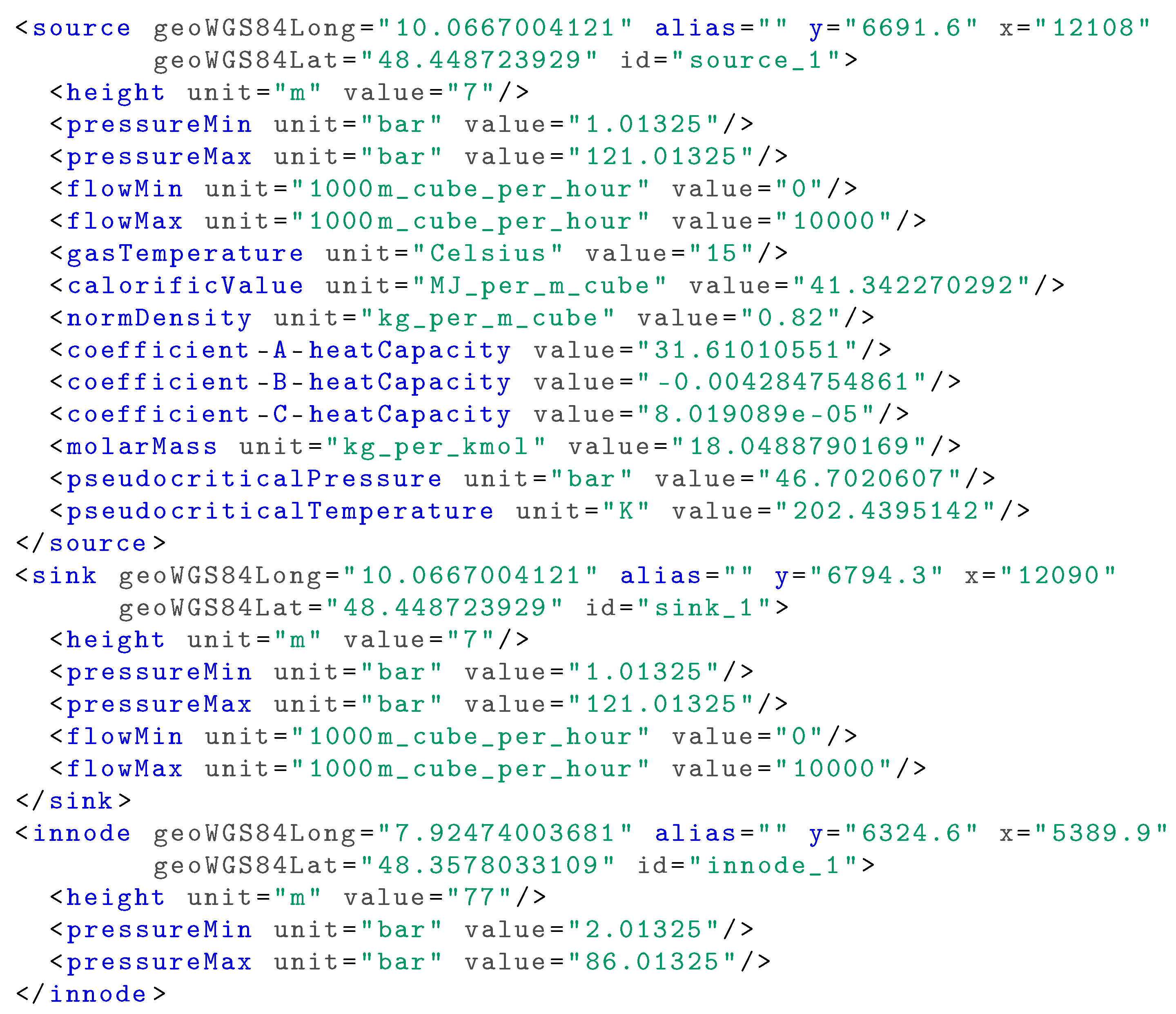
Figure 9.
Example of pipe in the net file.

Figure 10.
Example of shortPipe in the net file.
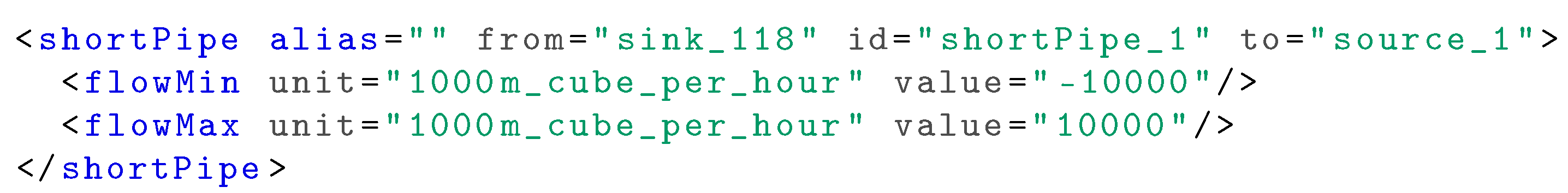
Figure 11.
Example of two resistor types in the net file.
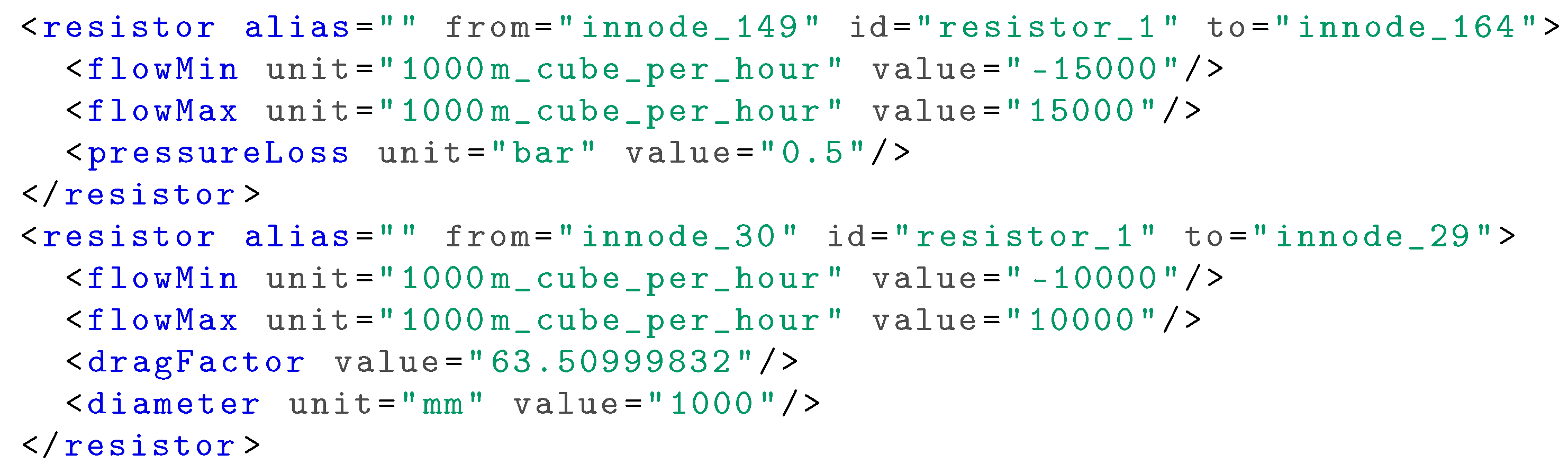
Figure 12.
Example of valve in the net file.

Figure 13.
Example of two types of controlValve in the net file.

Figure 14.
Example of two types of compressorStation in the net file.

Figure 15.
Characteristic diagram of an exemplary turbo compressor.
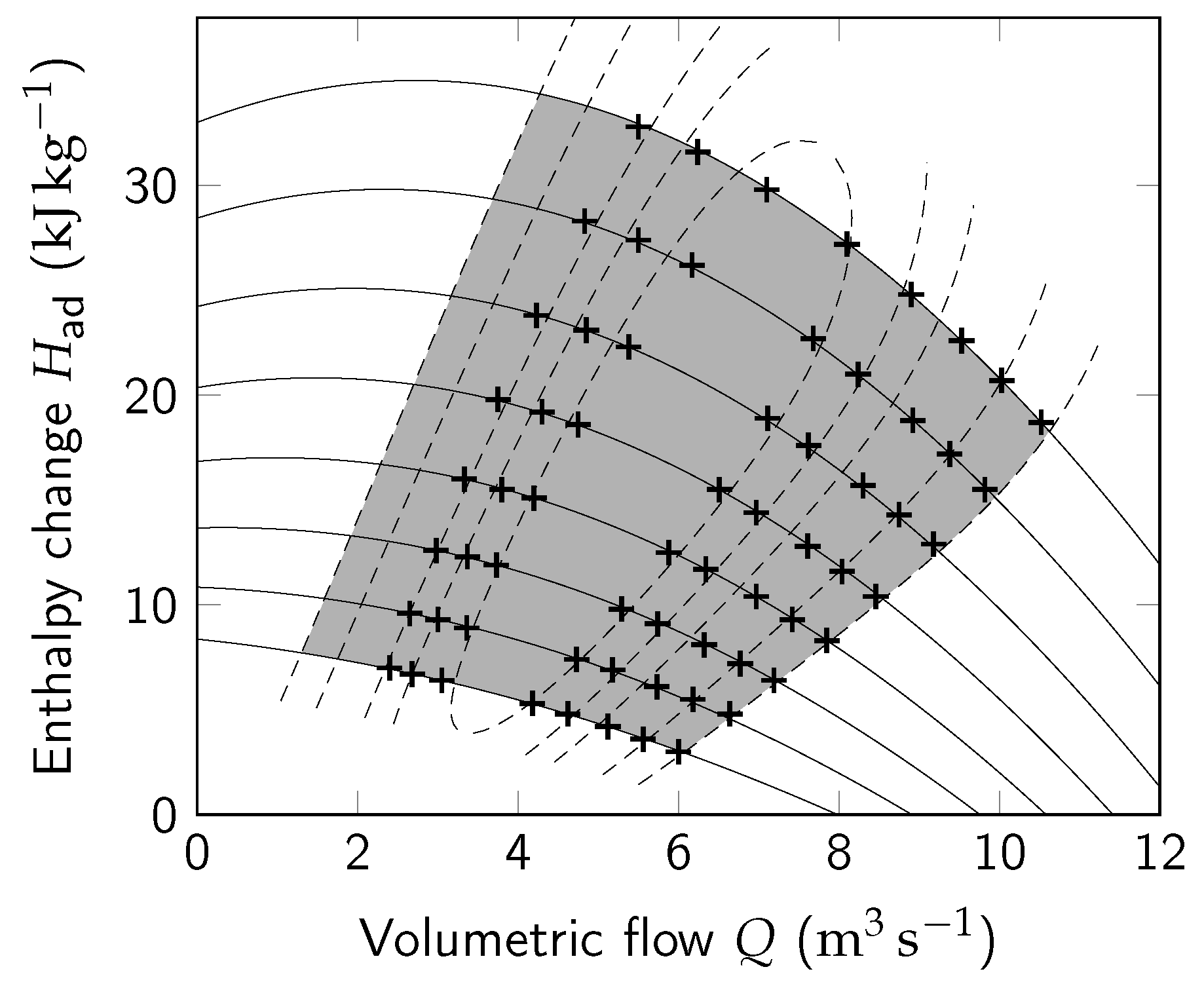
Figure 16.
Exemplary definition of a turbo compressor in a cs file.

Figure 17.
Exemplary specification of a piston compressor in a cs file.

Figure 18.
Example of the specification of a gas turbine and a gas-driven motor in a cs file.
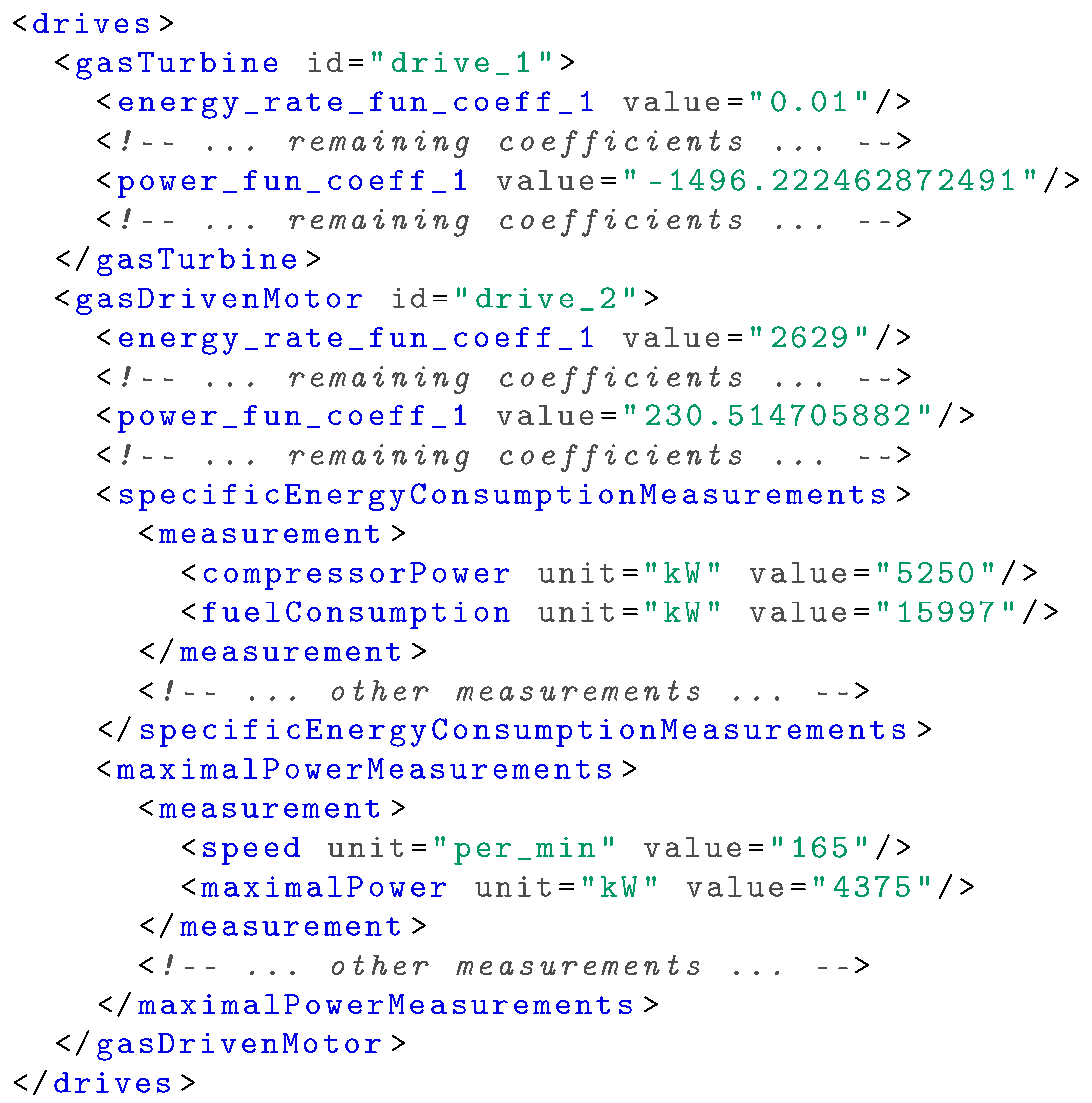
Figure 19.
Example of two configurations in a cs file.
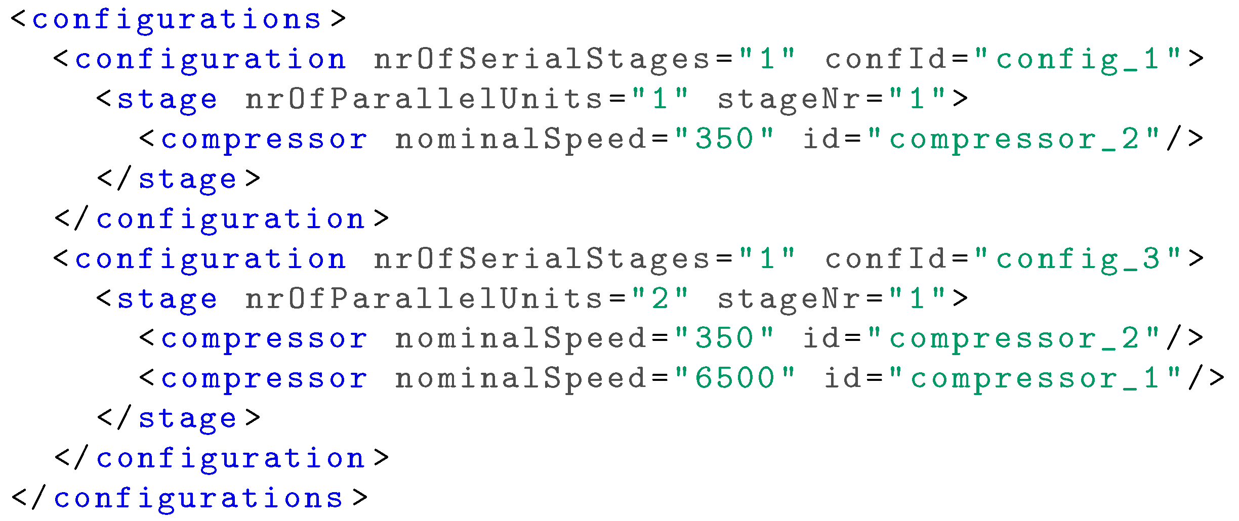
Figure 20.
Two examples for a decisionGroup of a cdf file.

Figure 21.
An exemplary node specification from an scn file.


Table 1.
Exemplary units that are supported by GasLib.
| Physical/Technical Quantity | Units |
|---|---|
| Gas flow | , , 1000 , … |
| Gas temperature | C, , … |
| Length | , , , , … |
© 2017 by the authors. Licensee MDPI, Basel, Switzerland. This article is an open access article distributed under the terms and conditions of the Creative Commons Attribution (CC BY) license (http://creativecommons.org/licenses/by/4.0/).
Share and Cite
MDPI and ACS Style
Schmidt, M.; Aßmann, D.; Burlacu, R.; Humpola, J.; Joormann, I.; Kanelakis, N.; Koch, T.; Oucherif, D.; Pfetsch, M.E.; Schewe, L.; et al. GasLib—A Library of Gas Network Instances. Data 2017, 2, 40. https://doi.org/10.3390/data2040040
AMA Style
Schmidt M, Aßmann D, Burlacu R, Humpola J, Joormann I, Kanelakis N, Koch T, Oucherif D, Pfetsch ME, Schewe L, et al. GasLib—A Library of Gas Network Instances. Data. 2017; 2(4):40. https://doi.org/10.3390/data2040040
Chicago/Turabian StyleSchmidt, Martin, Denis Aßmann, Robert Burlacu, Jesco Humpola, Imke Joormann, Nikolaos Kanelakis, Thorsten Koch, Djamal Oucherif, Marc E. Pfetsch, Lars Schewe, and et al. 2017. "GasLib—A Library of Gas Network Instances" Data 2, no. 4: 40. https://doi.org/10.3390/data2040040