1. Introduction
As the boundaries and population of urban areas expand, beverage distributors may seek to expand capacity in their distribution centers. As a result, they may need to add new locations or increase the utilization of their existing centers. This study identifies new warehouse locations for efficient logistical activities by quantifying transportation costs associated with increasing demand. Potential alternative locations could be located in the current urban areas or in new industrial parks designated by cities. The cities of Fargo, ND, Moorhead, MN, and West Fargo, ND, are selected as potential candidates for a distribution center in this case study. Each city has its own zoning plans, which designate commercial, industrial, and residential boundaries, and restrict development through related regulations. A potential warehouse would be located in areas zoned for commercial and industrial use.
In this case study, the customers of the distributor are dispersed in Eastern North Dakota and Western Minnesota. More than 300 stores, including retailers, restaurants, and bars, are customers of the distributors. Most of these major customers are located in towns with larger populations. In small towns, the restaurants, gas stations, and bars are customers that sell the beverages to consumers.
Distributors’ service routes were designed to fulfill orders from stores, bars, and restaurants. The sequence of the routes vary with the seasons. A variety of routes is used in each season to meet changes in demand. Vehicles serving the routes are constrained by time windows during which they must deliver the orders originating from customers. The vehicles are limited by the load capacity as designed by packaging sizes.
This case study is a location-route problem (LRP) with capacity-limited routes and uncapacitated depots. The objective of the vehicle routings is to minimize the total transportation costs of vehicles and routes [
1], which are subject to the following constraints: (a) only one vehicle serves a customer and a route, (b) all vehicles start at a depot and return to the depot, (c) the capacity of a vehicle should not be exceeded. The integration of facility location problem (FLP) and vehicle routing problem (VRP) is applicable to distribution systems in a beverage industry delivering orders to retail shops and restaurants [
2].
This paper investigates the decomposition method to solve both a location and a routing problem in a practical stage of application. By decomposing an initial combined location-routing problem (LRP) into a vehicle routing problem and location problem and solving them separately, the LRP provides strategic decision for identifying depot location through continuous network space by considering traversable roads links. Geographic Information Systems solve the first component of vehicle routing problem, and then the location was determined by a weighting and ranking method, based on the total transportation costs and mileage. Beverage distributors can use this study as they consider new locations and extra depots to support strategic logistics planning to deal with mid-term and long-term growth of demand in the beverage markets. This study provides a case study of how to apply advanced operations research to real application. It is a way of bringing state-of-the-art spatial technology, such as Geographic Information Systems (GIS), to state-of-practice. Consequently, the decision-making process can be visualized to recognize alternatives in order for logistics planning.
The contribution of this paper is to demonstrate how to integrate the separate vehicle routing problem and facility location problems to choose a preferred location using available tools on hand. Thus, practitioners can adopt the research framework proposed in this paper to support the growing needs of selecting an appropriate location of a depot for beverage business.
2. Literature Review
The location selection is a strategic decision about the facility location of a depot to support increasing customer demand while considering zoning plans in urban areas [
3]. Location selection is strategic decision involving long-term planning and capital investment. While the vehicle routing problem is tactical and to be addressed in consideration of dynamic demand and operational constraints [
4], a vehicle route connecting customers and determining frequency of visiting is strategic to keep strong relationship with the customers. Location problems and vehicle routing problems must be combined to identify potential locations for distribution centers. Extensive studies on location problems and vehicle routing problems are found from broad areas. Locations problems and routing problems are interrelated when it comes to the location-routing problem (LRP).
Nagy and Salhi [
4] review the research about the LRP to address the issues, models, and methods. The paper defined LRP as an integrated solution approach, which considers a hierarchical viewpoint to deal with the strategic decisions of location and routes simultaneously. Thus, the facility problem can be solved as a master problem and the vehicle routing problem as a sub-problem, a so-called two-phase approach. Levy and Bodin [
5] introduced the arc-oriented LRP algorithm using Euler cycles to create a service network (SN) from the travel network. From the service network (SN), the partition network was generated by including some dummy counterpart arcs. The dummy counterpart arcs were connected out of a depot. The study enumerated all potential depots by restricting the maximum number of depots as three in the region showing good performance results. The service network should be connected to run the algorithm in the given network. More recent research are can be found from Prodhon and Print [
6].
In general, LRP attempts to minimize the total cost by selecting potential facilities and constructing delivery routes connecting the selected facilities and demand locations at the same time [
7]. This study is a special case of the LRP problem since a distributor is assumed to build a facility at the optimal location, which will minimize the total vehicle (route) operating costs. Thus, the total demand of customers will be allocated to one depot at a time from a set of potential locations. Each route begins and ends at the same depot, and each customer is served by one vehicle per trip [
6]. The total cost generated by LRP includes three terms: facility cost to open at a depot, the fixed costs of vehicles used, and the route maintenance costs [
6].
This study focuses on the vehicle routing problem to provide the vehicle operating costs since the facility costs is assumed to be homogeneous and the fixed costs of vehicles and routing costs will be combined into vehicle (route) operating costs. A similar concept is found from Tuzun and Burke [
2]. They introduced a two-phase tabu search approach by addressing the facility location problem and the vehicle routing problem simultaneously. The model adopted a demand constraint along a route. They proposed three steps to solve the LRP issue. First, the model initialized by opening a location randomly. Then, the model added a swap from one facility to other candidates. Based on the improved random locations, the VRP finds the best routes of the newly selected locations to compare to the routes from the current facility. They found that a two-phase tabu search algorithm performs reasonably well and requires less computational time. Other works related to the location routing problems are found through review papers for theories and methodologies from Min et al. [
8] and for applications and methods from Nagy and Salhi [
4].
Similarly, Prins
et al. [
9] used the two-phase meta-heuristic method to solve the location-routing problem (LRP): the location phase was solved by a location-facility problem and the routing phase was paired and sequenced by the granular tabu search (GTS) heuristic. In their model, capacity-limited routes and depots were considered to determine the set of depots to locate, and the routes needed from each of the depots, thereby minimizing the total fixed cost to open a depot, establish routes, and the variable cost to operate the routes. Their proposed model reduced the iterations by about 80% compared to other heuristic and meta-heuristics methods. The authors also noted that the results could be obtained for depots that are not capacity limited. Driver-working-hour constraints and customer relationships, which affect the delivery sequence and frequency, can be added to the model as well [
10].
By anchoring the potential locations, the location-routing problem combined with an FLP and VRP reduces to a VRP [
4]. In other words, the vehicle routing problem becomes a sub-problem of LRP, while LRP considers the facility location problem as the master problem in a hierarchical viewpoint [
4]. Then, the vehicle routing problem estimates trucking costs along a route originating from a depot.
The facility location problem can be classified into a multi-objective problem [
11,
12] and multi-attribute location problem [
12]. When we consider the routes to solve location problems, the routes may provide multi-attributes for decision-making criteria, along with the location’s attributes. The routes may be generated by a Euclidean distance between nodes or actual travel distance and time along the real link shapes with respect to speed and driving distance.
Ghiani and Laporte [
13] expanded a Eulerian path-based location problem. Eulerian path visits every node exactly once in a graph from Levy and Bodin [
5]. In the study, they found a set of depots without side constraints on undirected links. The study indicates that the single-depot case of the Eulerian location problem is a particular case of the unbounded case when the potential depot fixed cost is high. A case study of soft-drink distribution is found in Quebec, Canada [
14]. The study solved the vehicle routing problem in consideration of time window, backhaul, and heterogeneous vehicles. The vehicle routing algorithms were introduced in the Geographic Information Systems as an embedded tool. To utilize Geographic Information Systems (GIS), this study focuses on the vehicle operating costs in consideration of time window and heterogeneous vehicles.
Ioannou
et al. [
15] used the Map-Route tool embedded in Map-Info
® GIS software to generate minimum-cost routes using the inter-city vehicle routing problem with time window (VRPTW) and capacity constraints. The application considered one or more depots for picking up orders in order to serve multiple customers en route. The model provided alternative scenarios to answer the potentially significant cost implications. Their solution framework used Euclidean distance and sub-networks to establish routes, therefore, displaying the final outputs in the GIS map for visualization.
Multi-depot vehicle routing problems are found in Laporte
et al. [
1]. Vehicle routing problems are reviewed in detail for local search algorithms by Bräysy and Gendreau [
16] and for meta-heuristics by Bräysy and Gendreau [
17]. Genrdon and Semet [
18] suggested that a path-based location-distribution problem performs better than an arc-based model. A path is generated by a set of arcs, and several paths can be alternatives to select for distribution. In other words, once a path is selected, the path can be used frequently without updating the path as a static model does. The route is strongly interrelated with location model [
11].
GIS, as a spatial decision support tool for solving vehicle routing problems, has been popular since the 1990s and as information technology advances [
19,
20]. Applications can be found for solid waste collection systems [
21,
22], school bus routing [
23], home-health-care nurses [
24], groceries, electronics, bakeries, and cold drinks [
25].
In summary, the vehicle routing problem and location facility problems are well developed. However, implementing integrated method in GIS is critical in a decision-making process because it provides visual information and a practical approach to the practitioners and logistics planners, which are ready to apply. The objective of this case study is (a) to provide solutions to the strategic facility location problem by integrating vehicle routing for intra-city networks considering time window, hours-of-service, capacity, and clustering constraints; (b) to provide an interactive decision making framework using a GIS platform; and (c) to demonstrate the spatial analysis to support strategic decisions for location and operational logistics practices.
3. Model Development
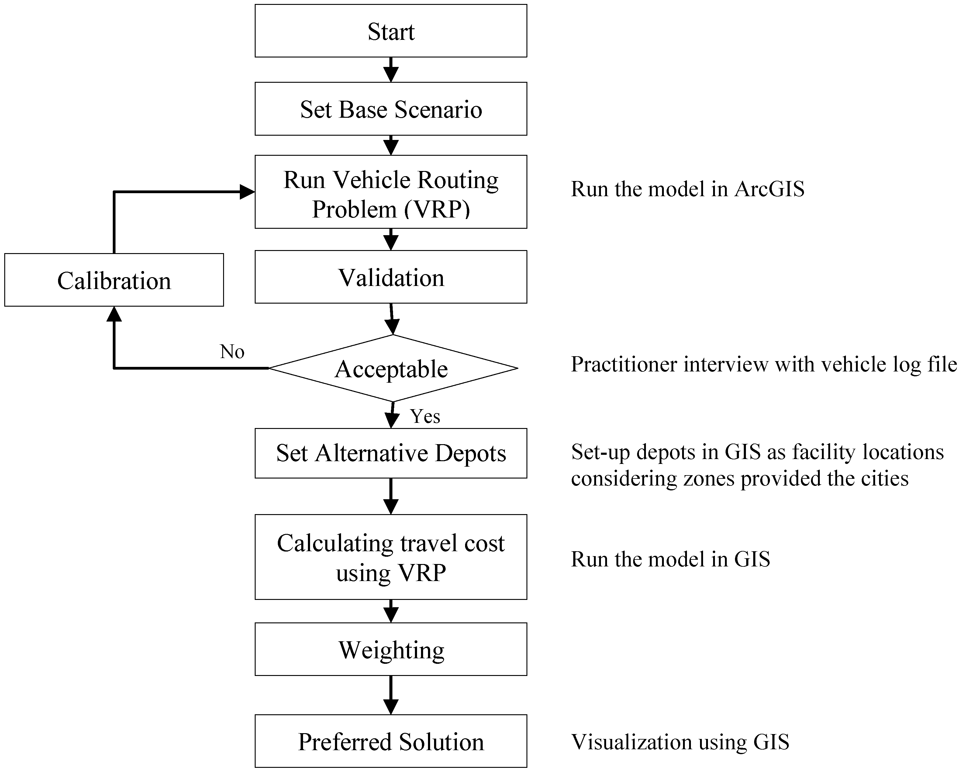
The methodology proposed in this study is described in
Figure 1. First, the authors set the base scenario with current practices. Then the Geographic Information System (GIS) runs the vehicle routing problem using network analysis embedded in ArcGIS
® to build routes for a location in practice. The results were discussed with a dispatcher based on the distributor’s vehicle diaries to validate the base model. Once the model is acceptable, by representing current practices in an appropriate manner, we develop alternative scenario with potential depots. If the base model is not acceptable, the model calibrates relevant parameters in the GIS until it is acceptable.
The GIS repeats the vehicle routing problems with calibrated, fixed parameters from the base scenario to build routes for each location in order to estimate yearly vehicle (
i.e., route) operating costs [
26]. The sets of outputs from 11 potential locations were compared by using a weighted rank method. In the final phase, the preferred solutions with ranks were provided.
The framework was developed to mitigate the complexity of solving vehicle routing and facility location problems, simultaneously, by decomposing the Location-Routing Problem (LRP). The study utilized a Geographic Information System to solve the capacitated vehicle routing problem with time window and hours-of-service rules. The potential locations were weighted based on the total vehicle operating costs. The detailed approaches are in the following sections.
Figure 1.
Research framework of the study.
Figure 1.
Research framework of the study.
3.1. Data Sources
The zone-based location study using vehicle routing problem requires road networks with travel speed and distance, as well as truck traversable information; city development zones from the three cities of Fargo and West Fargo in North Dakota and Moorhead in Minnesota; customer locations and demand; and existing distribution routes and pairs of orders. Non-traversable links from the urban areas were removed from the raw road networks.
TIGER
® road networks were acquired from the U.S. Census Bureau [
27] to make sure all road segments were connected. In addition to the base networks, some road links prohibit trucks in urban areas, so truck routes were identified from cities’ websites. The truck routes were integrated into the base road networks downloaded from TIGER
®. Speed information was acquired from each city’s website and missing information for some links was estimated based on the Highway Capacity Manual [
28]. The City of Fargo provided the development zones through its website (
http://www.ci.fargo.nd.us/). This paper noted that the road links in GIS are asymmetrical, which therefore indicates the difference costs for directions (cij ≠ cji) by considering one-way roads and divided highways. This study also considers the true distance from the true shape of the roads instead of using straight lines with Euclidian distance. Hence, this study uses actual road networks with 223,356 nodes and 244,182 links through 64,265 miles of highways and local and urban roads.
The zone information from the other two cities was provided from city engineers from email requests. The customers and the existing regional distribution center (RDC) were geocoded based on their addresses. The confidential data for the distributor’s routes and demand data were provided from the distribution company. The pairs of orders from customers are sequentially routed, and vehicle drivers plan routes for delivering the orders by considering vehicle capacity (i.e., total demand of each route). The four-year dataset provided by the distributor indicates the distinct routes for Spring, Summer, and Fall to deal with varying demand. The dataset matches the route, customer locations, and sequence for the base scenario.
3.2. Vehicle Routing Problem
The heuristics route construction used in this study follows the Solomon’s route-first and cluster-second approach [
29]. The method establishes one giant tour, with customers scheduled in the route, and then divided into smaller routes. In ArcGIS
®, a tabu search meta-heuristic method is developed extensively in-house [
30]. The embedded VRP in the ArcGIS
® is a superset of the travelling salesperson problem [
31]. The VRP generates an initial solution by sequencing orders, one at a time, until the solution cannot be improved by inserting and moving orders. The algorithm minimizes the overall path costs under the constraints of vehicle (called route) capacities, delivery time windows, driver (called vehicle), and specialties, such as a liquor license, and demand pairs.
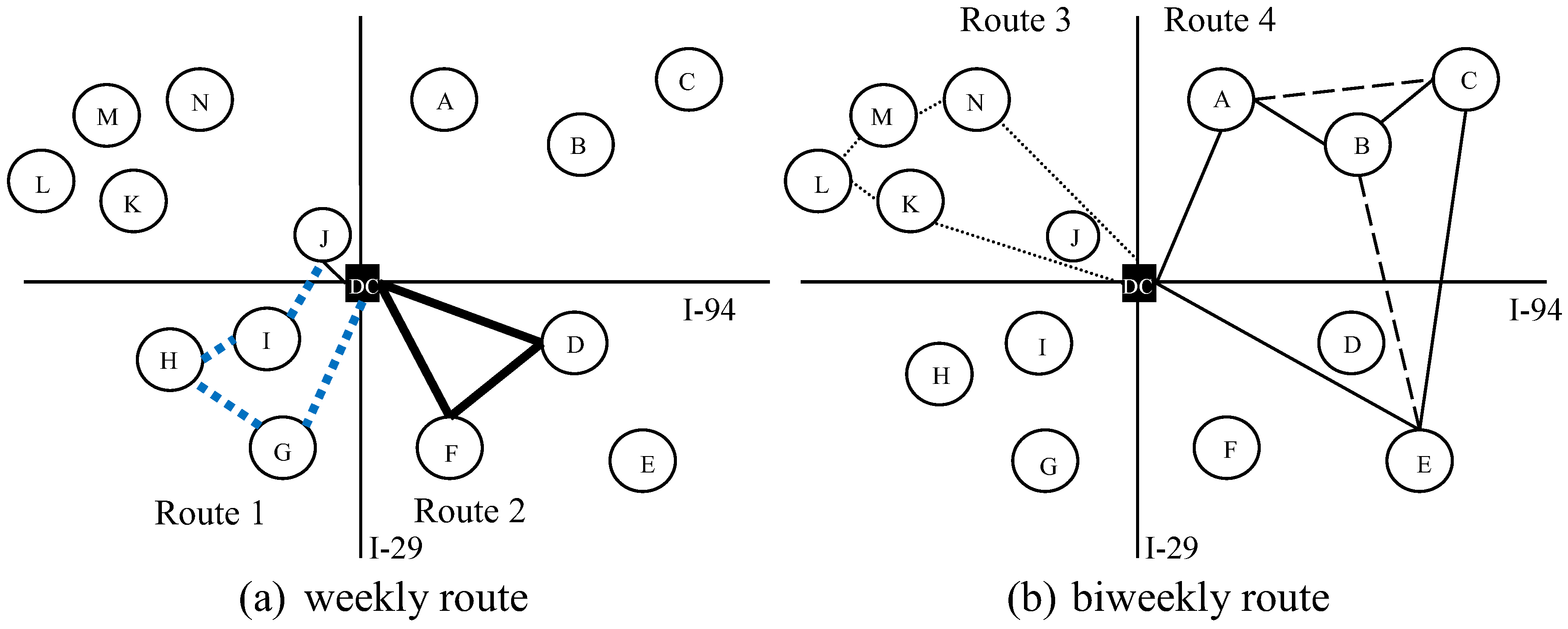
The distributor manages weekly routes and biweekly routes separately, which are fixed depending on demand from customers. The relationship between the distributor and customers also determines the routes. The routes minimize travel distance, and they are subjected to time windows and vehicle capacity, as well as driver’s hours available to drive. For example, two weekly routes are usually located within or near the populated towns: Route 1 is a path of
DC-G-H-I-J-
DC serving customers G, H, I, and J, and Route 2 is a path of
DC-F-D-
DC delivering orders to the customers of F and D (
Figure 2a). The distributor schedules vehicles every two weeks to serve less populated areas (such as Route 3 serving customers K, L, M, and N and Route 4 serving customers A, B, C, and E) (
Figure 2b). Even if a chain of customers for a route is fixed, the sequence of the delivery service is subject to change by the salesman problem in order to minimize the logistics cost of the route for alternative solutions. In
Figure 2b, for example, the series of customers,
DC-A-B-C-E-
DC along Route 3 is served biweekly; however, the sequence of the service of Route 4 would be replaced by the new sequence of
DC-A-C-B-E-
DC to minimize the total vehicle operating cost.
For a base scenario, the sequence of the customers is fixed by the distributor based on the priority and normal orders. The total order quantity of a week represents an aggregation of five days. Drivers keep travel diaries of travel time and distance to report to federal offices. Thus, the distributor can trace the routes of the delivery service and transportation cost derived by vehicle miles traveled and hours during a day and/or a week based on the diaries. This study surveys the weekly travel report to recognize the driving patterns. The travel data is aggregated into a season, and then the seasonal data is utilized to generate vehicle routes to respond to demand change. In the model, a customer will be served by only one vehicle.
Figure 2.
Conceptual vehicle route management for distributing beverage. Note: DC stands for a distribution center called a depot, while each node indicates a customer, called an order facility in ArcGIS®. I-29 is Interstate Highway 29, and I-94 represents Interstate Highway 94.
Figure 2.
Conceptual vehicle route management for distributing beverage. Note: DC stands for a distribution center called a depot, while each node indicates a customer, called an order facility in ArcGIS®. I-29 is Interstate Highway 29, and I-94 represents Interstate Highway 94.
3.3. Validation of the Model
The vehicle routes should be validated before being used for estimating annual routing performance for the alternative locations. Then, the optimized vehicle routes would identify an alternative distribution center location within the feasible zones. First, the sequence of the orders are followed by the current practices, and then compared to the total mileage for travelling the route. Mileage from weekly routes is multiplied by 12 weeks and mileage from biweekly routes by six for comparison to the actual total seasonal mileage. Special routes, which are not regular service routes, and are served by a van, are ignored to avoid noise in the model. The monthly delivery route, which has few orders, is also not captured in the model. Because of a lack of detailed information about the routes and the drivers’ behaviors, validation is done by comparing the seasonally aggregated mileage and each route’s distance and pattern based on visual inspections.
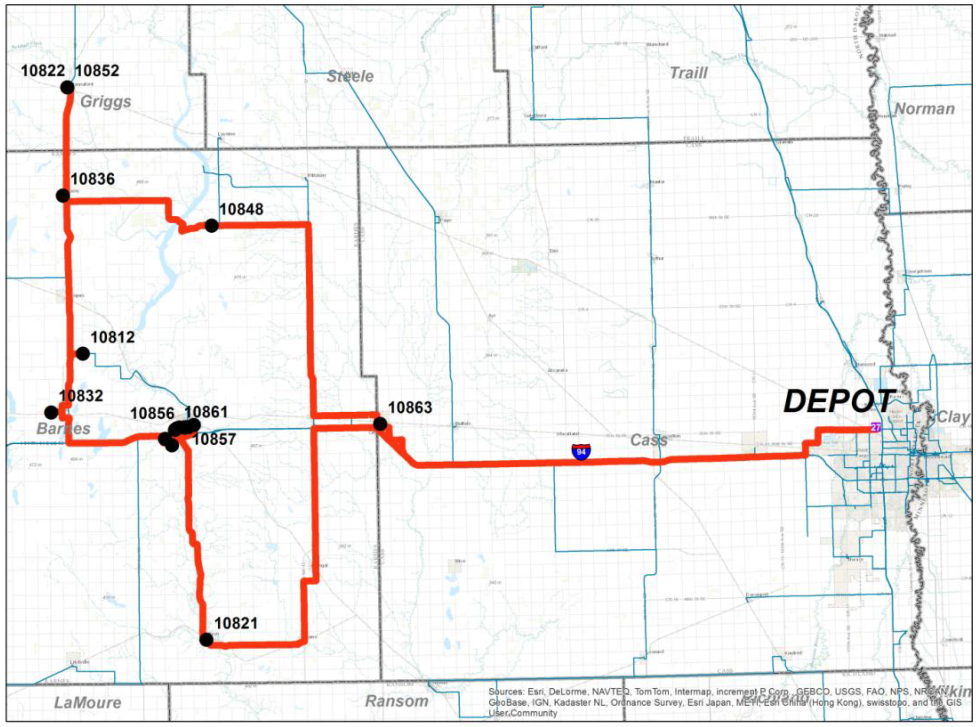
As an example,
Figure 3 shows the optimized sequence of Route 40. Route 40 starts from the Fargo distribution center (visualized as DEPOT) and follows westbound I-94 to serve customers 10812–10863. The vehicle operator delivers orders to customers, 10822 and 10852, and then must drive back to the location of customer 10848 before continuing on to customer 10863. To serve the region, the redundant mileage is required. An interviewee from the distributor confirmed that the patterns of the routes are reasonable and the estimate of the seasonal miles is approximately that of the diaries.
Figure 3.
Route 40 generated by ArcGIS® Vehicle Routing Problem (VRP).
Figure 3.
Route 40 generated by ArcGIS® Vehicle Routing Problem (VRP).
3.4. Location Problem
Total logistics cost for an alternative location is the sum of transportation costs and facility costs. The transportation costs (TCALT) estimation for an alternative location is a combination of vehicle miles travelled (VMT), vehicle hours travelled (VHT), and unloading time (P) from routes, including ordinary travel and extra travel (Equation (1)). The cost of travelled distance and time is assumed to be linear by miles and hours, respectively. The mileage-based costs include maintenance and operating costs of $0.25 per mile, while the travel time-based cost includes the driver’s wage of $15/h as long as it does not violate Hours-of-Service regulation. Due to of the extra service time and longer distance, the driver will be paid additional $5 per hour. The cost for the remains of the extra miles travelled is calculated by the same rate as in normal operations.
where:
: Vehicle miles travelled for route R in normal operation N;
: Vehicle miles travelled for route R for extra distance E;
: Vehicle hours travelled for route R in normal operation N;
: Vehicle hours travelled for route R for extra time E;
: Vehicle maintenance and operation cost per mile in normal operation N (i.e., $0.25/mile);
: Vehicle maintenance and operation cost per mile in extra distance E (i.e., $0.25/mile);
: Driver’s wage per hour in normal operation N (i.e., $15/h);
: Driver’s wage per hour for extra service E (i.e., $20/h);
: Total transportation cost for a candidate location ALT (depot);
: Unloading time through a route R (i.e., 15 min for every stop).
In addition to the transportation costs, the fixed (
FCALT) and variable (
VTALT) facility costs are added to the total logistics costs, thus, the total logistics costs of each location (
TLCALT) can be estimated (Equation (2)) by adding variable utility costs to operate a distribution center and fixed costs to maintain the location and routes. Nevertheless, the land rental (or purchasing) costs and facility operating costs are not considered for this case study since this study proposes the foremost potential locations among all the candidates in the study area.
where:
The location problem compares the alternative locations for a distribution center, thus, the location with the minimum total transportation cost is selected (Equation (3)). The objective function of each alternative location is subject to the total vehicle hours travelled (VHT) and the total vehicle miles travelled (VMT). The total VHT for each trip (route) cannot exceed the consecutive working hours needed for driving the route, and pick-up and delivery because they are subject to regulations dictating of hours of service for drivers [
32]. Those hours of service regulations include a break of at least 30 minutes after 8 hours of driving (Equation (4)). The logbooks should be kept by property-carrying commercial vehicle drivers. In addition to the total VHT rule, the distributor restricts the total VMT for each route for each trip. The sum of VMT in normal operation and VMT in extra miles for each route cannot exceed 300 miles (Equation (5)). A vehicle (V) is assigned to a route, so the total orders from a route (
) should not exceed the capacity of the vehicle, (
: called route capacity in ArcGIS) (Equation (6)). However, the distributor should deliver the weekly demand from a route (
), which will be larger than or equal to the total orders (
) delivered by a vehicle (Equation (7)). The goods can be picked up from a depot (
i = 0), and a vehicle en route does not pick up any goods (Equation (8)). Unloading time was set 15 min for every stop. This paper does not include the pick-time into the driving hours because this study assumes most of vehicles controlled by the company to have similar loading times and waiting times to be dispatched.
Either a commercial zone or mixed industrial zone can be used for an alternative location for a potential distribution center. Fifty-one square mile zones were selected from three cities as candidate locations. Then the centroid of the zones is considered as an alternative location for a potential location.
3.5. Business Growth and Dynamics
As the business grows, the capacity of the vehicle fleet and warehouses are also in need of expansion. Beverage consumption is closely related to the population in the towns. To address this growth and increasing demand, this study uses a simple growth rate of 1% per year for an unknown time period. The population growth can be found from Departments of Commerce in North Dakota and Minnesota. Long-term forecasting is taken into account in decisions related to investments and potential locations of distribution centers.
4. Results and Implications
Based on the existing distribution center, the total transportation costs estimated show $397,520 for 203,528 miles travelled (
Table 1). The base location’s average transportation cost to maintain the existing routes is $29,366 for 15,241 miles travelled on average. All but one other alternative location result in higher transportation costs than the transportation costs of the base location. Alternative G has a projected annual transportation cost of $396,103 and total miles travelled of 202,577.
The output in
Table 1 was based on two groups of measures: annual transportation cost and mileage for all vehicles in the fleet and average transportation cost and mileage per route. This method was conducted to ensure that every route was individually accounted for. This allowed us, not only to validate the model, but also to deal with individual exceptions in the route, wherein a route serves a different number of customers during different seasons. For every alternate location, annual miles per route per season are calculated. Miles per route per season are aggregated to arrive at total annual miles for a candidate location. Since a route serves a different frequency of deliveries with the change in season, it was critical to account for it in order to conclude total annual miles per route. This approach was actually helpful in verification of many routes initially when compared for observed
versus calculated.
The transportation cost and travel distance are ranked in
Table 2. The four measures ranked are averaged to find the best among the 10 candidates, based on the simple average ranking method. The average rank can be expressed by
, where
k is a criteria and
r is ordinal rank in the set of criteria
k. The minimum value of the average rank has a higher opportunity to be chosen. From the summary (
Table 2), Alternative G in Fargo is preferred to the Base location, while Alternative A is ranked with very low preference in Fargo. In other words, new location G will provide better performance by reducing annual costs by $1417 and annual miles traveled by 952 miles per year. Based on the saving, the logistics planner will not move from the Base location to the G location if the company cannot save more than $1417 from the location operating costs per year. In Moorhead, Alternative H ranked 3.8, which is not highly preferable. It is noteworthy that the goal of the study was to identify potential locations considering total transportation costs and land use plan from the three cities in the study area.
Table 1.
Cost and distance analysis for current and potential candidate locations.
Table 1.
Cost and distance analysis for current and potential candidate locations.
| Alternative | Annual for all vehicles in fleet | Average per route |
|---|
| Transportation cost ($) | Travelled miles | Transportation cost ($) | Travelled miles |
|---|
| A | 421,613 | 216,445 | 30,819 | 16,014 |
| B | 403,431 | 207,513 | 29,664 | 15,451 |
| C | 416,996 | 215,311 | 30,712 | 16,053 |
| D | 405,172 | 208,537 | 29,882 | 15,577 |
| E | 400,460 | 205,738 | 29,468 | 15,334 |
| F | 414,556 | 212,744 | 30,253 | 15,714 |
| G | 396,103 | 202,577 | 29,287 | 15,186 |
| H | 401,109 | 205,343 | 29,663 | 15,393 |
| I | 411,003 | 210,716 | 30,099 | 15,622 |
| J | 416,341 | 213,964 | 30,603 | 15,925 |
| Base | 397,520 | 203,528 | 29,366 | 15,241 |
Table 2.
Ranking method for multi-criteria location decision.
Table 2.
Ranking method for multi-criteria location decision.
| Alternative | Annual | Average per route | Average rank |
|---|
| Transportation cost ($) | Travelled miles | Transportation cost ($) | Travelled miles |
|---|
| G | 1 | 1 | 1 | 1 | 1 |
| Base | 2 | 2 | 2 | 2 | 2 |
| E | 3 | 4 | 3 | 3 | 3.3 |
| H | 4 | 3 | 4 | 4 | 3.8 |
| B | 5 | 5 | 5 | 5 | 5 |
| D | 6 | 6 | 6 | 6 | 6 |
| I | 7 | 7 | 7 | 7 | 7 |
| F | 8 | 8 | 8 | 8 | 8 |
| J | 9 | 9 | 9 | 9 | 9 |
| C | 10 | 10 | 10 | 11 | 10.3 |
| A | 11 | 11 | 11 | 10 | 10.8 |
5. Conclusions
This paper investigated potential locations for beverage distribution in Eastern North Dakota and Western Minnesota. For the analysis, the study used geospatial tool for solving vehicle routing problem to estimate the total transportation costs for each alternative location. Ten candidates were considered from commercial and industrial zones in the cities of Fargo, West Fargo, and Moorhead for potential locations to site a distribution center. The candidate locations were analyzed to determine which site minimizes transportation cost and travel miles regarding truck routes.
The study found that most attractive locations for distribution center are close to the intersections of major highways due to accessibility and decrease of the total transportation costs. From the analysis, the study recommends locating a distribution center at alternatives G, E, and H, based on the average ranking method.
In the travel cost and time analysis, other costs for land acquisition, maintenance, and local and special taxes are not considered in this paper. In addition to the cost, ease of access to the loading ramp can also be an important factor for truck delivery. Currently, only the sequence of customer visits for a particular route is optimized. With a new location, it may be helpful to optimize the assignment of customer locations to various truck routes. The current theoretical inefficiency of miles travelled without such optimization should be compared with ability to maintain or gain customers from current routes between drivers and customers. The aforementioned stochastic components of unloading time and break time should be carefully included in the future research, since hours for resting and loading/unloading time will limit the driver’s actual working hours and influence critical safety issue.
The method in this study can easily be applied to distribution companies for long-term and mid-term strategic planning to find cost effective locations. While the authors utilized a geospatial tool, embracing advanced vehicle routing algorithms, the paper provided a research framework to provide a practical approach by decomposing the location routing problems. By doing so, the paper proposed practical research method with a case study while considering time window of the delivery, vehicle capacity, Hours-of-Service regulation, and local governments’ land use plan.


