Real-Time Three-Dimensional Imaging of Soil Resistivity for Assessment of Moisture Distribution for Intelligent Irrigation

1076 Carol Lane, Lafayette, CA 94549, USA
Hydrology 2017, 4(4), 54; https://doi.org/10.3390/hydrology4040054
Submission received: 24 October 2017
/
Revised: 17 November 2017
/
Accepted: 17 November 2017
/
Published: 20 November 2017
Abstract
:An affordable standalone sensor that can provide volumetric information on soil moisture distribution in real time was developed and tested for potential application in irrigation control systems. The moisture content of soil is reconstructed tomographically from electrical resistivity measured between multiple pairs of electrodes, which are installed on two opposite sides of the soil volume. The measurement of relative moisture content reconstructed from the measured resistance values demonstrated in this paper requires a simple, in-situ, two-point calibration (for dry and wet soil conditions) after electrodes are installed in place. This calibration has to be repeated once the soil conditions, such as salinity or fertilizer content, are altered as the season progresses. Historical data collected over a 12-month period can be stored locally or transferred over a wireless network at given intervals or in real time. Although existing single-point sensors can provide more accurate measurements of soil moisture, knowledge on the three-dimensional distribution of moisture around plant roots should allow substantial savings of precious fresh water resources and more intelligent multi-channel irrigation systems. The same system can possibly be extended to estimation of fertilizer distribution.
1. Introduction
Hunger, one of the most prominent problems in the world today, is primarily caused by a shortage of fresh water [1]. This problem is especially severe in third-world countries and regions with low rainfall or that are prone to severe droughts. For example, the most recent California drought (2013–2016) vividly demonstrated the importance of fresh water conservation [2,3]. The state’s large agricultural industry was most heavily impacted by the weather abnormality [3], with some crops being completely deprived of irrigation water. The expense of lost plants forced many farmers to reconsider their irrigation methods. The use of traditional sprinkler systems is accompanied by substantial evaporation and watering of unused soil regions. In response to this, some farmers have implemented subsurface drip irrigation systems, which can save up to 25–50 percent of water [4,5,6,7,8]. Furthermore, significant optimization of water use can be achieved by knowing the exact time and amount of needed water, as well as the specific location of soil that requires irrigation. Recently, various novel methods for soil moisture measurement have been developed [9,10], which can be used for the intelligent irrigation control systems. In order to measure the soil moisture content, different physical properties of soil may be analyzed, such as the dielectric constant, resistivity, thermal conductivity, neutron absorption and others. For example, dry soil has a dielectric constant of 2–5, while water has the dielectric constant equal to ~81 [11,12,13]. Because of this large difference, the most accurate moisture sensors use it to determine the moisture content [9,10,11,12,13]. Time Domain Reflectometry (TDR) proved to be one of the most accurate measurement techniques [11,12,13]. This method has little dependence on soil type and thus does not require calibration for every new soil. Another parameter which can be used for estimation of moisture content is the thermal conductivity of soil, which noticeably changes when moisture content is changed but it is also affected by other factors such soil composition. Neutrons are heavily scattered by hydrogen contained in water and, at the same time, they easily penetrate dry soil [14]. However, neutron-based sensors are impractical for wide use in the field.
Another soil parameter that can be used to measure moisture content is soil resistivity, which typically varies between 10 and 1000 Ω·m [15]. The deficiency of this parameter is in the fact that resistivity greatly varies between different types of soils and can be affected by added substances, such as fertilizer. Resistivity can also be affected by soil salinity, which can change as the season progresses. It can also change with temperature, as resistance increases dramatically at temperatures close to or below freezing. The resistance of soil was reported to change by a factor of ~2.5 from the month of February to May [16]. However, the resistance did not change that much during the months of crop production when irrigation is required. If necessary, the variation of resistance with temperature can be corrected to current temperature after proper calibration for a particular type of soil [16,17,18]. However, there are several reasons why soil resistance is still used for the measurement of soil properties. The capability of DC signal to penetrate large distances in soil, for example, is widely utilized in soil resistivity measurements in geophysical research when implemented in electrical resistivity tomography (ERT) systems [19,20]. Resistivity measurements also involve relatively simple DC electronics, rather than expensive high frequency circuits.
Most traditional soil moisture sensors provide single-point information on moisture content and remain somewhat expensive for wide use in irrigation control systems. A wide range of commercially available single-point (and single line) sensors exists at the present time. However, irrigation can be made significantly more efficient if volumetric information on soil moisture distribution is known. The volumetric measurement of soil moisture has already been demonstrated in principle in a laboratory-based prototype system (e.g., as described in references [21,22,23] with a TDR sensor [24]), or in a permanently installed system of multiple sensors on a 3D grid as in reference [25]. However, such systems still remain less practical compared to single-point measurement of soil moisture content and do not have wide use outside of research installations.
In this paper, a method of volumetric measurement of relative soil moisture content is introduced together with a possible hardware implementation in a standalone, easy-to-install system. It is not intended to replace or outperform existing soil moisture sensors but rather to provide a low-cost alternative for volumetric measurement of moisture content around plant roots. Despite many deficiencies of the present system, such as its sensitivity to the salinity of soil, temperature, or porosity, this system can be an attractive, affordable alternative to existing sensors, with a multi-unit implementation in the field. Moreover, the inaccuracy of measurement due to variation of factors other than soil content can be corrected by the correlation of sensor volumetric data with an accurate single-point TDR sensor (e.g., as it has been demonstrated in a system described in reference [21]).
The recent development of inexpensive microelectronics enabled fast data acquisition and processing, which are utilized in the sensor described in this paper. The system uses multiple measurements of resistance to reconstruct the relative three-dimensional distribution of moisture in real-time. Although the system is not as precise as many single-point sensors, its volumetric output, simplicity and low cost can be advantageous for wide use in precision irrigation. The system is capable of wireless data transmission, pairs all measurements with exact time and location from a GPS signal, can store large amounts of historical data (~12 months as defined by the capacity of the storage memory), features one-button calibration, automatically adjusts the accuracy of resistivity measurements for different types of soil and, most importantly, provides real-time 3-D imaging of relative soil moisture content. By using this system, farmers can volumetrically optimize their irrigation methods, applying water to specific locations within the root system of various plants. Through the virtue of the system’s affordability (can be less than 10 dollars in mass production), multiple units may be placed throughout the field to enable the most efficient irrigation. In addition, analysis of historical data allows for optimization and planning of future watering techniques.
2. Materials and Methods
2.1. System Design
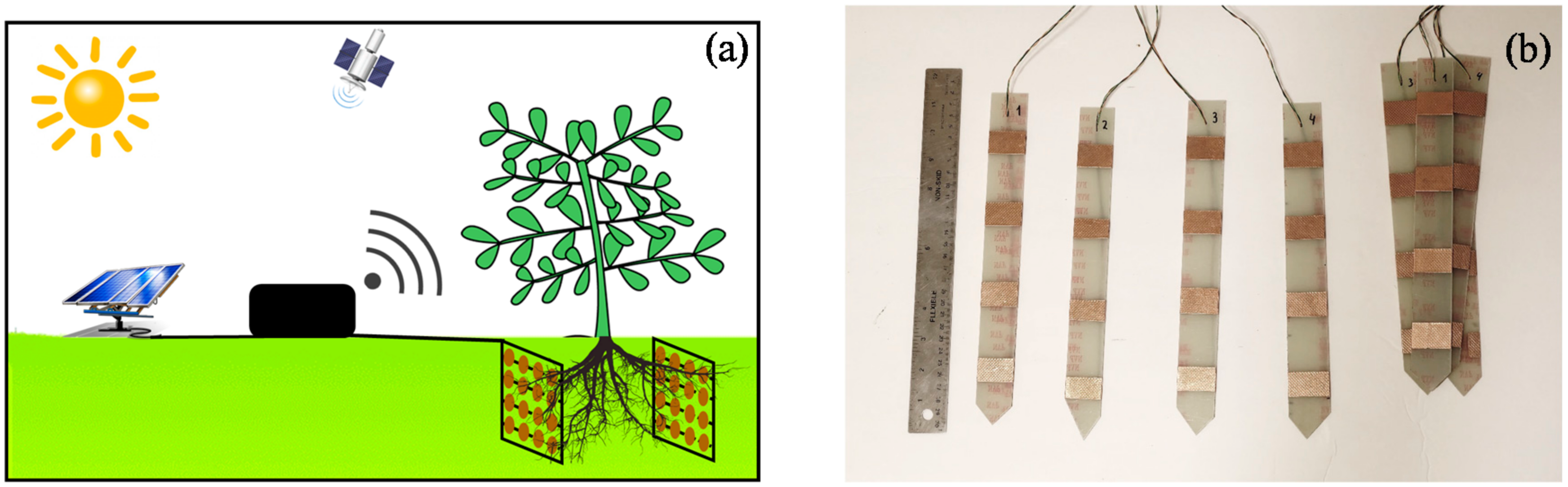
In contrast to single-point moisture sensors, the present system measures volumetric relative moisture distribution. This is done by measuring soil resistance between multiple points located on opposite sides of the tested volume, followed by data processing, which reconstructs the three-dimensional moisture content. Similar to conventional tomographic imaging in which transmission through the sample is measured at different angles [26], the present approach effectively probes resistance throughout the volume at various angles. For this reason, two sets of electrodes need to be placed on opposite sides of the tested volume as shown in Figure 1. The volumetric distribution of soil moisture content is determined from soil resistance. Two sets of electrodes are placed at opposite sides of a plant root. Resistance between all pairs of electrodes is measured multiple times per second. Measured data paired with exact time and location from a GPS signal is transferred via a wireless connection and simultaneously stored locally on an SD card. Electrode arrays can compose different geometries, including a rectangular, circular, or other grids. One example of an easy-to-install electrode array is shown in Figure 1b, which consists of individual flat rods, each containing four electrodes. Corrosion-resistive metals should be used for electrode plating, similarly to other existing soil moisture sensors. Due to their simple construction, the electrodes can also be disposable and can be recoated at the start of each season. The placement of sensors relative to each other and to the tested volume determines the measured values of resistance. Therefore, separate electrodes should be installed at nearly equal intervals but not to a millimeter accuracy. A very accurate alignment of electrodes is not needed and manual installation is sufficient for the operation of present system.
After acquiring resistance values, the solar-powered control unit pairs these values with the exact time and location retrieved from a GPS signal, which can be used to locate the position of a particular sensor if multiple systems are used throughout the field or if historical data is analyzed for a sensor that was moved around the field. Data is stored locally on an SD card and sent via a wireless connection. The system continuously self-adjusts for the most precise measurements in the given medium, as described in Section 2.2.
Theoretically, the system is capable of measuring the quantitative moisture content with appropriate calibration. However, for practical irrigation purposes, it is not necessary to know the exact value of moisture content. It is important to make a decision on where and when water should be applied and when irrigation should be stopped. If information on the moisture content at a single point is sufficient for irrigation control, the present system does not have any benefits compared to accurate sensors, such as ones based on the measurement of the dielectric constant. However, when real-time volumetric information is used to optimize the irrigation protocol for a large field (thus requiring many sensors) the present affordable (and yet not very accurate system) can be an attractive alternative to the existing sensors. Compared to single-point sensors, the present system can provide volumetric information, which would otherwise require installation of many single point devices into the volume of the soil, not to its periphery, as in present system. The number of devices to be implemented per unit area has to be decided based on how much variation of moisture content is expected in a particular field. The deficiency of resistivity measurement in the present system limits its practical use to the measurement of relative moisture content and thus requires in-field calibration.
For a particular soil, calibration can be carried out to determine the resistance of dry soil and the resistance of soil with an adequate moisture content for a particular crop. The user has to decide what the state of dry soil is (and record those values with a press of a button), as well as record the resistance of properly irrigated soil. The frequency of this recalibration is currently determined somewhat subjectively, unless a correlation to an absolute moisture content sensor is implemented. With these two values, the measurement of relative moisture content becomes sufficient for irrigation control. It is to be determined for a particular soil and a particular field how often the calibration procedure has to be performed in order to provide sufficient accuracy for the irrigation system and remains to be a subjective decision. Correlation with an accurate single-point sensor can be utilized as well for more precise criteria on how frequently the system needs to be re-calibrated. Since all measurements are performed in real-time, it will be known when watering should be stopped. The resistance measured between every pair of electrodes on opposite electrode arrays is used to reconstruct the volumetric distribution of moisture.
The system switches between different pairs of electrodes through the use of electronic multiplexers (as shown in Figure 2). The soil resistance is found from the voltage drop across resistor Rtest,—as shown in Figure 2a—for one pair of electrodes. Figure 2b shows the principle of resistance measurements carried out by multiple electrode pairs. A voltage drop across the programmable resistor (Rtest) is measured by two electrodes from opposite electrode arrays that are connected to the circuit by multiplexers, which in turn are controlled by shift registers. The use of shift registers enables a large number of electrodes to be controlled by a single microcontroller. The programmable resistor is automatically optimized to improve the accuracy of the results. Resistance Rsoil (i,j) between all pairs of electrodes is measured multiple times per second. To minimize the number of necessary microcontroller pins, a series of shift registers is used to set necessary signals for the control lines of multiplexers. Therefore, the system with a single microcontroller is scalable to large arrays, as a single microcontroller is able to sequentially switch between many electrodes.
To measure the resistance between a given pair of electrodes, the voltage drop across resistor Rtest is measured by an analog to digital converter (e.g., the one available on an Arduino microcontroller board) as shown for one pair of electrodes in Figure 2a. The resistance of the soil between a pair of electrodes is calculated according to the equation:
where V1 is the measured voltage drop (in volts) across the test resistor and Vin is the input voltage (5 V in our case). The small (several volts) voltage drop across the soil volume and the application of current for a short period of time should preclude electrolysis or charging problems within the measured volume [27]. It is also very easy to switch the polarity in such a system by implementing an electronic relay. To optimize the accuracy of measurements, a programmable resistor is used for Rtest, as described in Section 2.2. All resistance measurements can be performed in a fraction of a second, followed by real-time algorithmic reconstruction of volumetric moisture distribution.
2.2. Optimization of Measurement System: Automatic Sensitivity Adjustment
The accuracy of Rsoil measurements depends on the value of the test resistor Rtest. The value of the test resistor needs to be optimized for specific soils and moisture conditions, which can change significantly in different environments. The system automatically adjusts Rtest to an optimized value according to the following procedure: at a given time, the resistance value between all pairs of electrodes varies from Rsoilmin to Rsoilmax, which results in measured values V1 of Equation (1), changing between Vmax and Vmin (all in volts). To digitize the array of resistances most precisely, this range of measured voltages should be maximized:
The range of measured voltages will be maximum when 𝐹′(𝑅𝑡𝑒𝑠𝑡) = 0:
Since the resistance is only measured in positive values and has only one critical point for the positive values of the argument, the optimal value of Rtest can be found from the following equation:
At the beginning of each measurement cycle, the present system determines Rsoilmax and Rsoilmin and calculates the optimal value of Rtest for the present conditions according to Equation (4). If the optimal resistance value is different from the current one, the microcontroller adjusts the nonvolatile programmable resistor Rtest to that value, enabling the most accurate measurement of soil resistance.
2.3. Volumetric Reconstruction of Moisture Content
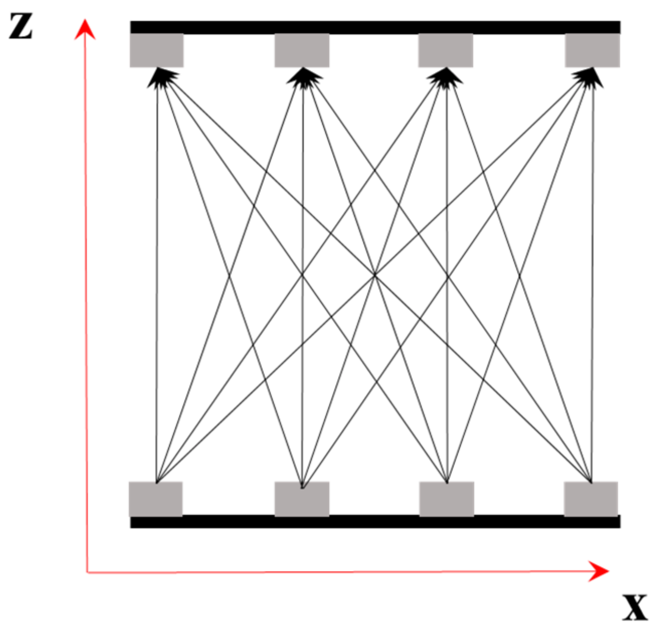
Reconstruction of bulk resistivity values from the resistances measured between the electrode pairs requires an inversion procedure. A set of 2-dimensional inversion procedures was implemented by Brillante et al. [25] to form a quasi-three-dimensional matrix, allowed by the multiple sets of electrodes installed through the entire volume. In the present system, the electrodes are placed only on opposite sides of the volume and therefore two-dimensional inversion cannot be implemented. A full 3D inversion procedure was not available in the present study, although in the future it can be developed by an adaptation of the existing Geotomo software tool [28]. A simplified, fast reconstruction method was applied in the present study, which represents the location of moisture in the studied volume (although not as precisely as in accurate analytical inversion). During approximated reconstruction, it is assumed that current flows between two electrodes in a straight line (as shown in Figure 3), although the current flows through the entire bulk of soil. The simulation results of current flow presented in Section 2.3.1 demonstrate the sensitivity of the linear approximation to the location of the wet region along the path between two electrodes. After all resistances between all pairs of electrodes are measured, the reconstruction algorithm is implemented before the system continues with next set of measurements. During the reconstruction procedure, the volume between two arrays of electrodes is divided into virtual cells with assigned indexes (k, l, m). For a given pair of electrodes, the algorithm determines which cells are crossed by a virtual “current line” connecting electrodes. The resistance measured between that pair of electrodes is then equally divided between the subset of cells that are crossed by the virtual line. This process is repeated for all electrodes (256 pairs in present 4 × 4 electrode system). As a result, multiple values of resistance are assigned to each cell which can be crossed by multiple lines. Following that, an average resistance value in each cell (k, l, m) is calculated (averaged over all crossings over a particular cell). These values are sent out and stored on the local SD card. The resulting three-dimensional distribution of resistances is correlated to the volumetric distribution of moisture content, as soil becomes more conductive with increased water concentration (as shown in Section 3.1).
The absolute values of moisture content can be calibrated for any particular type of soil (as shown in Section 3.1). Alternatively, in practical use, irrigation control system need to determine when soil is dry and should be irrigated, as well as when to stop irrigation. The decision on when to start watering in a particular irrigation pipe and when to stop it does not require knowledge of resistance values but can rather be based on the comparison of the current resistance to the resistance of dry and wet soils. After installing the electrode sets, the user must do only two simple calibration measurements to find the resistance of dry soil and wet soil. With that simple calibration, all results can be shown in real time as a ratio of current values to the resistance of dry soil. The calibration has to be repeated at certain intervals, depending on the variation of soil salinity as the season progresses, application of fertilizers and other factors. After the user decides what soil conditions correspond to dryness, the program remembers these conditions as a baseline. Similarly, it can be defined when soil is properly irrigated. Another alternative solution for the inaccuracies of resistance-based volumetric measurements can be the correlation of measured values with the measurements of one accurate single-point sensor which is not affected by environmental and soil composition factors, such as a time domain reflectometry device.
2.3.1. Computer Simulation of Electrical Current Flow Pattern. Validity Check of Linear Approximation Used in Reconstruction of Volume Resistivity
The approximated procedure used for the tomographic reconstruction of volumetric distribution assumes that most electrical current flows along the linear path connecting two electrodes. A computer simulation model of three-dimensional current flow is used to estimate the variation of effective resistance between two electrodes in two cases, when a wet soil region is placed in a direct path between two electrodes and when it is placed away from it, as shown in Figure 4a. The Computer Simulation Technology Studio Suite software is used for the simulation. An electroquasistatic solver in the low frequency domain of the CST Studio Suit with a tetrahedral mesh (with an adaptive mesh refinement) was used for the simulation of the soil region consisting of dry soil with an inclusion of a wet region. A cube of uniform conduction (representing a dry soil) contains two metal (copper) electrodes located on the opposite sides. A smaller volume with a higher conductivity value is placed in a direct path between two electrodes (as shown in Figure 4b), as well as farther away from the direct line between the electrodes (Figure 4c) and no wet region is modeled in Figure 4d. The resistance between the two electrodes is calculated to be 15.312 kΩ for case (b), 16.33 KΩ for case (c) and 16.498 KΩ for case (d), respectively (as shown in Figure 4). For a cube containing only wet soil, the resistance would be measured as 164 Ω. Cross sections of the simulated volume include arrows that indicate the value of conduction current density (Figure 4b,d). It is demonstrated that in the first case, a larger conduction current (and thus lower resistance) should be measured providing some sensitivity to the location of the wet soil within the cube. Although these results do not explicitly confirm that linear approximation can be used for the tomographic reconstruction, the experimental results presented in the next section demonstrate the capability of the present device to visualize the location within the volume that has higher moisture content due to the application of water.
3. Results
3.1. Dependence of Soil Resistance on Moisture Content: Calibration with the Present Device
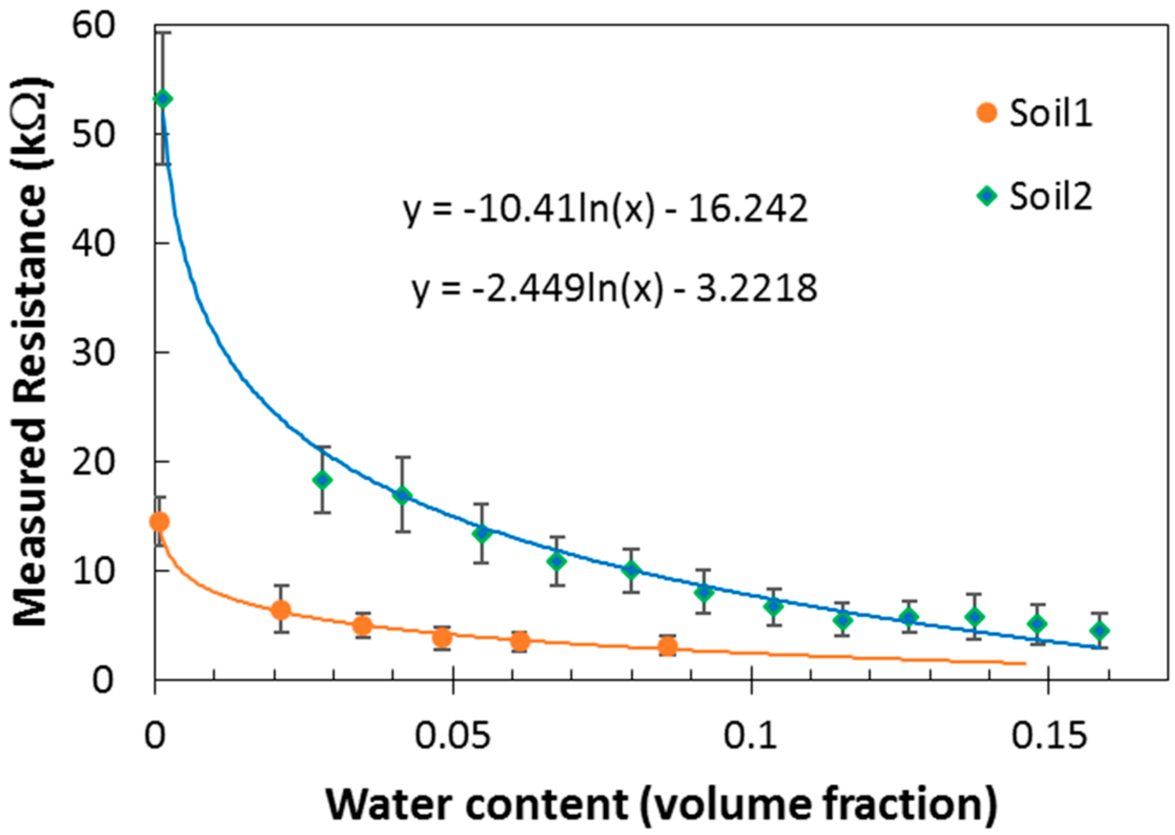
The resistance of soil is known to have a logarithmic relationship with the moisture content [15]. Different types of soil vary in their resistance values depending on their consistency, concentration of salts, granularity and other factors. The dependence of soil resistance on moisture content was calibrated by the following procedure for two types of soil. Soil 1 used in the present study was a general Garden Soil mix available from garden stores (three parts organic matter, such as peat, humus or sawdust; one part combination of sand, perlite, vermiculite; one part sphagnum peat moss). Soil 2 had density of 0.8 g/cm3, porosity of ~60% and field water capacity of ~12%. A pair of electrodes was installed at a fixed distance of 30 cm in a dried soil sample and its resistance was measured. This measurement was assumed to correspond to a nearly zero moisture content (Soil 1 was dried for a period of ~3 months while dispersed into a thin layer). Subsequently a known amount of water was mixed uniformly throughout the entire soil volume and resistance was re-measured after each step (as depicted in Figure 5). The relative error of measured values remained nearly constant (at ~20% level of the measured resistance) within the range of 1–100 kΩ due to the fact that Rtest values were adjusted automatically for each measurement, as described in Section 2.2. A logarithmic equation describes the measured values of resistance for both types of soils. Although quantified water concentration can be reconstructed from the measured resistances, in field applications, only two points are needed for the operation of the present device, as mentioned earlier. Other, more accurate single-point measurement techniques (e.g., the ones based on the measurement of the dielectric constant [9,10,11,12,13]) can be used to correlate the relative volumetric values obtained from the present system with the absolute moisture content obtained at a particular point in the soil.
3.2. Device Scalability: Limits on the Geometrical Size of the Measured Volume
The present system has a limited range of resistance values which can be measured by the Arduino microcontroller with its finite internal resistance. As the distance between the electrodes increases, the measured resistance of the soil increases, limiting the maximum distance between the electrodes which can be used in the present device. At the same time, as the distance between the electrodes increases (e.g., in case of a plant with larger roots) the area of electrode can be increased proportionally, maintaining the measured resistance within the optimal range of values (typically 1–100 KΩ). As the area of the electrodes increases, the spatial resolution of the present system decreases, while the number of virtual cells remains constant since the same number of electrodes is used. Figure 6 demonstrates the possibility to optimally adjust the configuration of electrodes to an optimal value, which allows for an accurate measurement of resistance between the electrode pairs. These results demonstrate that in order to keep the resistance in the same range required for accurate measurements, an increase in electrode separation can be compensated by an increase of the electrode area. The linear dependence of measured resistance on the inverse value of the electrode area confirms that soil moisture distribution can be effectively measured for various plants and crops by the present system. These results indicate that volumes as large as 1 cubic meter can be measured by the present approach, when the electrodes are scaled properly. It should be noted that the spatial resolution of the system scales with the number of electrodes and their size. Since larger volumes require larger electrodes to be used in order to maintain measurable resistances, the spatial resolution of the present system should remain nearly constant in terms of measured pixels/voxels. For a system of two pairs of 4 × 4 electrode arrays, for example, 64 volumetric voxels can be reconstructed and possibly more with the future development of more sophisticated inversion procedures. Thus, in case of smaller separation of electrodes, the absolute spatial resolution can be higher, as each pixel of the reconstructed volume will also be smaller.
3.3. Dynamics of Water Penetration: Real Time Visualization of Moisture Content through Measured Resistance
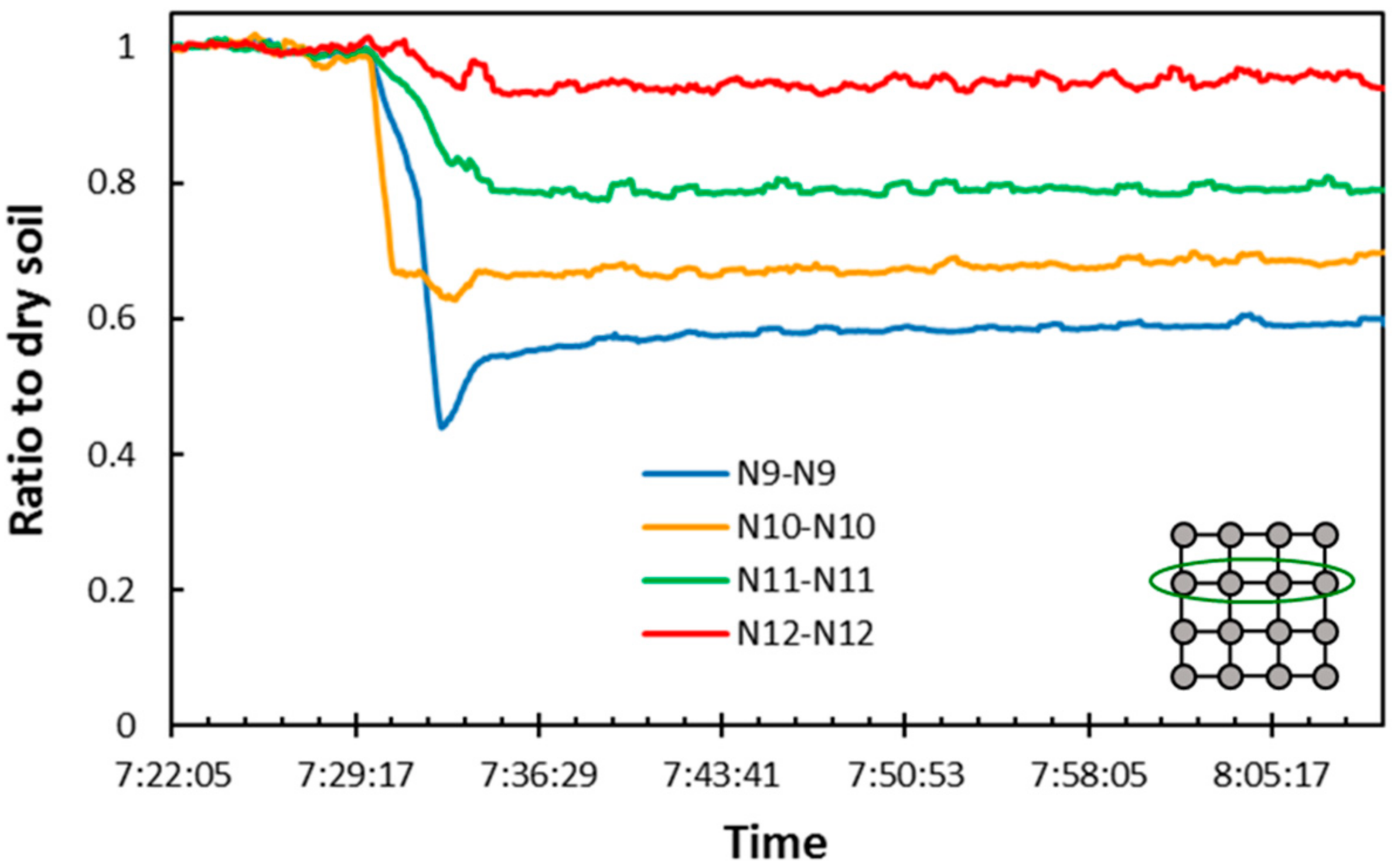
The operation of the system is demonstrated with the measurements of liquid penetration during watering, which was applied to one corner of the tested soil region (as schematically depicted in Figure 7). The measurement of resistance between opposite pairs of electrodes was conducted cumulatively over a period of several months for a soil volume in a laboratory environment, while the temperature was maintained within the +18 °C to +24 °C range. No field tests of the present system were performed. The present paper describes the concept of the system rather than a device ready for a field use. No substantial variation of measured resistances was observed due to charging or electrolysis effects, which (if existed) were below the sensitivity of present system. The variation of relative soil resistance during watering is shown in Figure 8, Figure 9 and Figure 10 as a function of time. Even before the application of water, various electrode pairs exhibited different resistance measurements, as the electrical connection between the electrode and the neighboring soil, as well as local conductivity of the soil itself, varied from one electrode to another. In order to account for these irregularities, a ratio of present resistance values to the resistance of dry soil is calculated during the real-time reconstruction of the moisture distribution. Due to this normalization process, most unaccounted environmental or instrumental factors apart from the application of irrigation are eliminated as the causes of the variation in measured resistance values.
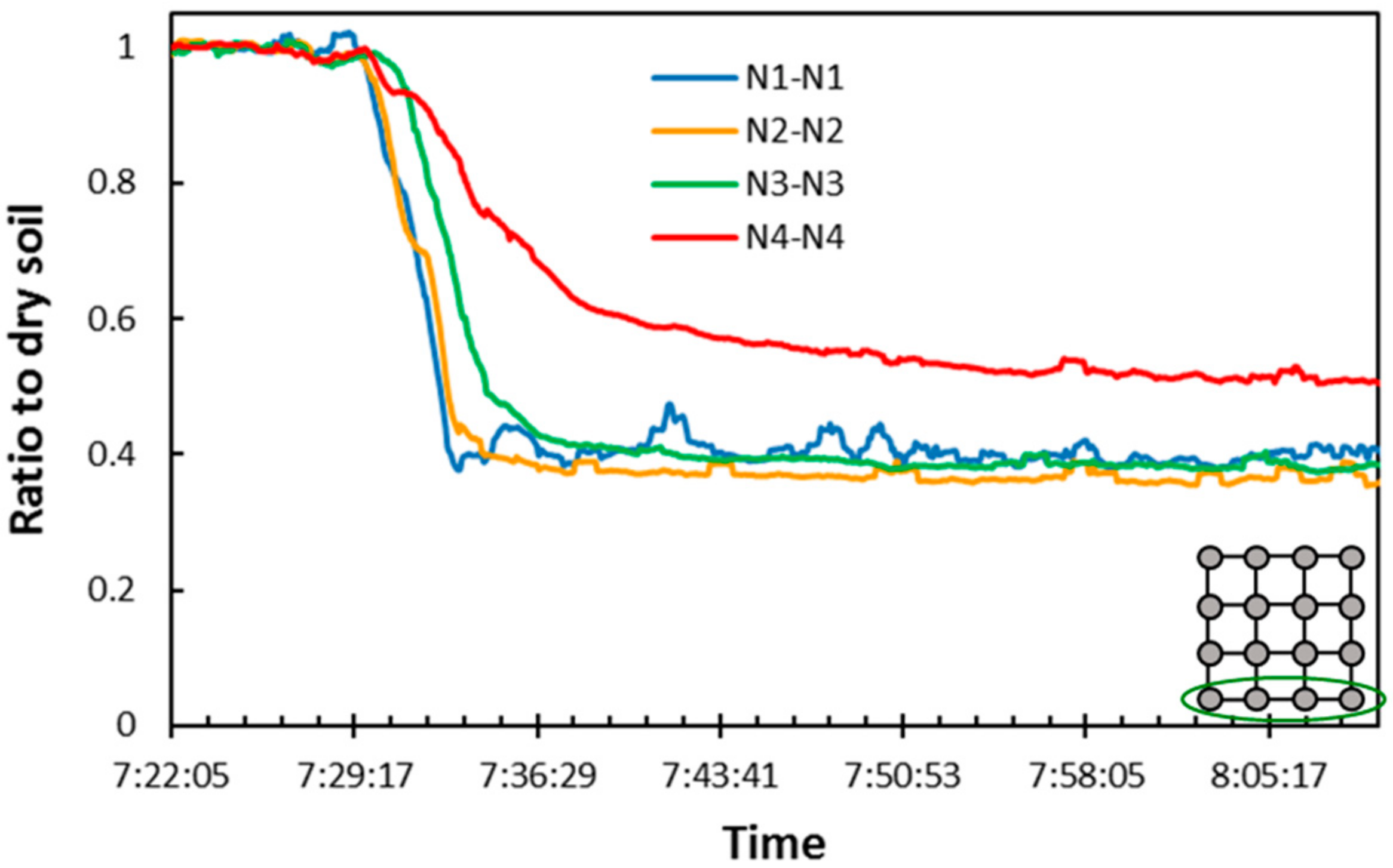
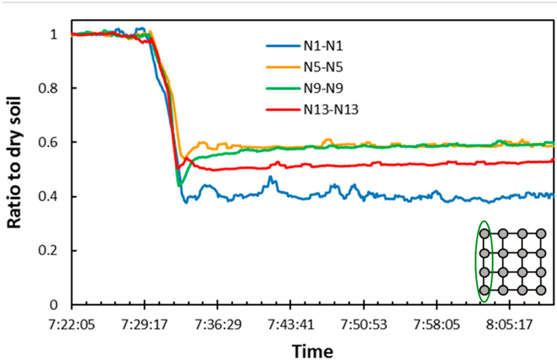
As shown in Figure 8, Figure 9 and Figure 10, after the application of water, there was a substantial change in soil resistivity measured by electrode pairs that were located close to the corner to which the water was applied (electrodes #1, #5, #9, #13). It is interesting to note that water temporarily formed a pocket near electrode #9 (Figure 8), after which it streamed downward toward the bottom of the container. A small change in resistance was observed for electrode pair #11 and almost no change in resistance was observed for electrode pair #12, which was the farthest from the water source. As expected, the water concentrated at the bottom of the container. As seen in Figure 9 electrode pairs #1–3 measured smaller resistance values, while electrode #4, which was the farthest from the water source, measured larger resistance values. At the same time, the resistance measured by pairs #1, #5, #9 and #13 dropped quickly after the application of water above that column of electrode pairs (Figure 10). A distinct difference in resistance near the top and bottom of the soil volume was observed, as most water either stayed at the top of soil or propagated towards the bottom of the sampled volume.
A long-term process of water evaporation that leads to reduced moisture content is depicted in Figure 11, where the averaged resistance measured by all electrode pairs is shown to slowly increase over the period of ~10.5 h.
3.4. Volumetric Reconstruction of Moisture Distribution
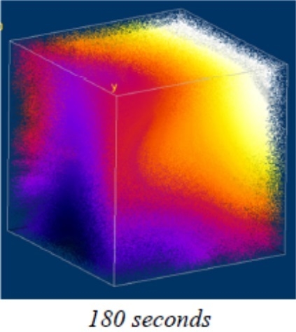
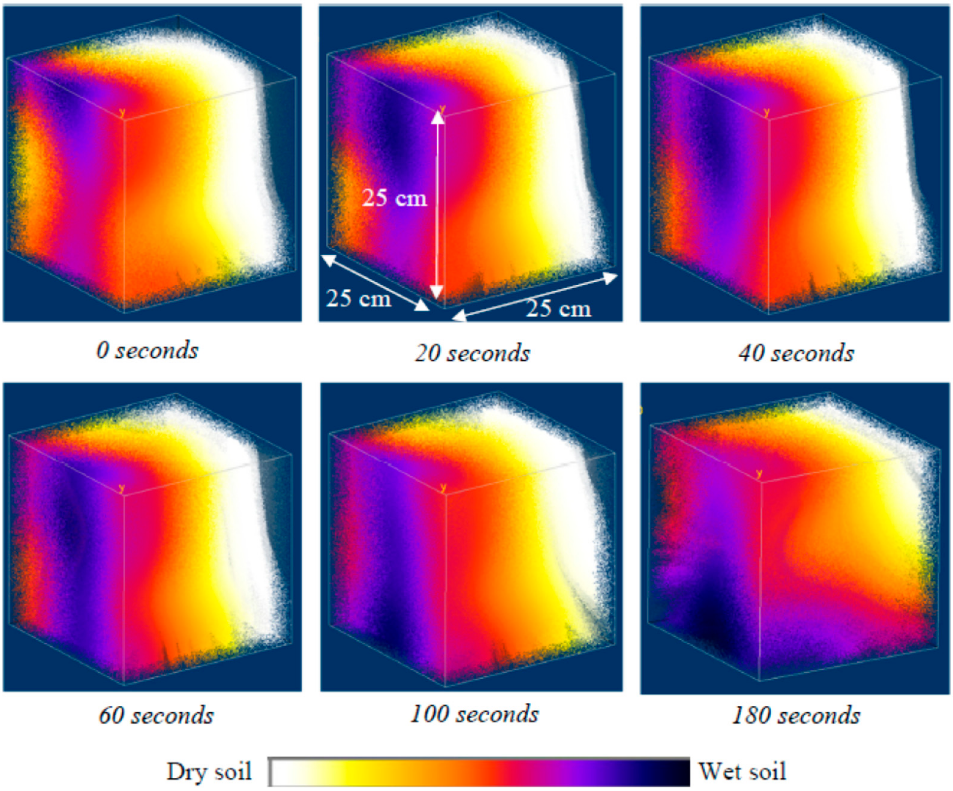
As opposed to many existing single-point sensors, the present system provides tomographical information on the three-dimensional distribution of relative moisture content in real time. The resistance values between various pairs of electrodes are measured multiple times per second and the present reconstruction algorithm can recover the approximated distribution at a similar rate. A more accurate inversion procedure may be developed in the future allowing for precise volumetric reconstruction. During its creation, the affordability of the present device was one of the main considerations for its wide use in the irrigation control and monitoring systems. With two calibration values (the resistance of dry soil and the resistance of properly irrigated soil), a user can decide when, where and how much water should be applied to the soil, as well as the time when irrigation should be stopped at a specific location. An example of three-dimensional soil moisture tomography of the described system is shown in Figure 12. The measured values are normalized by the moisture content of dry soil, which was measured before watering. This figure demonstrates how water penetration into soil can be tracked in real-time (as distinguished by the color in Figure 12, depicting a three-dimensional representation of dry soil regions where water was not applied yet as well as irrigated regions). The three-dimensional dynamics of water penetration can be observed with the help of the present system, as shown by the instantaneous snapshots in Figure 12. The present system can depict the relative moisture content between pre-calibrated dry and wet conditions, not the absolute value of the moisture content (which can be achieved by accurate single point devices). A real-time feedback for the irrigation control system can be implemented with the present instrument. If a multi-faucet irrigation system with independent controls is available, the described system can determine at what time the watering should be started and stopped at a specific location around plant roots, allowing minimal use of water and optimized efficiency of irrigation.
4. Conclusions
A standalone, affordable system that provides volumetric information on soil moisture distribution can be an attractive addition to the existing moisture sensors used in the irrigation control systems. Despite the fact that the present system requires frequent re-calibration and is inferior to many widely used moisture sensors in terms of absolute value of moisture concentration, it provides unique volumetric information on the relative moisture distribution within the sampled soil volume. Low-cost data acquisition devices can be sparsely distributed at various locations throughout an irrigated field and synchronized with real-time control systems. At the same time, historical data, which can be stored autonomously on each data acquisition device over a period of many months, can be used for future planning and optimization of watering procedures for each specific crop. Moreover, high efficiency of irrigation applied to the roots of specific plants can be achieved with this tomographic moisture information. The described system can be combined with environmental factors (e.g., temperature, humidity, wind, brightness of sun, etc.), which can be measured by the same device with the addition of various optional sensors. Although three-dimensional moisture measurements have been conducted previously [21,22,23], the ease of electrode installation and removal is an essential feature of the present device, making it attractive for multi-unit use in the agricultural field. By implementing the described system, farmers can significantly improve the efficiency of agricultural irrigation, leading to more food production with less water.
Acknowledgments
The author would like to thank his advisers, Betty Watson, Roxanna Jackman and Richard Tornai for their great advice, as well as the Contra Costa Economic Partnership (Walnut Creek, California) for their enthusiastic support of this project.
Conflicts of Interest
The authors declare no conflict of interest.
References
- Coping with Water Scarcity. UN—Water Thematic Initiatives. A Strategic Issue and Priority for System-Wide Action. 2006. Available online: http://www.unwater.org/publications/coping-water-scarcity/ (accessed on 5 September 2017).
- AghaKouchak, A.; Cheng, L.; Mazdiyasni, O.; Farahmand, A. Global warming and changes in risk of concurrent climate extremes: Insights from the 2014 California drought. Geophys. Res. Lett. 2014, 41, 8847–8852. [Google Scholar] [CrossRef]
- Hanak, E.; Mount, J.; Chappelle, C.; Lund, J.; Medellín-Azuara, J.; Moyle, P.; Public Policy Institute of California, Water Policy Center. What If California’s Drought Continues? Available online: http://www.ppic.org/publication/what-if-californias-drought-continues/ (accessed on 5 September 2017).
- Thompson, T.L.; Pang, H.C.; Li, Y.Y. The Potential Contribution of Subsurface Drip Irrigation to Water-Saving. Agric. Sci. China 2009, 8, 850–854. [Google Scholar]
- Bernstein, L.; Francois, L.E. Comparisons of drip, furrow, and sprinkler irrigation. Soil Sci. 1973, 115, 73–86. [Google Scholar] [CrossRef]
- Camp, C.R. Subsurface drip irrigation: A review. Trans. ASAE 1998, 41, 1353–1367. [Google Scholar] [CrossRef]
- Tagar, A.; Chandio, F.A.; Mari, I.A.; Wagan, B. Comparative Study of Drip and Furrow Irrigation Methods at Farmer’s Field in Umarkot. World Acad. Sci. Eng. Technol. 2012, 69, 863–867. [Google Scholar]
- Keeratiurai, P. Comparison of drip and sprinkler irrigation system for the cultivation plants vertically. J. Agric. Biol. Sci. 2013, 8, 740–744. [Google Scholar]
- Walker, J.P.; Willgoose, G.R.; Kalma, J.D. In Situ measurement of soil moisture: A comparison of techniques. J. Hydrol. 2004, 293, 85–99. [Google Scholar] [CrossRef]
- Susha Lekshmi, S.U.; Singh, D.N.; Baghini, M.S. A critical review of soil moisture measurement. Measurement 2014, 54, 92–105. [Google Scholar]
- Topp, G.C. Electromagnetic determination of soil water content: Measurements in coaxial transmission lines. Water Resour. Res. 1980, 16, 574–582. [Google Scholar] [CrossRef]
- Mojid, M.A.; Cho, H. Evaluation of the time-domain reflectometry (TDR)—Measured composite dielectric constant of root-mixed soils for estimating soil-water content and root density. J. Hydrol. 2004, 295, 263–275. [Google Scholar] [CrossRef]
- Rao, B.H.; Singh, D.N. Moisture Content Determination by TDR and Capacitance Techniques: A Comparative Study. Int. J. Earth Sci. Eng. 2011, 4, 132–137. [Google Scholar]
- Chanasyk, D.S.; Naeth, M.A. Field measurement of soil moisture using neutron probes. Can. J. Soil Sci. 1996, 76, 317–323. [Google Scholar] [CrossRef]
- Ozcep, F.; Yıldırım, E.; Tezel, O.; Asci, M.; Karabulut, S. Correlation between electrical resistivity and soil-water content based artificial intelligent techniques. Int. J. Phys. Sci. 2010, 5, 47–56. [Google Scholar]
- Afa, J.T.; Anaele, C.M. Seasonal Variation of Soil Resistivity and Soil Temperature in Bayelsa State. Am. J. Eng. Appl. Sci. 2010, 3, 704–709. [Google Scholar] [CrossRef]
- Abu-Hassanein, Z.S.; Benson, C.H.; Blotz, L.R. Electrical Resistivity of compacted clays. J. Geotech. Eng. 1996, 5, 397–406. [Google Scholar] [CrossRef]
- Bai, W.; Kong, L.; Guo, A. Effects of physical properties on electrical conductivity of compacted lateritic soil. J. Rock Mech. Geotech. Eng. 2013, 5, 406–411. [Google Scholar] [CrossRef]
- Samouëlian, A.; Cousin, I.; Tabbagh, A.; Bruand, A.; Richard, G. Electrical resistivity survey in soil science: A review. Soil Tillage Res. 2005, 83, 173–193. [Google Scholar] [CrossRef] [Green Version]
- Brunet, P.; Clément, R.; Bouvier, C. Monitoring soil water content and deficit using Electrical Resistivity Tomography (ERT)—A case study in the Cevennes area, France. J. Hydrol. 2010, 380, 146–153. [Google Scholar] [CrossRef]
- Tejero-Andrade, A.; Cifuentes, G.; Chávez, R.E.; López-González, A.E.; Delgado-Solórzano, C.L. CORNER-arrays for 3D electric resistivity tomography: An alternative for geophysical surveys in urban zones. Near Sur. Geophys. 2015, 13, 355–367. [Google Scholar] [CrossRef]
- Gravalos, I.; Moshou, D.; Loutridis, S.; Gialamas, T.; Kateris, D.; Bompolas, E.; Tsiropoulos, Z.; Xyradakis, P.; Fountas, S. 2D and 3D soil moisture imaging using a sensor-based platform moving inside a subsurface network of pipes. J. Hydrol. 2013, 499, 146–153. [Google Scholar] [CrossRef]
- Gravalos, I.; Georgiadis, A.; Kateris, D.; Haralampous, O.; Gialamas, T. 3D soil moisture sensing and imaging. In Precision Agriculture '15; Wageningen Academic Publishers: Gelderland, The Netherlands, 2015; pp. 17–26, eISBN: 978-90-8686-814-8; ISBN 978-90-8686-814-8. [Google Scholar]
- Gravalos, I.G.; Moshou, D.E.; Loutridis, S.J.; Gialamas, T.A.; Kateris, D.L.; Tsiropoulos, Z.T.; Xyradakis, P.I. Design of a pipeline sensor-based platform for soil water content monitoring. Biosyst. Eng. 2012, 113, 1–10. [Google Scholar] [CrossRef]
- Brillante, L.; Bois, B.; Lévêque, J.; Mathieu, O. Variations in soil-water use by grapevine according to plant water status and soil physical-chemical characteristics—A 3Dspatio-temporal analysis. Eur. J. Agron. 2016, 77, 122–135. [Google Scholar] [CrossRef]
- Herman, G.T. Fundamentals of Computerized Tomography: Image Reconstruction from Projection, 2nd ed.; Springer: New York, NY, USA, 2009. [Google Scholar]
- Malicki, M.A.; Hanks, R.J. Interfacial contribution to two-electrode soil moisture sensor readings. Irrig. Sci. 1989, 10, 41–54. [Google Scholar] [CrossRef]
- Geotomo Software Package for Geoelectrical IMAGING in 2D and 3D. Available online: http://www.geotomosoft.com/ (accessed on 17 November, 2017).
Figure 1.
(a) Schematic diagram of the solar-powered standalone data acquisition device. (b) One example of the electrode configuration. Such electrode arrays can be easily installed and removed in/out of soil.
Figure 1.
(a) Schematic diagram of the solar-powered standalone data acquisition device. (b) One example of the electrode configuration. Such electrode arrays can be easily installed and removed in/out of soil.

Figure 2.
(a) The principle of soil resistance measurement in the present system (shown for one pair of electrodes). (b) The principle of resistance measurements carried out by multiple electrode pairs.
Figure 2.
(a) The principle of soil resistance measurement in the present system (shown for one pair of electrodes). (b) The principle of resistance measurements carried out by multiple electrode pairs.
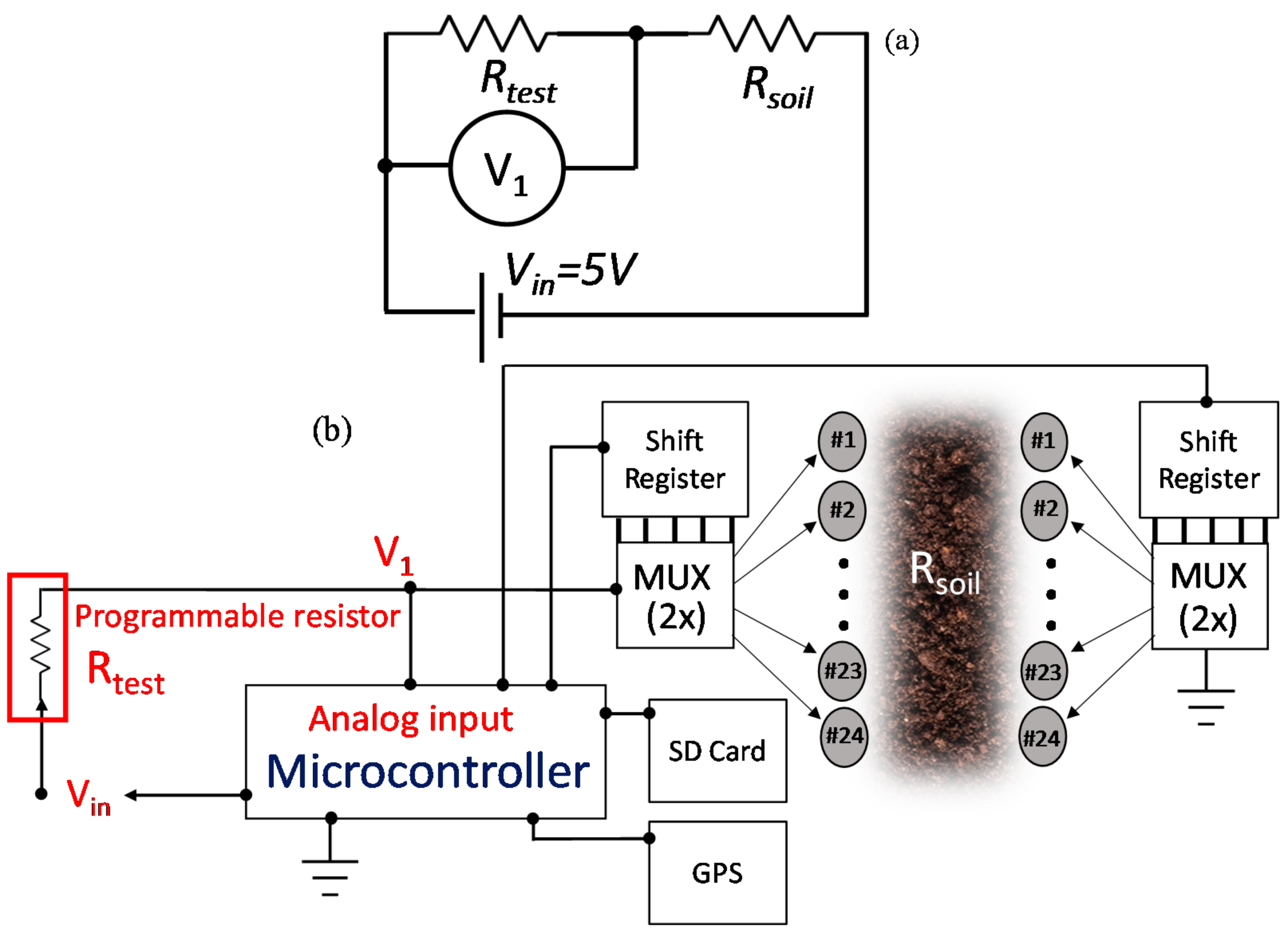
Figure 3.
Virtual lines representing current between electrodes on opposite arrays. Resistance measurements between all pairs of electrodes are used for volumetric reconstruction of soil moisture content.
Figure 3.
Virtual lines representing current between electrodes on opposite arrays. Resistance measurements between all pairs of electrodes are used for volumetric reconstruction of soil moisture content.

Figure 4.
Distribution of computer-simulated conduction current between two electrodes. (a) A 24 × 24 × 24 cm3 cube of dry soil (conductivity 0.002 S/m, density 1200 kg/m3) contains a 4 × 4 × 12 cm3 wet soil (conductivity 0.2 S/m, density 1400 kg/m3) volume. This volume representing wet soil is positioned between the two electrodes (b), farther away from the direct path between the electrodes (c) and the cube consisting only of a dry soil (d). This model demonstrates that the measured resistance depends on the location of the wet soil, despite the fact that the current flows through the entire soil volume.
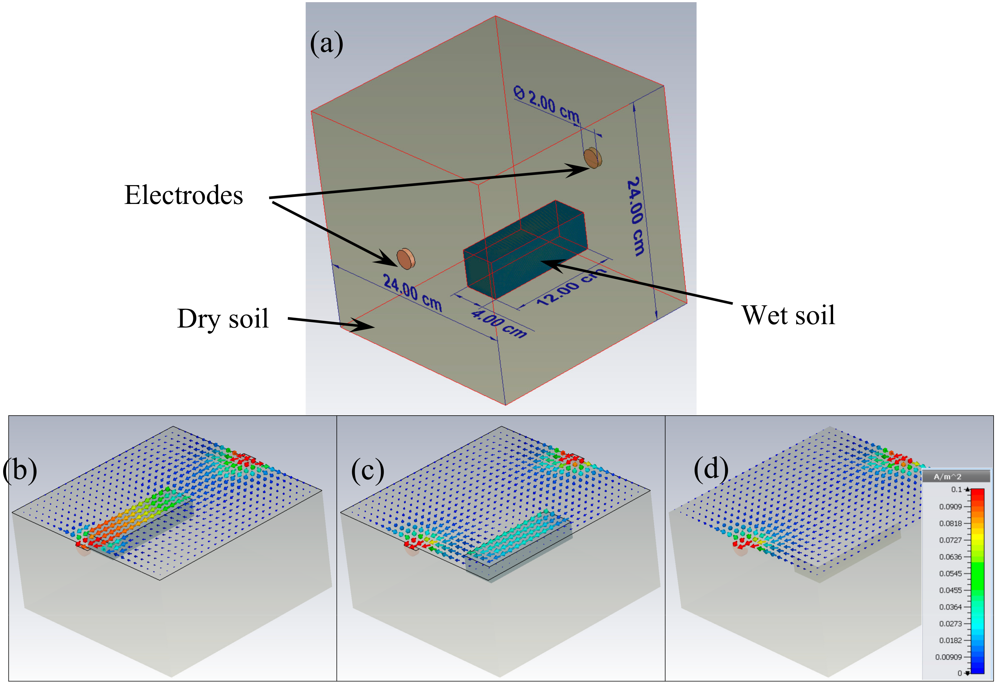
Figure 5.
The graph of soil resistance versus water content measured for two different soil types at 19 °C temperature. The logarithmic fit to the measured data is shown by two equations. Soil 1 initially contained more fertilizer, resulting in lower resistance values. Two electrodes with an area of 7.35 cm2 were placed 30 cm apart during this experiment.

Figure 6.
The graph of resistance versus the inverse area of electrodes measured for three different electrode separations.
Figure 6.
The graph of resistance versus the inverse area of electrodes measured for three different electrode separations.
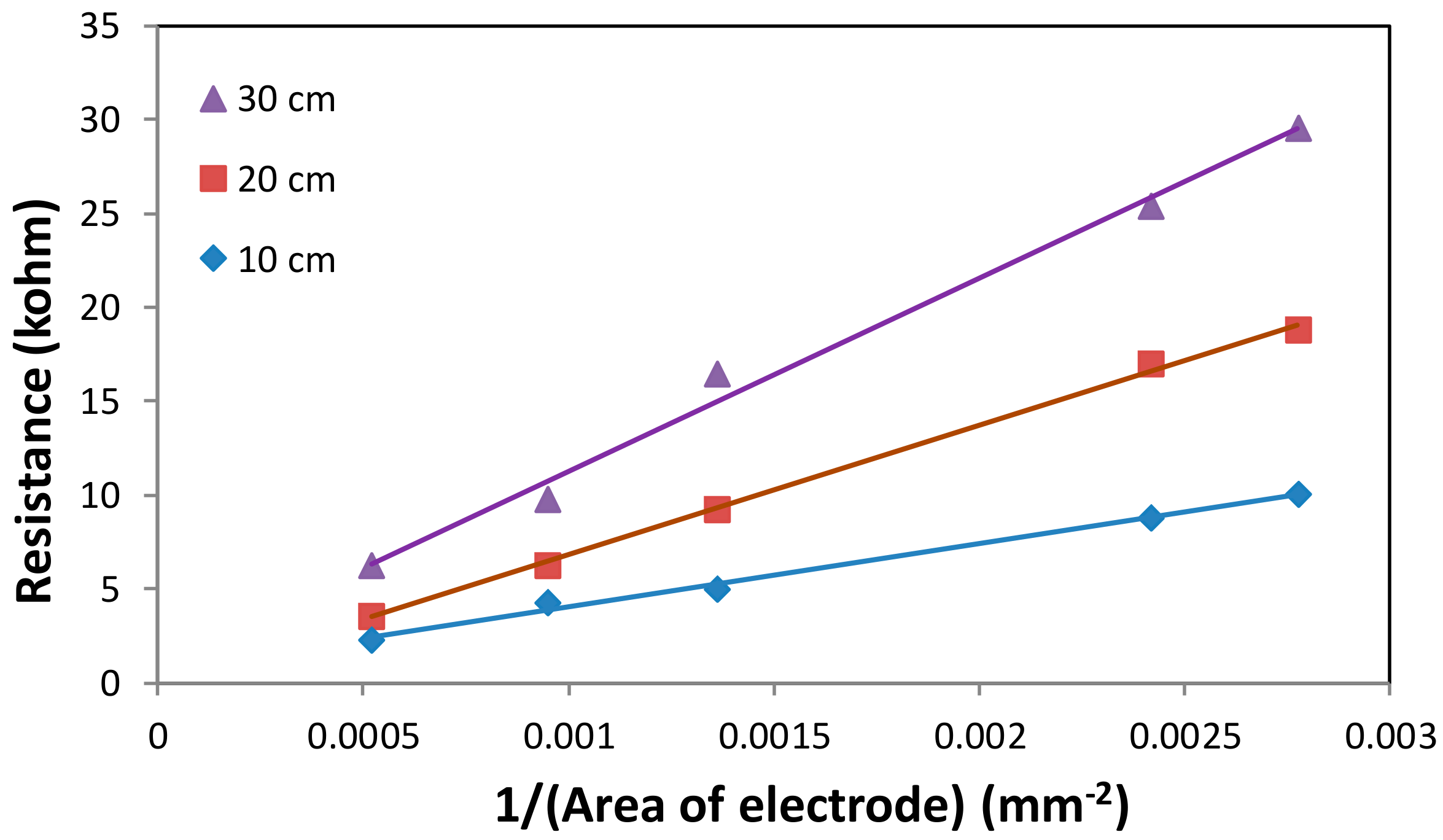
Figure 7.
Schematic diagram of the electrode configuration used in the measurements presented in Figure 8, Figure 9 and Figure 10. Water was applied predominantly in the area above electrode #13. A water barrier (container) was placed below the lowest row of electrodes (#1–#4) to demonstrate measurements of high moisture concentration.

Figure 8.
Relative resistance measured between pairs of electrodes shown as a function of time. At 7:29 water was applied to soil above electrode #13. Initially, the water accumulated near electrode #9 and did not seep through the soil for several minutes. This resulted in a rapid dip in resistance, shortly followed by a rapid increase.

Figure 9.
Relative resistance measured between pairs of electrodes at the bottom of the soil sample (electrode pairs #1–#4.), shown as a function of time. Water accumulated at the bottom of the soil sample, resulting in a rapid decrease of resistance for several electrode pairs.
Figure 9.
Relative resistance measured between pairs of electrodes at the bottom of the soil sample (electrode pairs #1–#4.), shown as a function of time. Water accumulated at the bottom of the soil sample, resulting in a rapid decrease of resistance for several electrode pairs.

Figure 10.
The relative resistance measured between electrode pairs #1, #5, #9, #13. While most of the water propagated to the bottom of the container, some accumulated near electrode #13, where it was initially applied and did not propagate downward for a relatively long time.
Figure 10.
The relative resistance measured between electrode pairs #1, #5, #9, #13. While most of the water propagated to the bottom of the container, some accumulated near electrode #13, where it was initially applied and did not propagate downward for a relatively long time.

Figure 11.
The average relative resistance values measured by all pairs of electrodes as a function of time. As soil dried, the measured resistance values gradually increased toward the values of a dry soil. The insert shows the recovery of soil resistance during drying over a period of several days, in between two consecutive applications of water.
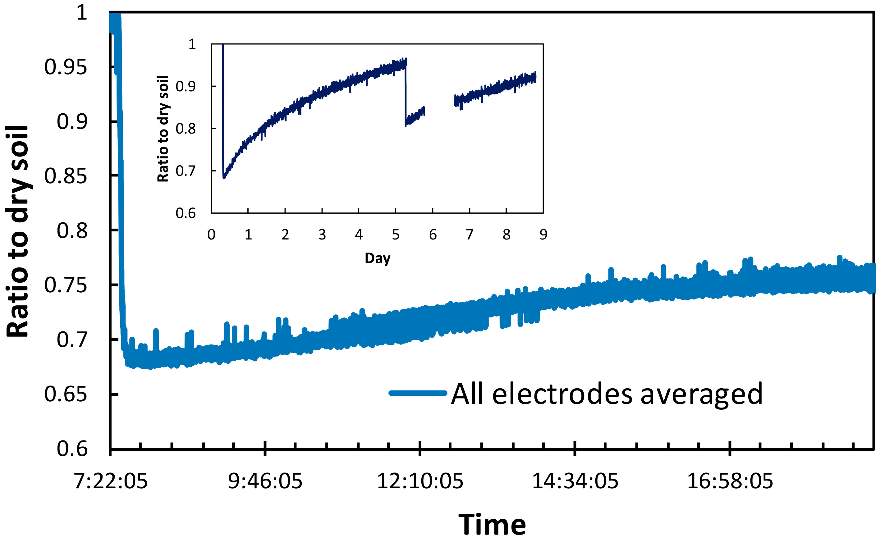
Figure 12.
Three-dimensional visualization of relative moisture content. Water was applied at the top left corner (as shown in Figure 7). Six consecutive images show the dynamics of water over ~3 min period. The time passed since water application is shown below each image.
Figure 12.
Three-dimensional visualization of relative moisture content. Water was applied at the top left corner (as shown in Figure 7). Six consecutive images show the dynamics of water over ~3 min period. The time passed since water application is shown below each image.

© 2017 by the author. Licensee MDPI, Basel, Switzerland. This article is an open access article distributed under the terms and conditions of the Creative Commons Attribution (CC BY) license (http://creativecommons.org/licenses/by/4.0/).
Share and Cite
MDPI and ACS Style
Tremsin, V.A. Real-Time Three-Dimensional Imaging of Soil Resistivity for Assessment of Moisture Distribution for Intelligent Irrigation. Hydrology 2017, 4, 54. https://doi.org/10.3390/hydrology4040054
AMA Style
Tremsin VA. Real-Time Three-Dimensional Imaging of Soil Resistivity for Assessment of Moisture Distribution for Intelligent Irrigation. Hydrology. 2017; 4(4):54. https://doi.org/10.3390/hydrology4040054
Chicago/Turabian StyleTremsin, Vasily A. 2017. "Real-Time Three-Dimensional Imaging of Soil Resistivity for Assessment of Moisture Distribution for Intelligent Irrigation" Hydrology 4, no. 4: 54. https://doi.org/10.3390/hydrology4040054
Note that from the first issue of 2016, this journal uses article numbers instead of page numbers. See further details here.