Development of Flood Warning System and Flood Inundation Mapping Using Field Survey and LiDAR Data for the Grand River near the City of Painesville, Ohio

Abstract

Flooding is one of the most frequent natural disasters across the world, which damages properties and may take the lives of people. Flood warning systems can play a significant role in minimizing those effects by helping to evacuate people from the probable affected areas during peak flash flood times. Therefore, a conceptual approach of an automated flood warning system is presented in this research to protect several houses, roads, and infrastructures along the Grand River, which are vulnerable to flooding during a 500 year return period flash flood. The Grand River is a tributary of Lake Erie, which lies in the Grand River watershed in the northeastern region of the United States and has a humid continental climate and receives lake-effect precipitation. The flood warning system for the Grand River was developed specifically during high flow conditions by calculating flood travel time and generating the inundation mapping for 12 different selected flood stages, which were approximately 2 to 500 years in recurrence interval, ranging from 10 ft. to 21 ft. at gage station 04212100, near the City of Painesville, OH. A Hydraulic Engineering Center-River Analysis System (HEC-RAS) was utilized for hydraulic modeling. Geospatial data required for HEC-RAS was obtained using a Digital Elevation Model (DEM) derived from Light Detection and Ranging (LiDAR) datasets, which were pre-processed and post-processed in HEC-GeoRAS to produce flood inundation maps. The flood travel time and flood inundation maps were generated by integrating LiDAR data with field verified survey results in order to provide the evacuation lead time needed for the people of probable affected areas, which is different from earlier studies. The generated inundation maps estimate the aerial extent of flooding along the Grand River corresponding to the various flood stages at the gage station near the City of Painesville and Harpersfield. The inundation maps were overlaid on digital orthographic maps to visualize its aerial extents, which can be uploaded online to provide a real-time inundation warning to the public when the flood occurs in the river.

1. Introduction

Flooding is a major natural hazard, which greatly impacts different regions across the world [1,2]. In the United States, floods take the lives of more people than any other form of natural disaster [3,4]. Among different types of floods, flash floods are the most dangerous, as these are the primary cause of deaths in the United States, killing more than 140 people each year [5]. A flash flood is an abrupt flow of a large amount of water in a river within a few minutes or hours due to intense rainfall, a dam or levee failure, or a sudden release of water held by an ice jam [5,6]. The Grand River is an example of a river that experiences flash floods frequently.

Several methods for hydrologic forecasts, ranging from simple index models to robust hydrological models, were developed in the past. Forecasts at various lead times, such as short term [7], medium range [8], and long range [9], could be either probabilistic or deterministic. One of the popularly used probabilistic forecasts, which is operational at the National Weather Service (NWS), a weather forecasting agency of the US Government for flood forecasting, is ensemble streamflow prediction [10].

Hydrologic forecasting is the approach typically used in NWS, USA for providing flooding information. For the prediction of flood inundation, surveyed river survey cross sections are typically needed for the development of hydraulic models [11].

Typically, elevation data such as National Elevation Datasets (NEDs) and Light Detection and Ranging (LiDAR) do not include the river bathymetry, leading to the requirement of field verification through topographical surveys. Flood warning systems developed using such data cannot make accurate predictions [11]. Therefore, high-resolution LiDAR and field verified survey data of bathymetry were integrated to develop a hydraulic model.

Flood warning systems help protect people’s lives and prevent property damages by providing sufficient lead time for evacuations [12]. For efficient flood management, two important factors should be taken into account, namely flood travel time and possible area of inundation. Flood travel time is key for the timely evacuation of people from probable flood prone areas. Our study has uniquely included the concept of calculating flood travel time using a hydraulic model. Likewise, flood inundation maps are also important tools that represent the spatial variability of flood hazards and provide a more clear picture and robust understanding of flood patterns [13,14], provided that they are carefully prepared and made easily accessible to the public [15].

There are some basic steps to be followed before and after flood occurrence for the development of an efficient flood warning system [16,17]. The steps before the flood occurrence are: generation of flood inundation maps for various flood stages, quantification of thresholds in maps, and identification of flood hazard areas for different flood scenarios. Similarly, the steps after the flood occurrence are: to inform concerned officials/authorities, issue warnings to the people of possible inundation areas, evacuate people from probable inundation areas, and conduct rescue operations.

The basic processes needed for the establishment of an effective flood warning system before the occurrence of a flood has been determined and described in this study. The primary objective of this research study was to calculate the flood travel time during a high flood period by developing a hydraulic model using the Hydraulic Engineering Center-River Analysis System (HEC-RAS) and to provide the model for the possible use by the NWS. All necessary digital files, including a rating curve to provide the evacuation times for the flood warning system for the Grand River, Ohio, were prepared. A series of flood inundation maps for 12 different selected high flood stages were generated using HEC-GeoRAS by combining field survey data with high resolution LiDAR data. The NWS has a legal responsibility for hydrologic forecasting throughout the nation [18,19]. The NWS Ohio River Forecast Center, located in Wilmington, Ohio, forecasts the peak stage flows based on the precipitation gages and streamflow gages in Ohio. Based on the river stages and the rating curve that we have reported in this study, the flood travel time and possible inundation area can be estimated from pre-developed flood inundation maps and flood warnings can be issued to the probable affected areas in the real time by uploading those pre-developed inundation maps online and providing access to the general public.

Similar approaches can be very useful for similar rivers during high flood conditions around the world in order to generate flood travel times and inundation maps for various return period floods. The use of calculated flood travel times can be helpful in planning for timely evacuations within short periods of time during flooding events. Inundation maps would be helpful for planners to focus on specific areas during evacuation actions. In general, this information leads to a more effective and efficient way of providing a warning system before the flood occurs and for the evacuation after the occurrence of flood events.

2. Theoretical Description

The hydraulic modeling software, HEC-RAS, was used in this study for steady and unsteady flow analysis. HEC-RAS was developed by the United States Army Corps of Engineers-Hydrologic Engineering Center (USACE-HEC), and has been widely used for steady flow analysis, unsteady flow simulation, movable boundary sediment transport computations, and water quality analysis [20]. Usually, a steady flow approach is used for floodplain management and flood insurance studies, whereas an unsteady flow approach is used for subcritical flow regimes, especially for dam break analysis and pressurized flow modules [20,21]. HEC-RAS solves one-dimensional Saint-Venant equations, using a four-point implicit method developed for natural channels [21] to simulate unsteady flow, which are derived from the continuity and momentum equations. This scheme is completely non-destructive, but marginally stable when it is run in a semi-implicit form which corresponds to a weighting factor θ of 0.5. The value of θ in HEC-RAS varies from 0.6 to 1, where the value of 1 provides the most stable form [21].

In steady flow simulation, HEC-RAS solves the energy equation to calculate water surface profiles from one cross section to another cross section with an iterative procedure called the standard step method [20].

Flood travel time is calculated based on the flood velocity during the peak flood time. During the peak flood time, a flood travels quickly in the channel section, as an area of flow is relatively less in a channel section than in a floodplain region. The equations to calculate channel velocity and travel time are given below.

$$V_{ch}=\frac{Q_{ch}}{A_{ch}}$$

(1)

$$T=\frac{X}{V_{ch}}$$

(2)

where V_ch is channel velocity in ft/sec; Q_ch is channel flow in cfs; A_ch is flow area in the channel; T is travel time in seconds that flood takes to travel from one cross section to the next; and X is the longitudinal distance between two corresponding cross sections.

3. Materials and Methodology

3.1. Study Area

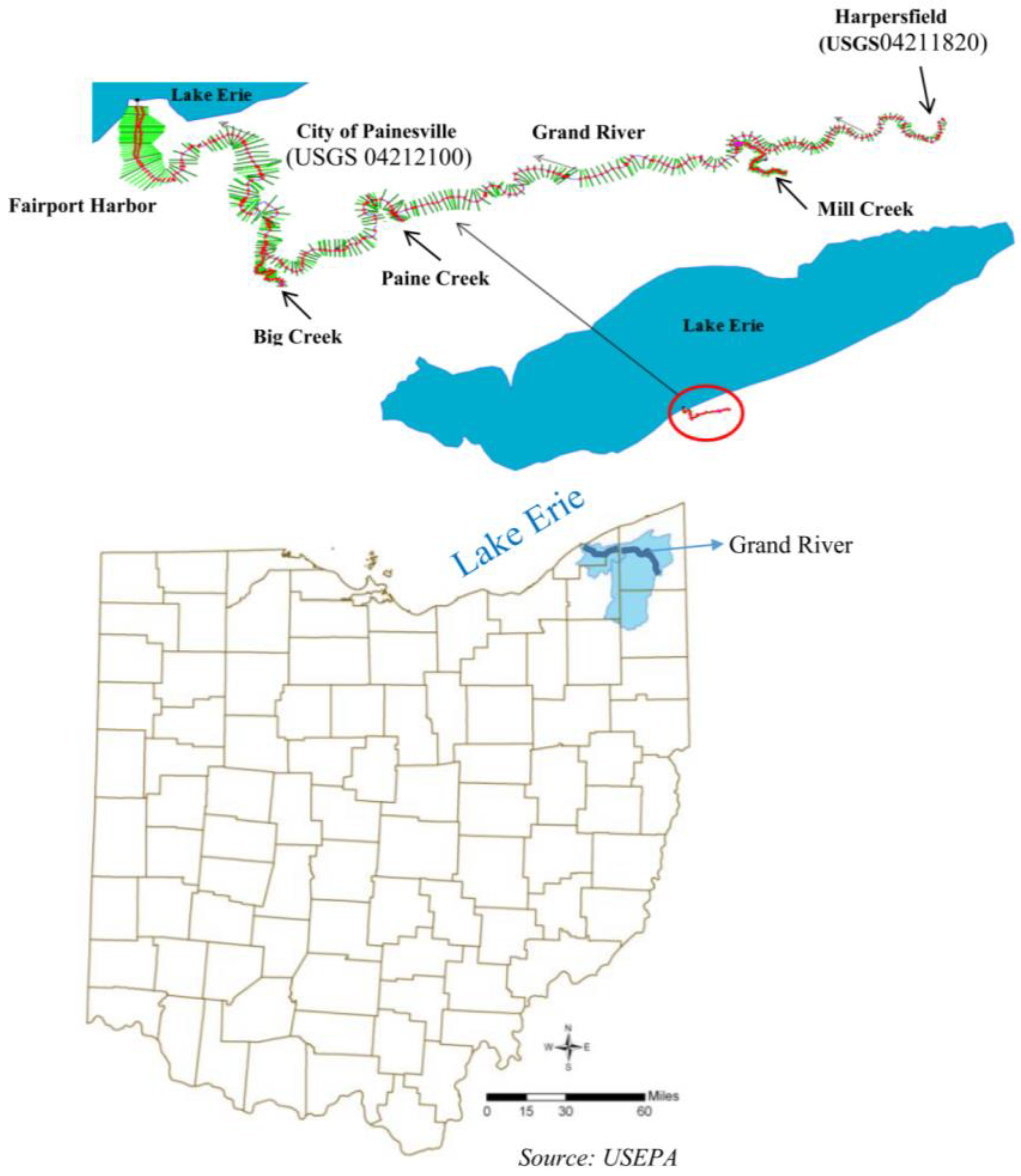
This study was conducted in the Grand River watershed, which is located in the Northeastern region of Ohio (Figure 1). The Grand River watershed has an area of 705 mi² which comprises of major three tributaries (Mill, Paine, and Big Creek) and an elevation range from minimum of 564 ft. to maximum of 1385 ft. above mean sea level. The river has an average slope of 1 in 900 with an average width of 275 ft. and a length of 102.7 miles which eventually meets Lake Erie to the North. 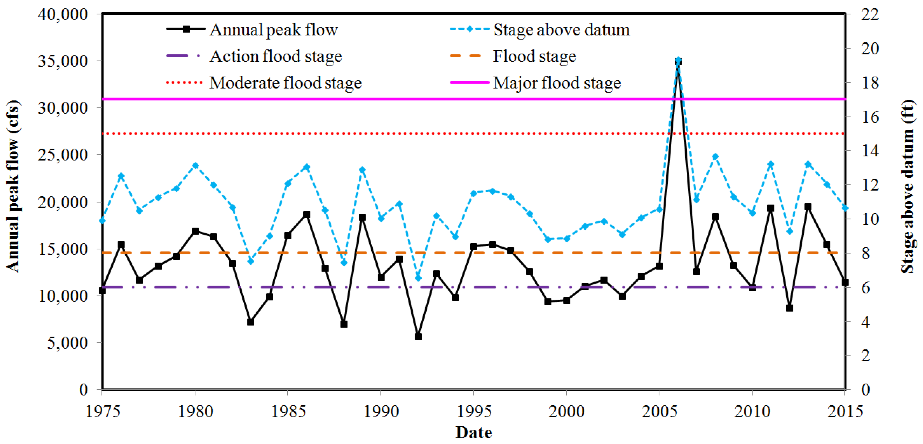However, more specifically, a portion of the Grand River starting from mouth of the river at Lake Erie to 32.2 miles up near Harpersfield (Figure 1) has been taken in consideration for the development of a hydraulic simulation. The watershed has a humid continental climate, therefore it experiences a large seasonal temperature variation with warm summers and freezing winters. Additionally, the watershed receives a large variation in precipitation because of the combination of lake influence and topographic features. The city of Painesville in Lake County, our area of interest, along the Grand River is one of the most affected regions due to the frequent flooding that has occurred from time to time (1989, 2006, 2008, and 2011). Extensive flooding of the Grand River was experienced on 27–28 July 2006 due to the intense rainfall of more than 11 inches depth that occurred in a short period of time; the flood resulted in property damages estimated at 30 million USD and one fatality in Lake County. Numerous people (600) had to be evacuated, and as a result, three counties (Lake, Geauga, and Ashtabula) were declared as Federal and State disaster areas [22]. The flood destroyed more than 800 homes and five bridges in Lake County. Additionally, it disrupted traffic by closing 13 roads near the city of Painesville. The peak discharge and stage for that event was estimated to be 35,000 cfs and 19.35 ft., respectively (Figure 2), as recorded by United States Geological Survey (USGS) gauge station (04212100) near the city of Painesville.

3.2. HEC-GeoRAS/HEC-RAS Model Input

Since our analysis (not shown in this manuscript) indicates that a HEC-RAS model developed through the combined use of field survey results and LiDAR would make better predictions, we utilized survey data in combination with LiDAR data [23]. Elevation data from surveys of the channel sections tend to be more representational of the channel sections, as LiDAR cannot penetrate the water bodies, whereas LiDAR provides good elevation information for the surrounding flood plain [23]. Since it is not practical or economically feasible to survey each and every section of the river, especially in flood plain zone, we conducted a detailed survey in 77 cross sections of the river at approximately every half a mile or so. The LiDAR data were utilized for the rest of the flood plain section. The unsteady HEC-RAS model was calibrated by the iterative process to obtain a suitable value of Manning’s roughness for river reaches by comparing simulated stage and discharge with the observed data. Eight different flood events from 1996 to 1998 were used in the HEC-RAS simulation.

3.3. Overall Flood Warning Approach

An approach for a better flood warning system was developed in this study using field survey and high-resolution LiDAR data. The river was surveyed using a highly accurate Global Positioning System (GPS) Rover that uses the state Virtual Reference Station (VRS) System and allows Real Time Kinematic (RTK) positioning using a single rover in the field with no need to set up a base station. For bathymetry data near to the Fairport harbor, we obtained the pre-existing surveying data obtained by sounding method which was developed by the National Oceanic and Atmospheric Administration (NOAA) and USACE. A similar approach has been used to develop the flood warning systems of other areas in Ohio, such as in Findlay County [18] and Licking County [19]. Our approach was different from the earlier studies, as we utilized high-resolution datasets in the flood plain along with the field survey data in order to improve predictive accuracy and to better plan for the evacuation of people from probable flood prone areas. The warning system includes the consideration of travel time, which can be used to help plan for the evacuation of people from the possible flood inundation areas. The following steps have been followed in the process of developing a fully operational flood warning system.

3.3.1. Development of a Hydraulic Model

A fully functional HEC-RAS model was developed for this study. The calibrated/validated unsteady HEC-RAS model was used to run the hydraulic simulation. The unsteady HEC-RAS model was calibrated through an iterative process to obtain a realistic value for Manning’s roughness, which was accomplished by comparing observed stage/discharge with the simulated stage/discharge. Various statistical parameters such as Nash-Sutcliffe efficiency (NSE), R-squared (R²), percent bias (PBIAS), and root mean square error (RMSE) were used to test the accuracy and predictive power of the hydraulic model [24,25,26]. The model was further calibrated for steady flow scenario using high-water mark profiles of the 2006 flood event (

Table 1. Comparison of high-water mark profile and modeled profile for 2006 flood.

S.N	Community (Location)	State Plane Coordinate System		High-Water Mark Elevation (ft.)	Simulated Water Surface Elevation (ft.)	Error (ft.)
		Latitude	Longitude
1	Leroy Township	2,328,226.99	752,438.17	640.52	640.14	−0.38
2	Painesville Township	2,315,214.36	745,057.64	622.12	621.31	−0.81
3	City of Painesville	2,315,591.23	750,428.41	616.38	616.57	0.19
4	City of Painesville	2,315,665.58	750,530.73	614.49	615.00	0.51
5	City of Painesville	2,312,665.85	753,422.90	605.92	605.13	−0.79
6	City of Painesville	2,312,506.90	753,926.77	602.84	603.80	0.96
7	Painesville Township	2,314,266.22	758,102.79	596.14	594.97	−1.17
8	Painesville Township	2,313,812.87	757,994.98	595.66	595.70	0.04
9	City of Painesville	2,306,518.39	759,105.05	585.98	584.67	−1.31
10	City of Painesville	2,305,348.55	756,051.50	582.82	582.44	−0.38
11	City of Painesville	2,313,981.20	751,619.78	609.09	609.07	−0.02
12	City of Painesville	2,313,517.46	752,220.45	606.70	606.91	0.21
13	City of Painesville	2,313,886.29	752,934.42	605.79	605.13	−0.66
14	Painesville Township	2,314,792.43	758,414.14	595.25	594.19	−1.06
15	Painesville Township	2,308,230.02	761,356.54	589.25	587.89	−1.36
16	Village of Fairport Harbor	2,306,000.70	758,186.61	585.64	584.36	−1.28
17	Village of Fairport Harbor	2,304,355.87	756,543.63	581.64	581.19	−0.45
18	Village of Fairport Harbor	2,305,118.25	756,250.70	580.93	582.21	1.28
19	Village of Fairport Harbor	2,303,675.01	756,432.80	578.75	580.50	1.75

). Typically, a steady HEC-RAS model is calibrated using high-water mark profiles obtained from the survey during a flood event [27]. In this study, the high-water mark elevation points were compared with the modeled water surface elevation points to evaluate the model’s efficiency. The USGS conducted a survey to obtain high-water mark profiles along the Grand River using standard surveying technique during the 2006 flood, and those high-water mark elevation points were collected for use in this study from Ebner et al. (2007). However, it should be noted that the surveyed data of high-water marks may not always be accurate, as debris and sediments may not be available during the time of the high flood conditions [22].

This hydraulic model will be shared with NWS so that they can utilize the model in order to simulate and generate inundation maps for other various flow scenarios.

3.3.2. Development of Rating Curve

The rating curve was developed for high flow periods for the stream gage 04212100 near the city of Painesville. The developed rating curve was utilized to predict the flood discharge for 12 different selected floods (based on the flood stage of 10 ft. to 21 ft. at downstream gage station 04212100, as shown in

Table 2. Discharge values for various selected stages at 04212100 based on developed rating curve.

Stage at USGS Gage Stations				Discharge (cfs)
04211820 (Datum Level-733 ft.)		04212100 (Datum Level-595.59 ft.)		Painesville (04212100)	Harpersfield (04211820)		Big Creek	Paine Creek	Mill Creek
Stage in ft. Above Datum	Elevation (ft.) in NAVD 88	Stage in ft. Above Datum	Elevation (ft.) in NAVD 88	Drainage Area
				685 mi2	552 mi2	35.7 mi2		27.3 mi2	19.3 mi2
10.13	743.13	10.00	605.59	10,451.82	8422.49	544.72		416.55	294.48
11.07	744.07	11.00	606.59	12,404.48	9996.02	646.48		494.37	349.50
11.99	744.99	12.00	607.59	14,504.02	11,687.91	755.90		578.04	408.65
12.86	745.86	13.00	608.59	16,747.87	13,496.09	872.85		667.47	471.87
13.68	746.68	14.00	609.59	19,133.68	15,418.68	997.19		762.55	539.10
14.53	747.53	15.00	610.59	21,659.35	17,453.96	1128.82		863.21	610.26
15.35	748.35	16.00	611.59	24,322.93	19,600.38	1267.63		969.37	685.30
16.15	749.15	17.00	612.59	27,122.62	21,856.48	1413.54		1080.95	764.18
16.96	749.96	18.00	613.59	30,056.76	24,220.92	1566.46		1197.88	846.85
18.10	751.10	19.35	614.94	34,228.37	27,582.57	1783.87		1364.14	964.39
18.62	751.62	20.00	615.59	36,322.26	29,269.91	1893.00		1447.59	1023.39
19.42	752.42	21.00	616.59	39,650.82	31,952.19	2066.47		1580.24	1117.17

) in the Grand River to be used in the hydraulic model. The rating curve equation was developed using the daily discharge data greater than the 75th percentile for the period of 1988–2005. Since the practical purpose of developing the rating curve in this study was to estimate the streamflow during high flood time, the rating curve was developed using the 75th percentile flow in order to capture all high flood discharge values. It is noteworthy to mention that the rating curve developed for higher flow conditions may not be applicable during low flow conditions and vice versa. Since our interest is for high flood conditions, the warning system developed using this rating curve might not work for low flood conditions. A new rating curve has to be generated for low flood periods if a warning system is to be developed during low flood periods.

3.3.3. Preparation of Digital Flood Inundation Maps

The digital flood inundation maps for 12 different selected flood stages were generated using HEC-GeoRAS software (v10.1, Davis, CA, USA) based on the steady flow simulation performed in HEC-RAS. The digital flood inundation maps were generated based on the upstream and downstream gage height. These digital maps could be uploaded online in the National Portal System or Regional Portal System to provide the real-time flood inundation information to the public.

3.3.4. Installation of Siren System

For an effective flood warning approach, a siren system should be installed at various suitable locations near the city of Painesville to warn the people before the flood affects the probable impact areas along the Grand River.

3.3.5. Evacuation Time

The flood travel time for 12 different selected flood scenarios was calculated based on the hydraulic simulation in HEC-RAS which can be used for the evacuation of people using the warning system that has travel time included for probable inundation areas. This will provide valuable information to the public regarding evacuation time and probable inundation areas for several flood stages. Hence, this information can be used to relocate people to safer places within sufficient lead time. However, in order to develop a fully automated flood warning system, stream gages with automated equipment need to be installed in various places, which will be discussed later in the recommendation section.

4. Results and Discussion

4.1. Unsteady Flow Scenario

The historical annual peak flow/stage and various flood stage levels in the Grand River, Ohio, as per NWS [28], is shown in Figure 2. The unsteady model was calibrated and validated for both stage and discharge. The performance of the model showed good calibration and validation for the time period of 1996–1998, which was evaluated using statistical parameters and visual inspection method.

The hydraulic model was evaluated using different statistical measures, as mentioned above, and the model performance during calibration and validation for stage and discharge have been reported. The performance of the model showed good calibration and validation based on the evaluation measured through different statistical criteria. The calculated value of all statistical parameters was higher than the recommended values (NSE > 0.50, PBIAS ±25%, and RSR ≤ 0.70) [26]. The detailed results of calibration/validation for the stage at upstream gage station 04211820 are presented in

Table 3. Calibration/validation for stage at upstream gage station 04211820. NSE, Nash-Sutcliffe efficiency; PBIAS, percent bias; RMSE, root mean square error.

S.N	Date		Statistical Parameter
	From	To	NSE	R2	PBIAS	RSR	RMSE (ft.)
Calibration
1	3/1/1996 0:00	3/30/1996 0:00	0.74	1.00	0.05	0.51	0.53
2	4/15/1996 0:00	5/12/1996 23:00	0.84	1.00	0.00	0.39	0.60
3	10/20/1996 0:00	11/28/1996 23:00	0.84	1.00	0.03	0.40	0.58
4	2/4/1997 0:00	2/10/1997 23:30	0.83	1.00	0.02	0.41	0.53
Validation
5	2/26/1997 0:00	3/3/1997 23:30	0.81	1.00	−0.07	0.43	0.89
6	3/5/1997 0:00	3/19/1997 23:30	0.82	1.00	0.00	0.43	0.37
7	5/15/1997 0:00	6/6/1997 23:00	0.85	0.99	0.02	0.39	0.98
8	4/10/1998 0:00	4/30/1998 0:00	0.89	1.00	0.02	0.33	0.50

. Similarly, the detailed results of calibration/validation for discharge at downstream gage station 04212100 are presented in

Table 4. Calibration/validation for discharge at downstream gage station 04212100.

S.N	Date		Statistical Parameter
	From	To	NSE	R2	PBIAS	RSR	RMSE (cfs)
Calibration
1	3/1/1996 0:00	3/30/1996 0:00	0.74	0.88	11.04	0.51	589.73
2	4/15/1996 0:00	5/12/1996 23:00	0.72	0.86	9.18	0.53	1254.49
3	10/20/1996 0:00	11/28/1996 23:00	0.90	0.96	8.85	0.31	612.91
4	2/4/1997 0:00	2/10/1997 23:30	0.84	0.92	1.26	0.40	614.34
Validation
5	2/26/1997 0:00	3/3/1997 23:30	0.33	0.70	5.20	0.82	2683.32
6	3/5/1997 0:00	3/19/1997 23:30	0.69	0.85	7.37	0.56	723.70
7	5/15/1997 0:00	6/6/1997 23:00	0.80	0.92	−3.34	0.45	1722.91
8	4/10/1998 0:00	4/30/1998 0:00	0.83	0.92	3.24	0.41	784.87

. In this study, NSE for stage calibration/validation varied from 0.74 to 0.89 (Table 3), and NSE for discharge calibration/validation varied from 0.69 to 0.96 (Table 4) except for the period from 26 February 1997 to 3 March 1997.

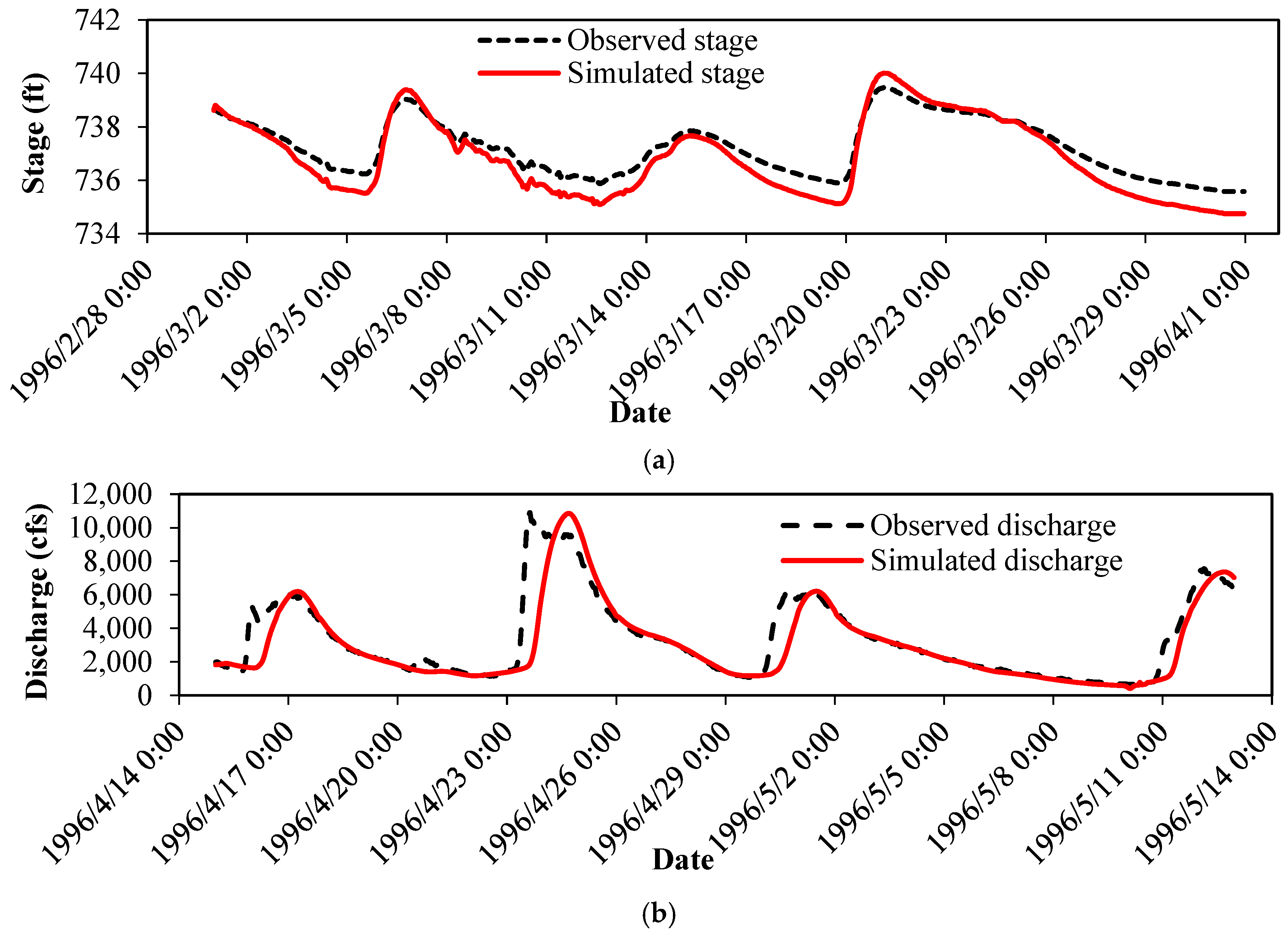
Furthermore, the performance of the model was also evaluated through visual inspection using the graphical plot of observed and simulated stage/discharge (Figure 3a,b). The calibration/validation of stage was conducted at upstream gage station 04211820, and the calibration/validation of discharge was conducted at downstream gage station 04212100. The model efficiency was assessed for several possible values of Manning’s roughness, and the roughness value was calibrated based on the performance efficiency of simulated result with observed data. The dynamic model calibration and validation was also performed in order to see the difference in the results of statistical parameters. For this, different Manning’s roughness values (0.020 to 0.035) were assigned to the river channel sections depending upon the channel characteristics. This did not result in the improvement of the model performance in stage calibration/validation. Also, dynamic calibration did not significantly change the performance of the model in terms of discharge calibration/validation. Hence, dynamic calibration/validation is assumed to have no significant impacts in a comparative study of floodplain maps and the travel time as long as the model is calibrated and validated with a value of Manning’s roughness that is able to adequately characterize the channel and floodplain characteristics. Hence, overall, the model performance for Manning’s roughness values in flood plains and river channels was well above the satisfactory range, and a value of 0.035 was adopted for channels and 0.15 was adopted for banks/floodplain regions.

4.2. Steady Flow Scenario

The steady flow model was calibrated to match the high-water mark profiles of the 2006 flood event. The drainage area ratio method was used to estimate the discharge of the remaining three tributaries because of unavailability of gage readings. The streamflow data for all rivers that were taken into consideration are shown in Table 2. The high-water mark profiles were compared with simulated water surface elevation for the 2006 flood in the Grand River in 19 locations, with the information presented in Table 1. The errors associated with water surface elevation ranged from 0.02 ft. to 1.75 ft. The errors were less than 1 ft. in 12 different locations and within 1.36 ft. for most of the locations.

4.3. Rating Curve

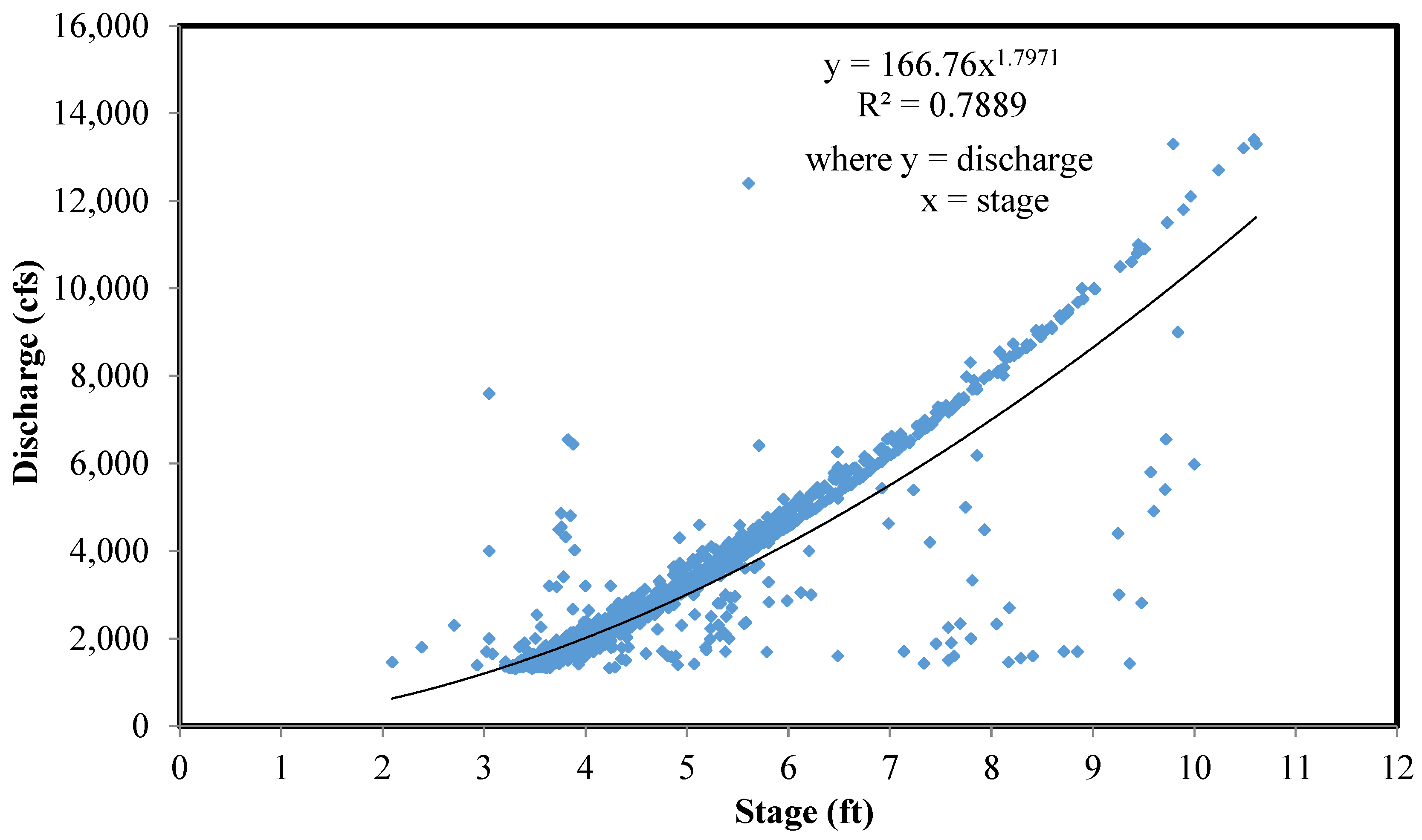
The rating curve for the stream gage near the city of Painesville was developed using 75 percentile exceedance discharge values for the period of 1988–2005 in order to capture all the high flood discharge values (Figure 4). The equation used for developing the rating curve is given below.

$$Q=166.67 H^{1.7971}$$

(3)

where Q is flow discharge (cfs) and H is the stage (ft.) of water in the river.

The developed rating curve was validated from the period of January 2006 to January 2015 with a NSE of 0.91 (Figure 5). However, the rating curve developed using entire datasets under-predicted the high flow, especially during flood period. This is not surprising, as the stage-discharge relationship (rating curve) varies depending upon the flood stage; therefore, the rating curve developed for a low flood stage may not necessarily be true for a higher flood stage. As stated earlier, modification of the rating curve equation will be necessary while generating for low flood conditions in the river.

4.4. Calculation of Travel Time and Development of Profiles/Flood-Inundation Maps

The simulation was performed in steady state condition to generate the profile for 12 stages from 10 ft. to 21 ft. with 1 ft. increments at the Grand River near the city of Painesville. However, 19.35 ft. was selected instead of 19.00 ft. in order to represent the flood of July 2006, which approximately corresponds to a 500 year return period flood. Discharge values corresponding to the selected stages were calculated using the rating curve developed at station 04212100. As there were not any recorded flows for the tributaries of the Grand River, including Mill, Paine, and Big Creek, discharges for various selected stages for those tributaries were estimated using a simple drainage area ratio. The estimated streamflow data for selected stages are presented in Table 2. The water surface extents modeled in HEC-RAS were then transferred to HEC-GeoRAS for the development of flood inundation maps for those selected stages. The flood inundation maps were then superimposed onto digital imagery maps produced by the Ohio Geographically Referenced Information Program (OGRIP) to see the aerial extents of flooding. The generated inundation maps for 12 different selected stages are presented in Supplementary Materials of this chapter.

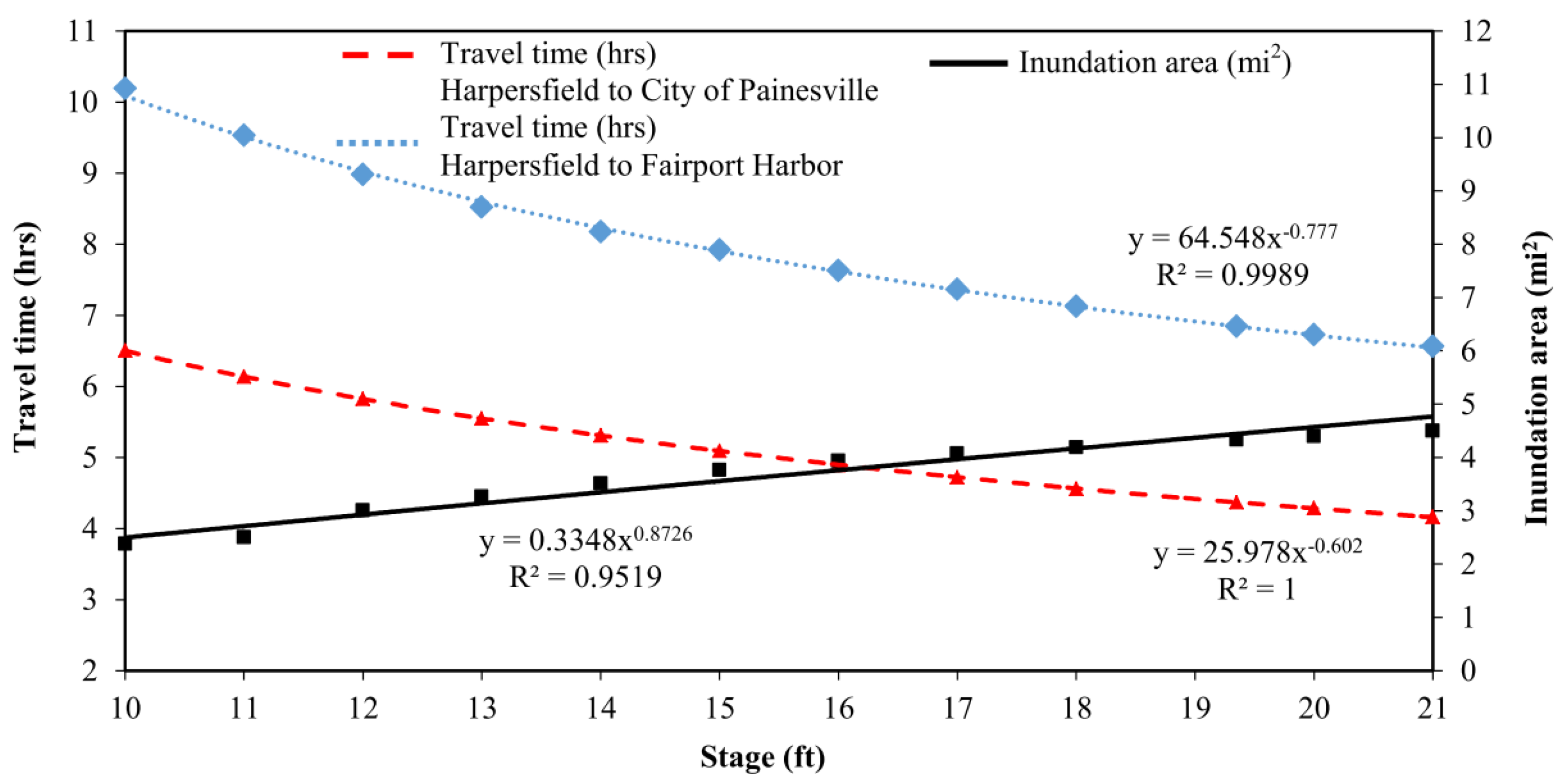
Flood travel times to reach the city of Painesville and Fairport Harbor, including the flood inundation areas, were calculated for various flood stages at gage station 04212100, near the city of Painesville (Figure 5). The equations for calculated travel time and predicted inundation area were also developed so that they could be used to estimate travel time and inundation area for other flood stages (Figure 6). The information regarding travel time and inundation areas can be utilized to evacuate people from the probable affected areas during various return period floods, which also helps for planning and decision making phase during flood events.

4.5. Flood Damages along the Grand River

Many houses, apartments, roads, bridges, and parks along the Grand River are more susceptible to flooding due to a 500 year return period flood as shown in the study area. The flood inundation map corresponding to a 500 year return period flood is shown in Figures in the Supplementary Materials (Figures S1–S12). Since this study was particularly focused in the city of Painesville, some houses, bridges, and parks along the Grand River which are beyond the study area and which may be susceptible to flooding might have been excluded here. Detailed information can be obtained from the flood map attached in the Supplementary Materials for the 19.35 ft. stage at gage station 04212100. The major affected areas according to the hydraulic simulation are Hidden-Valley Park near South Madison Road, Helen Hazen Wyman Park near the junction of Grand River, and Big Creek, Mill Stone Drive, Steel Avenue, and Grand River Avenue near Main Street, Kiwanis Recreation Park, Huntington Road near Lakeland Freeway, and the treatment plant and park near St. Clair St. bridge in the city of Painesville area. Similarly, other highly probable affected areas in Fairport are Western Reserve Yacht Club, Ram Island, Hidden Harbor Drive area, and Fairport Harbor Yacht Club. There are more than 30 houses near Grand River Avenue and Steel Avenue which are susceptible to flooding. Almost all the areas of Kiwanis Recreation Park including more than five houses on Huntington Road could be expected to be inundated. Also, there are approximately 20 houses susceptible to flooding along the Big Creek and at the junction of Big Creek and Grand River. Moreover, there are approximately 35 houses near Hidden Harbor and Fairport Road in Fairport that are highly vulnerable to flooding. Based on our analysis, almost all the harbors along the Grand River in Fairport might be affected by the flood. Therefore, when the stage at gage station 04212100 near the city of Painesville exceeds 19.35 ft., the situation might be worse compared to what was experienced in the 2006 flood. The damages due to floods of various stages along the Grand River can be obtained from the 12 different flood maps attached in the Supplementary Materials.

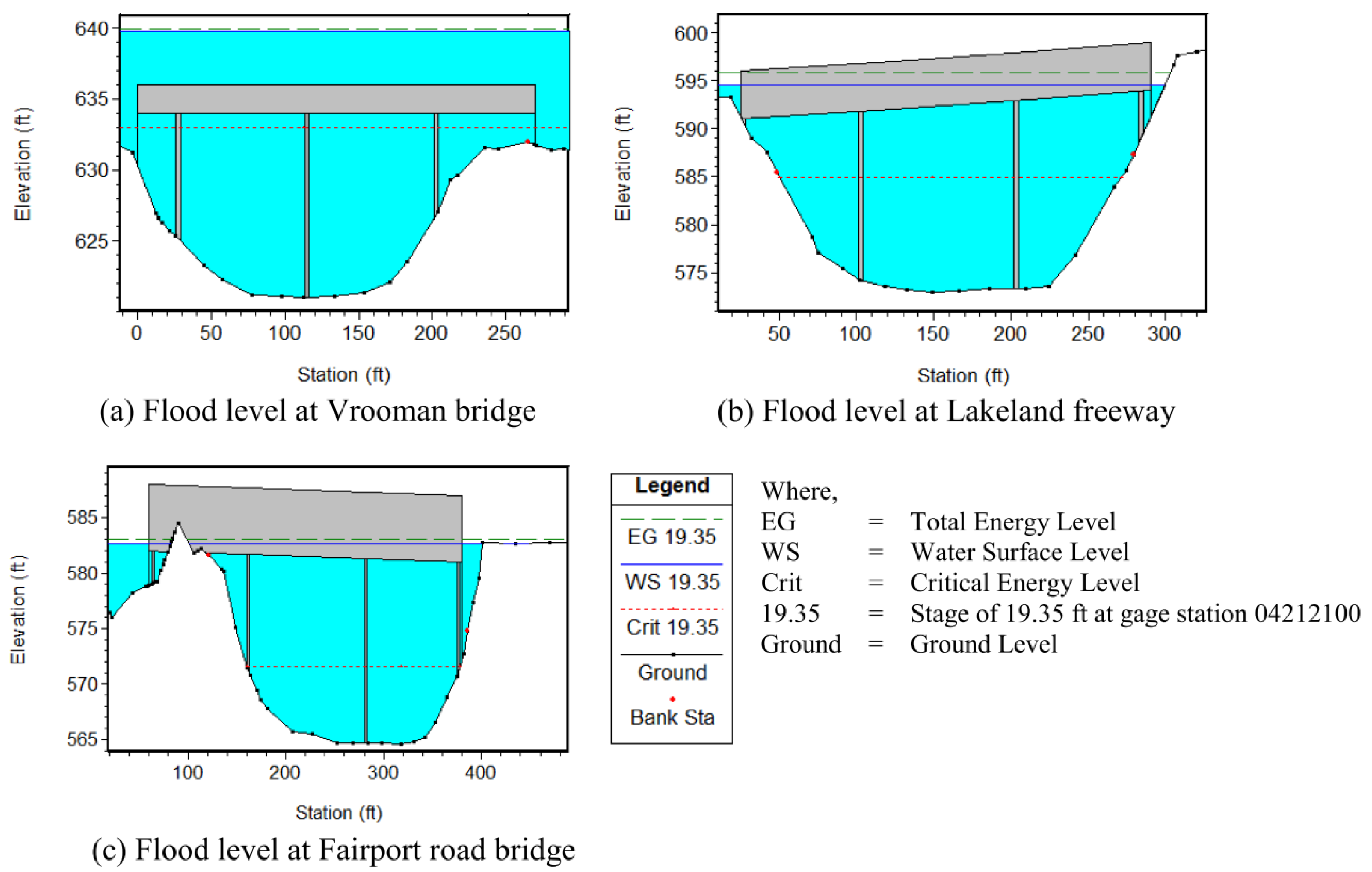
Likewise, the potential susceptibility of bridges and roads in Painesville and Fairport to flood conditions was determined. Flood levels for different bridges that might be affected by 500 year return period floods are shown in Figure 6. Bridges at Vrooman road, Lakeland freeway, and Fairport road have a high likelihood of flooding during a 500 year return period flood. Among those bridges, Vrooman Bridge was found to be more likely to be critically impacted, as water levels were projected to significantly rise (>3 ft.) above the road level (Figure 7a). Similarly, the flood levels for the other two bridges are shown in Figure 7b,c. Given this information, alternative routes for the aforementioned potentially affected bridges and roadways should be established.

In addition, flash floods have a higher likelihood of carrying large amounts of debris and sediments [29]. The effects of debris and sediment in increased flood level and floodplain mapping have not been considered in this study. Large woody debris has the capability to affect the hydraulics and hydrology of channel and floodplain areas [30], potentially causing a rise in water level at bridges, weirs, and other control structures [29]. As such, the potential sites where a debris jam could occur should be studied in order to accurately simulate flood inundation maps.

5. Conclusions

Flood warning systems should be developed carefully and precisely in order to help reduce the negative consequences of a flood hazard. There is an increasing need to develop reliable flood warning systems in order to reduce the greater risks associated with flooding. In this study, an approach to developing a flood warning system was described for the Grand River by estimating flood travel time and flood inundation boundaries for 12 selected flood stages at gage station 04212100 near the city of Painesville. HEC-GeoRAS was used for pre-processing to prepare geospatial data required for hydraulic analysis and a one dimensional hydraulic model, HEC-RAS, was used to perform hydraulic analyses for different flood stages. The unsteady flow model was developed to calibrate the Manning’s roughness value. This unsteady flow model can be utilized in the future for flood prediction in this region.

A rating curve for high flood periods was developed using the historical stage/discharge data and was utilized to estimate the peak flood discharge for different flood stages. Due to a lack of gaged discharge/stage datasets, a simple drainage area ratio method was used to calculate the peak flow for corresponding flood stages for three small tributaries within the study area. Flows from other ungagged minor creeks present in the drainage area were not considered in the model. The post-processing was performed again in HEC-GeoRAS to generate flood inundation maps for 12 different selected flood stages that ranged from approximately 2 to 500 year recurrence periods. The generated inundation maps were overlaid with digital orthographic maps to see aerial extents of various floods. The generated flood inundation maps for 12 different flood stages could be refined and further calibrated considering all sources of streamflow in the model. Furthermore, reestablishing the discontinued stream gage in Harpersfield and installing new stream gages for each of the tributaries (e.g., Mill, Paine, and Big Creek) would help with the collection of real time series data, which could then be fitted to an unsteady flow model to generate more accurate flood inundation maps.

Finally, it is expected that the rating curve, digital files, and/or flood inundation maps can be utilized to issue flood warnings in this region. In addition, the analysis will be useful to NWS, decision makers, and emergency flood management agencies for the preparation and management of the situation before and after flooding events along the Grand River, near the city of Painesville. As a conclusion of this study, the concepts that have been used in this study can be applied to other rivers with similar characteristics to the Grand River, specifically during high flood conditions, to estimate evacuation times and generate inundation maps, which can be ultimately used to issue a flood warnings to the public ahead of flood occurrences. Furthermore, this process can be enhanced for use in an effective automated flood warning system if we could incorporate the suggestions given in the recommendations section below.

As a note, the effects of sediments during the high flood period have not been included in our study, with the model constructed based on the assumption that there are no significant sediments in the Grand River. The authors recommend that the effects of sediments during flood period should be taken into account based upon the river characteristics where the flood warning system is being developed.

6. Recommendations

Streamflow data of major reaches in every drainage basin can significantly impact the accuracy of floodplain mapping. Therefore, reliable streamflow data should be available in order to generate accurate flood inundation maps. Since there is only one active stream gage in Grand River, the installation of new stream gages would help in obtaining time series data for the Grand River and developing a reliable flood warning system.

Therefore, suggestions to make a more effective automated flood emergency warning and management tool for the Grand River are listed as follows:

• Reestablish the discontinued stream gage in Grand River at Harpersfield and install new stream gages for local creeks such as Mill, Paine, and Big Creeks;
• Install an automated warning system that contains a rain gauge, a Geostationary Operational Environmental Satellite (GOES) transmitter, a Radio Frequency transmitter using the Automated Local Evaluation in Real Time (ALERT) protocol, and a voice model;
• Collect high-water mark profiles during the peak flood times, which could be used for further calibration and validation of a steady flow model for different floods;
• Couple hydrological and hydraulic model data together in an effort to improve the warning system;
• Develop two-dimensional unsteady hydraulic models in order to understand the spatial flooding pattern more effectively.

References

- Yuan, Y.; Qaiser, K. Floodplain Modeling in the Kansas River Basin Using Hydrologic Engineering Center (HEC) Models; U.S. Environmental Protection Agency (USEPA): Las Vegas, NV, USA, 2011.
- Alfaro, D.B.; Solis, G.S.; Reyes, K.R. Design of an Early Warning Flood Level Indicator. An Official Entry to The Regional Science; Cavite National High School: Cavite City, Philippines, 2013; Available online: http://teacherplant.weebly.com/uploads/5/0/9/1/50912219/_5__research_paper__design_of_an_early_warning_flood_level_indicator__cluster_1_team_applied.pdf (accessed on 25 March 2016).
- Krimm, R.W. Reducing flood losses in the United States. In Proceedings of the International Workshop on Floodplain Risk Management, Hiroshima, Japan, 11–13 November 1996. [Google Scholar]
- Perry, C.A. Significant Floods in the United States during the 20th Century-USGS Measures a Century of Floods; No. 024-00; U.S. Geological Survey: Reston, VA, USA, 2000.
- National Weather Service (NWS). Flash Flooding-Flash Floods- The #1 Weather Related Killer in the United States. 2016. Available online: http://www.wrh.noaa.gov/psr/general/severe/flashflood.php (accessed on 25 March 2016).
- Mwape, Y.P. An Impact of Floods on the Socio-Economic Livelihoods of People: A Case Study of Sikaunzwe Community in Kazungula District of Zambia. Master’s Thesis, University of the Free State, Bloemfontein, South Africa, 2009. [Google Scholar]
- Zealand, C.M.; Burn, D.H.; Simonov, S.P. Short term streamflow forecasting using artificial neural networks. J. Hydrol. 1999, 214, 32–48. [Google Scholar] [CrossRef]
- Bravo, J.M.; Paz, A.R.; Collischonn, W.; Uvo, C.B.; Pedrollo, O.C.; Chou, S.C. Incorporating forecasts of rainfall in two hydrologic models used for medium-range streamflow forecasting. J. Hydrol. Eng. 2009, 14, 435–445. [Google Scholar] [CrossRef]
- Wood, A.W.; Maurer, E.P.; Kumar, A.; Lettenmaier, D.P. Long-range experimental hydrologic forecasting for the eastern United States. J. Geophys. Res. 2002, 107, 4429. [Google Scholar] [CrossRef]
- Day, G.N. Extended streamflow forecasting using NWSRFS. J. Water Resour. Plan. Manag. 1985, 111, 157–170. [Google Scholar] [CrossRef]
- Cook, A.; Merwade, V. Effect of topographic data, geometric configuration and modeling approach on flood inundation mapping. J. Hydrol. 2009, 377, 131–142. [Google Scholar] [CrossRef]
- Krzysztofowicz, R.; Karen, S.K.; Long, D. Reliability of flood warning systems. J. Water Resour. Plan. Manag. 1994, 120, 906–926. [Google Scholar] [CrossRef]
- Merz, B.; Thieken, A.H.; Gocht, M. Flood Risk Mapping at the Local Scale: Concepts and Challenges; Flood Risk Management in Europe; Springer: Dordrecht, The Netherlands, 2007; pp. 231–251. [Google Scholar]
- Leedal, D.; Neal, J.C.; Beven, K.; Young, P.C. Visualization approaches for communicating real-time flood forecasting level and inundation information. J. Flood Risk Manag. 2010, 3, 140–150. [Google Scholar] [CrossRef]
- Holtzclaw, E.; Leite, B.; Myrick, R. Floodplain Modeling Applications for Emergency Management and Stakeholder Involvement a Case Study: New Braunfels, Texas; Georgia Institute of Technology: Atlanta, GA, USA, 2005. [Google Scholar]
- Aliasgar, K. Developing a Geoinformatics Based Early Warning System for Floods in the Caribbean, Trinidad and Tobago. Ph.D. Thesis, Southern Cross University, Lismore, NSW, Australia, 2012. [Google Scholar]
- UN International Strategy for Disaster Reduction (ISDR); Platform for the Promotion of Early Warning (PPEW). Basics of Early Warning, UNISDR. 2006. Available online: http://www.unisdr.org/ppew/whats-ew/basics-ew.htm (accessed on 26 March 2016).
- Whitehead, M.T.; Ostheimer, C.J. Development of a Flood-Warning System and Flood-Inundation Mapping for the Blanchard River in Findlay, Ohio; U.S. Geological Survey: Reston, VA, USA, 2009.
- Ostheimer, C.J. Development of a Flood-Warning System and Flood-Inundation Mapping in Licking County, Ohio; No. FHWA/OH-2012/4; US Department of the Interior, US Geological Survey: Reston, VA, USA, 2012.
- Brunner, G.W. HEC-RAS River Analysis System. Hydraulic Reference Manual, version 1.0; Hydrologic Engineering Center: Davis, CA, USA, 1995. [Google Scholar]
- Brunner, G.W. HEC-RAS River Analysis System: User’s Manual. US Army Corps of Engineers; Institute for Water Resources, Hydrologic Engineering Center: Davis, CA, USA, 2002. [Google Scholar]
- Ebner, A.D.; Sherwood, J.M.; Astifan, B.; Lombardy, K. Flood of July 27–31, 2006, on the Grand River near Painesville, Ohio; No. 2007-1164; Geological Survey (US): Reston, VA, USA, 2007.
- Lamichhane, N. Prediction of Travel Time and Development of Flood Inundation Maps for Flood Warning System Including Ice Jam Scenario: A Case Study of the Grand River, Ohio. M.Sc. Thesis, Youngstown State University, Youngstown, OH, USA, 2016. [Google Scholar]
- ASCE Task Committee. The ASCE task committee on definition of criteria for evaluation of watershed models of the watershed management committee Irrigation and Drainage Division, Criteria for evaluation of watershed models. J. Irrig. Drain. Eng. ASCE 1993, 119, 429–442. [Google Scholar]
- Gupta, H.V.; Sorooshian, S.; Yapo, P.O. Status of automatic calibration for hydrologic models: Comparison with multilevel expert calibration. J. Hydrol. Eng. 1999, 4, 135–143. [Google Scholar] [CrossRef]
- Moriasi, D.N.; Arnold, J.G.; van Liew, M.W.; Bingner, R.L.; Harmel, R.D.; Veith, T.L. Model evaluation guidelines for systematic quantification of accuracy in watershed simulations. Trans. ASABE 2007, 50, 885–900. [Google Scholar] [CrossRef]
- Dewberry & Davis, LLC. Floodplain Modeling Manual; HEC-RAS Procedures for HEC-2 Modelers; Federal Emergency Management Agency: Washington, DC, USA, 2002. Available online: https://www.fema.gov/media-library-data/20130726-1547-20490-8394/frm_fpmm.pdf (accessed on 20 March 2016).
- National Weather Service (NWS). Advanced Hydrologic Prediction Service. 2016. Available online: http://water.weather.gov/ahps2/hydrograph.php?wfo=cle&gage=PNVO1 (accessed on 26 March 2016).
- Sene, K. Flood Warning, Forecasting and Emergency Response; Springer Science & Business Media: Berlin/Heidelberg, Germany, 2008. [Google Scholar]
- Jeffries, R.; Darby, S.E.; Sear, D.A. The influence of vegetation and organic debris on flood-plain sediment dynamics: Case study of a low-order stream in the New Forest, England. Geomorphology 2003, 51, 61–80. [Google Scholar] [CrossRef]
© 2017 by the authors. Licensee MDPI, Basel, Switzerland. This article is an open access article distributed under the terms and conditions of the Creative Commons Attribution (CC BY) license (http://creativecommons.org/licenses/by/4.0/).