1. Introduction
Many United States federal and state water quality agencies apply biotic indices as a proxy for stream physical condition [
1]. Determination of biotic indices often includes sampling stream biological communities, such as macroinvertebrate communities, to quantitatively characterize the presence and abundance of certain taxa known to be pollution tolerant [
1]. These assessment methods are of great importance for initial listing and subsequent removal of water bodies from polluted status. However, and despite progress, since 2002, the number of impaired streams added to the Clean Water Act 303 (d) list has outpaced the removal of restored streams in the United States [
2]. This trend is expected to continue as human population increases, driving continued land-use alteration and resultant stress upon aquatic ecosystems [
3]. Ultimately, biotic indices alone may not elucidate causes, and therefore, proper mitigation of impairment in contemporary mixed-land-use watersheds.
Determining the cause(s) of stream impairment is complicated, particularly in mixed-land-use watersheds where multiple interwoven aquatic and terrestrial factors impact stream condition [
4]. For example, urban areas adjacent to streams may exact a disproportionate impact on stream ecosystem status at even small percentages (5%) of total stream length [
4]. Consequently, while biotic indices may describe the species composition and richness in a given stream, they generally do not distinguish between various potential causes of stream habitat degradation. For example, chemical pollutants and/or terrestrial land-use changes [
5] may degrade the community structure of macroinvertebrates in riffles. A solution lies in quantification of stream physical habitat that can identify potential causes of stream impairment at regular intervals along the length of the stream (e.g., a physical habitat assessment, PHA) [
6]. As an example, longitudinal variability of physical features such as bedrock constraints lends insights as to how the channel may migrate or otherwise adjust to natural and anthropogenic stressors or restoration activities [
7,
8,
9]. A PHA also provides information about the availability of microhabitats for macroinvertebrates and other aquatic biota [
10,
11]. For example, quantification of rootmat habitat loss can identify reaches affected by scouring of stream banks [
11]. In mixed-land-use watersheds key physical features can be compared with stream distance and/or drainage area to identify deviations from expected patterns of natural stream development, and how those variations are linked to terrestrial land use. Width and depth of stream channels, for example, may be altered adjacent to or below urban areas due to the anticipated effects of urban stream syndrome [
12].
Data collected during a PHA may also help identify potential sites for rehabilitation or in some cases, restoration. Variation in characteristics such as channel morphology, riparian vegetation, and sediment composition of the stream bed can help to predict where specific management actions will be most effective and can be used to monitor mitigation solutions after implementation [
13,
14,
15,
16,
17]. This approach (before and after implementation) is important given anticipated ongoing human population growth and urban development, coupled with increasing fiscal constraints. There is thus an urgent need for rapid, repeatable, and cost-effective methods to assess aquatic ecosystem health and water quality in contemporary mixed-land-use watersheds. The objective of the present work was therefore to present an adaptive protocol for a rapid and replicable physical habitat assessment in wadeable streams that provides an economical mechanism for land managers of mixed-land-use watersheds to identify longitudinal variation in stream physical habitat. Application of the method can provide science-based supplemental information to better inform management practices and stream restoration decisions in contemporary watersheds. Specific physical characteristics were selected based on applicability to low-gradient riffle-pool streams in mixed-land-use systems of the Midwestern United States. However, the study design could be modified to suit other hydro-ecosystems globally. This article is not intended to provide a literature review, comparison or validation of methods (as supported in the literature), but rather an employable practitioner’s tool. The approach used is important because, even though they are preferred, the costs of micro-scale surveys are infeasible (e.g., due to fiscal and labor constraints) in most cases where macro-scale approaches are used, such as in rapidly changing landscapes. However, transect spacing in macro-scale approaches is often inadequate for characterizing physical habitat variability, especially in morphologically complex channels of mixed-land-use watersheds. Hence the need for rapid high resolution (micro-scale) approaches for larger scales. The rapid physical habitat assessment method (rPHA) presented here is thus an adaptable contribution in the ongoing effort to continue to seek balance between waning resources, investments and conservation goals.
Application of the rapid physical habitat assessment (rPHA) method presented in the following text may have a particular advantage as land use managers begin to develop strategies for management at large spatial scales (e.g., catchment scale) [
18]. Given the number of streams and tributaries present in a representative catchment in the Midwestern United States, use of the rPHA method to assess stream physical habitat offers a less expensive and faster method for collecting stream data without sacrificing informative value. The rPHA presented is a collection of methods gathered from multiple sources [
6,
11]. Specific indices were applied from [
6] and adapted to include contemporary technology. For example, a laser rangefinder and laser level are used in lieu of more cumbersome, less user-friendly and more time-consuming methods of assessment. The methods included in the protocol have been selected to gather the most informative indicators of stream habitat quality by a small team along the entire length of a stream. Additional indices were identified from the work of [
11] and others (please see text that follows) to collect a broad data set that illustrates the condition and availability of physical habitat. The rPHA is not intended to result in an exhaustive set of physical habitat data, as the methods were chosen for their utility in presenting a
rapid assessment of the quality and quantity of available physical habitat.
2. Field Protocol for Rapid Assessment of Physical Habitat in Wadeable Streams
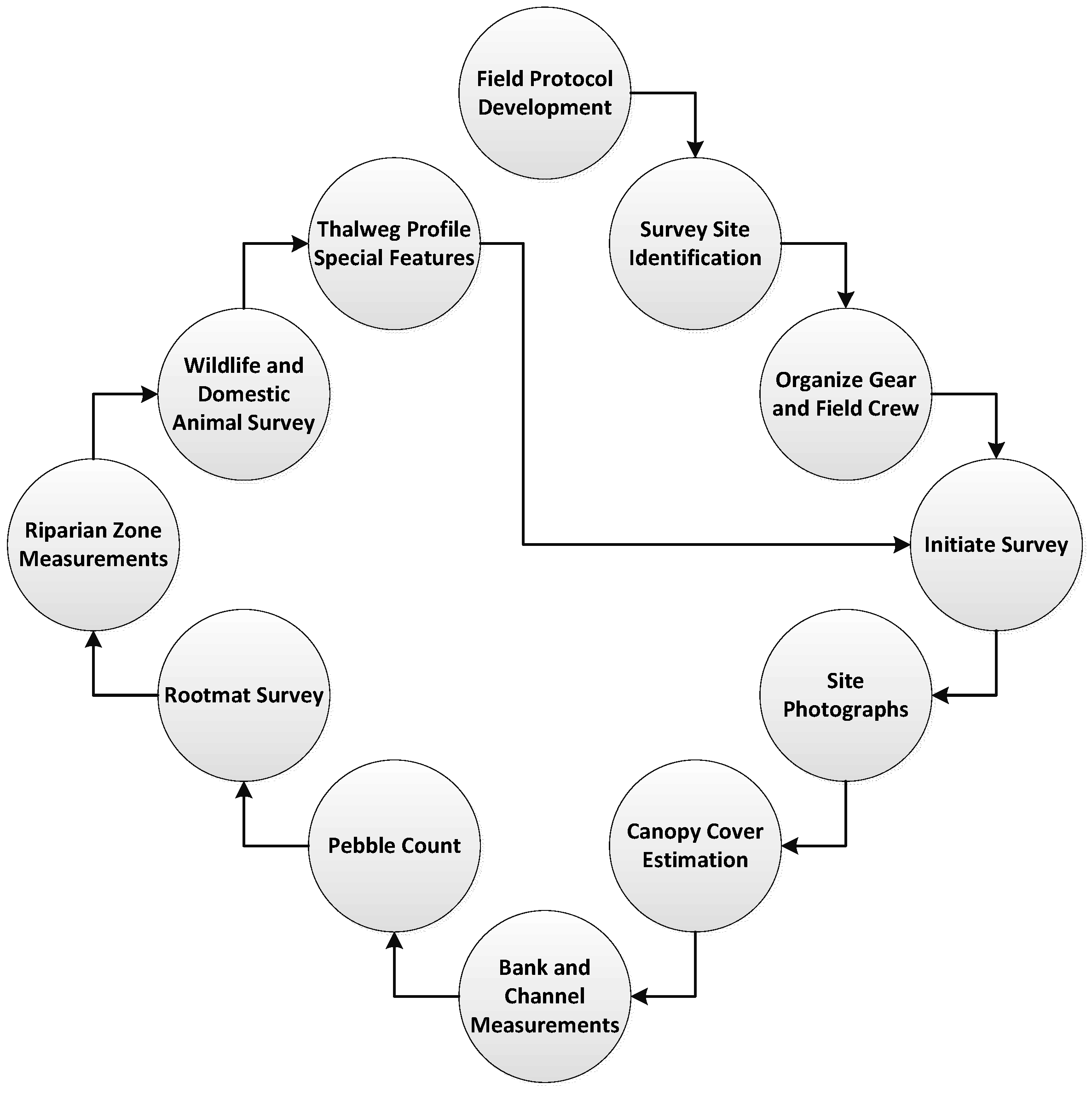
The rapid physical habitat assessment (rPHA) methods presented here can be conducted at any spatial or temporal frequency. Temporal frequency can be determined by establishing the amount of time, labor and financial support available to collect the desired information. The following protocol is flexible so that information can be collected along the entire length of a stream, and/or at points identified by observation, or using Geographic Information Systems (GIS) or other spatial technology. The utility of GIS frees the field crew from some traditional stream reach and stream width calculations. The spacing of the survey points will depend upon the goals of the researchers conducting the study and the length of the stream. For the study referenced in this article, the stream was 56 km long. It was determined that spacing survey points at 100 m intervals was appropriate and obtainable. A conceptual diagram of steps of the rPHA may assist the reader in understanding the work flow (
Figure 1). The following protocol assumes a field crew of at least three individuals, though it is recognized that field crew numbers may vary depending on available funds and desired outcomes. Thus, the assessment could be conducted by one or more individuals with only minor adjustments. Data collection criteria are presented in the order that they may logically occur during a field survey, though the order of field operations may also vary by site, application, and expectations. Field surveys should be conducted at or near baseflow conditions in the study stream to assure conveyance, and moving in an upstream direction to avoid clouding the survey area with disturbed sediment.
2.1. Identifying Survey Locations
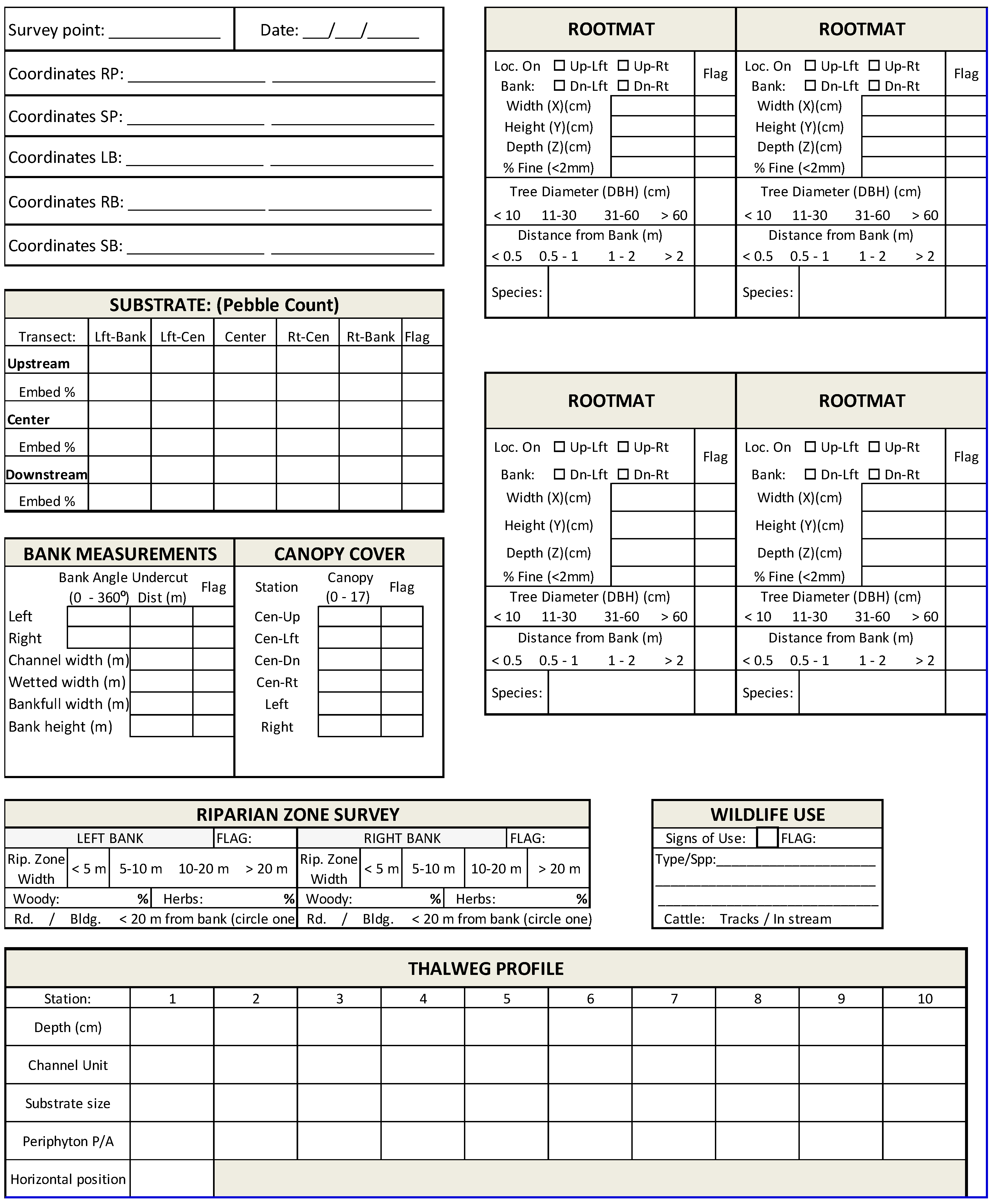
Prior to the field campaign, coordinates for each survey location should be numbered consecutively from the mouth to the headwaters of the study stream, or vice versa. Flow conditions in the study stream may prevent sequentially surveying the points, and pre-numbering the points prevents confusion about which points have been surveyed. It is recommended that GPS waypoints be named using a code for the survey point number. For example, the waypoint for survey point one could be named SP1 (Survey Point 1). Survey point numbers should be recorded on field data sheets (see example in
Appendix A) for later inputting to an electronic database along with the corresponding field measurements.
Survey points should be determined using standard ArcGIS or other spatial analysis software and preloaded into a Global Positioning System (GPS) handheld unit for use by the field team. In the field the project team may need to triangulate the survey position to the center of the stream channel closest to the preloaded coordinates because the GPS signal may be diminished or distorted in the stream channel due to topographic relief and/or vegetated canopy cover. For each point surveyed the data sheet should include the coordinates of the survey point (center of channel) and a set of coordinates at the center of the stream if different from the center of the channel. In addition, coordinates should be collected to mark the position of both stream banks (bottom of bank/top of stream bed gravel) on either side of each survey point. Coordinates of special features including woody debris piles, public utilities, engineered structures, erosion gullies, bank failures, debris piles, and any other obvious habitat altering features can also be recorded on the field data sheet or in the properties of photographs of the features if a camera that records GPS coordinates is used (see
Section 2.4). Collection of multiple sets of coordinates facilitates detailed mapping of the survey site locations if desired. Additional survey points can be established at the confluence of each of the major tributary of the study stream. Coordinates should be collected at confluence survey points (a set of coordinates at each of three transects—see
Section 2.2) and recorded in the same manner as the standard survey points.
2.2. Developing Study Plot Locations in the Field
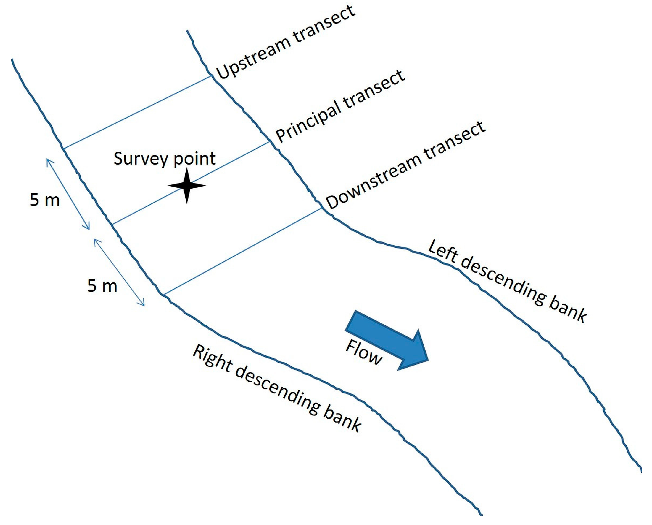
For the purposes of conducting measurements at each survey point (stream channel center), it may be useful to conceptualize the survey point as the center of a study plot. The study plot consists of a principal transect running from streambank to streambank through the survey point perpendicular to the direction of stream flow, bracketed by upstream and downstream transects located 5 meters from and parallel to the principal transect (
Figure 2).
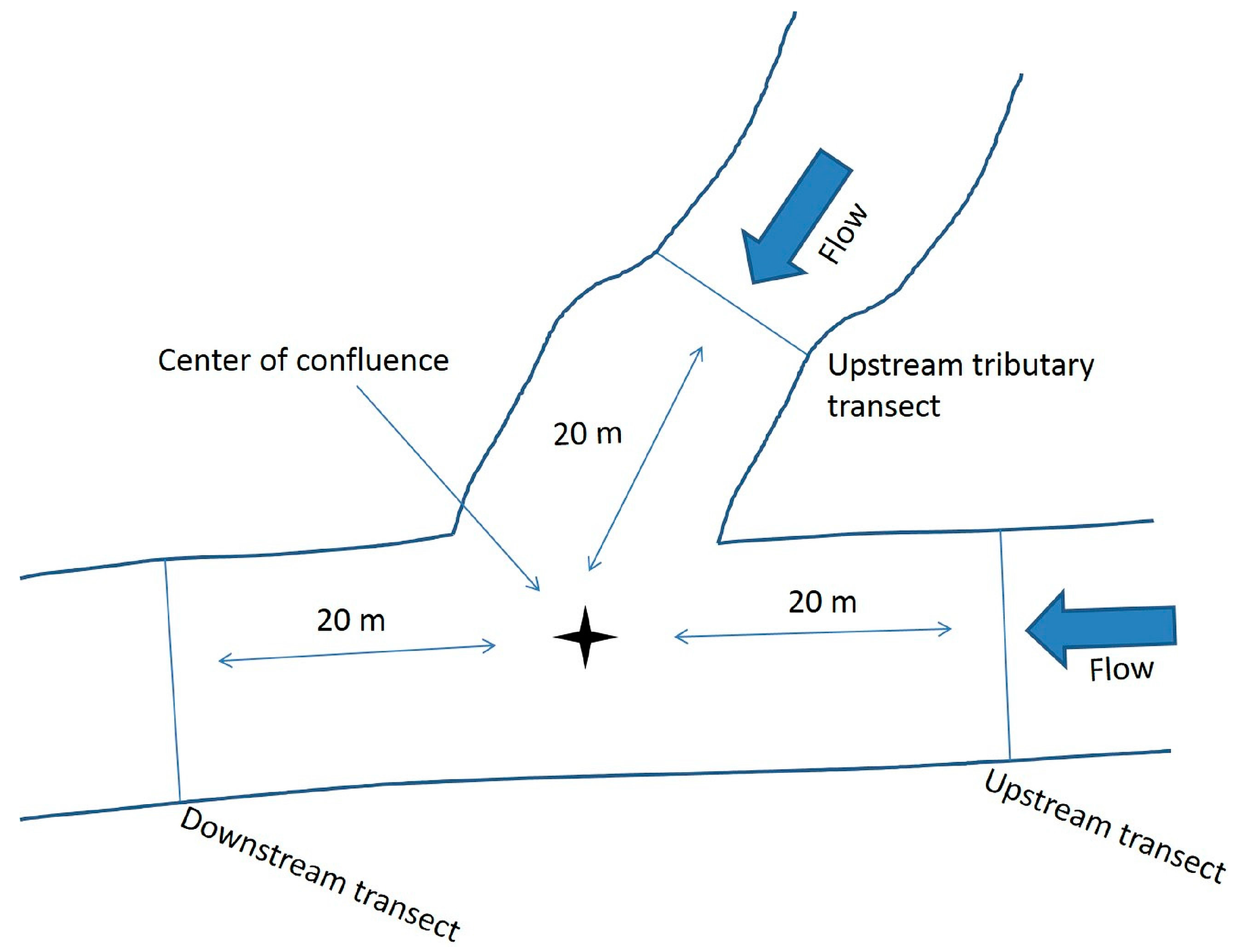
At confluences, the field team should create three transects: one upstream of the confluence in the study stream, one downstream of the confluence in the study stream, and a third upstream
in the tributary. Three transects established in this manner will more appropriately describe the characteristics of physical habitat at rapidly changing, dynamic locations (such as confluences). The three transects should be located equidistant from the center point of the confluence (
Figure 3). The distance measured from the center point of the confluence will depend upon the size of the channel at the confluence. The selected distance should locate transects on the study stream and the tributary at least 10 m upstream (the figure uses 20 m as an example) of the point where the upstream tributary bank and study stream intersect. All measurements described in this protocol should be collected along each of the three transects.
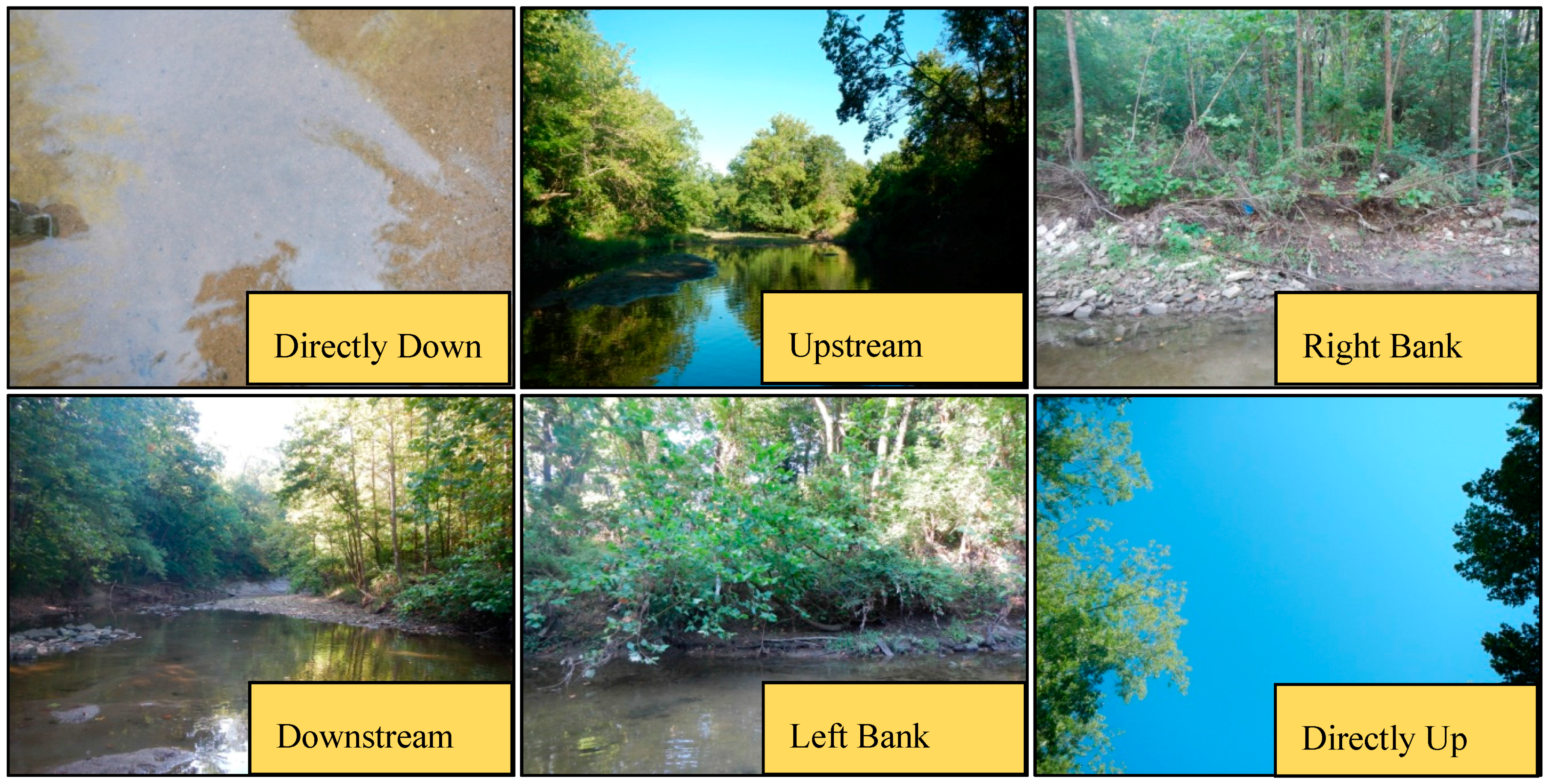
2.3. Photographic Database
A digital camera should be used to create a photographic database documenting each study plot. The set of photographs for each survey point is useful for comparison with photographs taken during subsequent rPHA resurveys of the same point. Use of a camera that records GPS coordinates is recommended so that coordinates of special features do not have to be read from a GPS and recorded on the data sheet. A standard set of photographs should be taken from the survey point in a consistent order for ease of cataloging. For example, directly down at a distance of 1 m from the stream bed (stream bed composition), directly upstream (parallel with the channel), then turning clockwise a perpendicular (90 degree angle) photograph of the left bank, directly downstream (parallel with the channel), a perpendicular photograph of the right bank, and a final photo directly upwards to capture canopy cover (
Figure 4). When possible, photographs of the stream banks should capture the extent of vegetative cover present.
At confluence survey points, the standard channel photographs described above should be collected, plus additional photographs to document any distinct physical characteristics at the confluence including a 360-degree panorama from the center of the confluence and at each of the three transects surveyed.
2.4. Special Features
If a GPS-enabled digital camera is used, GPS coordinates will be embedded in the properties of the photographs, thus documenting the presence and location of any of the following special features: bank stabilization structures, including rip-rap, gabion baskets, and other engineered structures; pipes, outfalls, discharge control structures, and utilities with any related infrastructures; disturbance features including erosion gullies, debris fans, slumps, bank failures, and woody debris piles; large trash dumps in or near the stream; other special features of interest in the study stream.
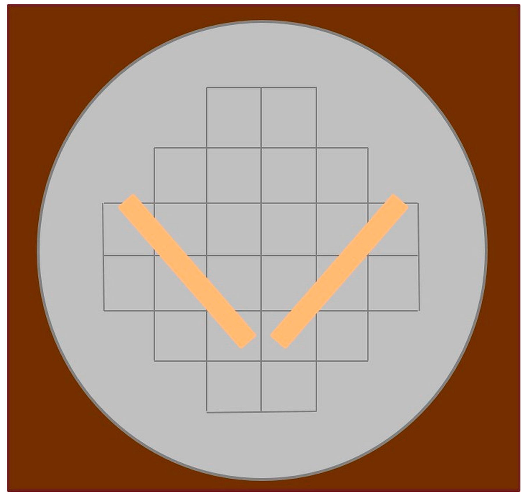
2.5. Estimating Canopy Cover
Canopy cover (proxy for stream shading) can be estimated following the method described by [
6] using a convex densiometer [
19] with a slight modification to prevent duplication of canopy cover from closely neighboring measurements. The modification consists of creating a “V” comprised of tape on the face of the densiometer with the vertex pointing towards the viewer so that 17 line intersections exist within the “V” [
20] (
Figure 5). The number of line intersections covered by canopy is recorded on the data sheet. During winter months, in deciduous cover, the number of line intersections covered by branches is recorded on the data sheet, and a notation is made as to the presence or absence of leaves. Canopy cover is determined by quantifying the percentage of points covered by canopy [
6], and as per the following procedure:
A field team member stands on the principal transect at mid channel facing upstream.
The densiometer is positioned 1 m above the stream bed, and leveled using the bubble level. The densiometer is then positioned so that the face of the field team member is reflected just below the apex of the taped “V” (
Figure 5).
The number of grid intersection points within the “V” that are covered by a tree, a leaf, or a high branch are counted (0 to 17) and recorded on the field data sheet (
Appendix A).
The field team member then faces the left descending bank (left, facing downstream). Steps 2 and 3 are repeated, and the value is recorded.
Steps 2 and 3 are repeated again facing downstream and again facing the right bank, and the values are recorded.
Steps 2 and 3 are repeated at the channel’s edge along the left bank (while facing the center of the stream) at the end of the principal transect, and again on the right bank, and the values are recorded.
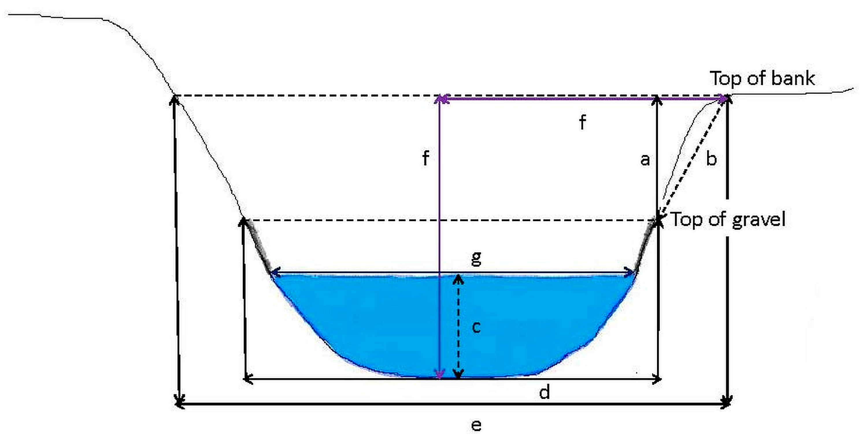
2.6. Bank and Channel Measurements
At each survey point, measurements of channel width, wetted width of the stream, bankfull width, bank angle, bank height, and channel depth should be recorded (
Figure 6). Bank angle is measured on both banks and calculated as the average slope of the bank extending a short distance from the bottom toward the top of the bank. A 1 m pole and clinometer can be used to measure bank angle. However, where the bank slope is variable or channels are incised, the use of a 2 m pole to average bank slope is recommended. It is further recommended that the top of the stream bed gravel be used to mark the bottom of the bank. The surface of the water can be used as bottom of the bank, but if the water level is ephemeral, the stream bed gravel (embedded in the stream bank) may be stable for longer periods of time and thus be a more reliable point of reference. Normally, slope is between 0° and 90°; however, by definition undercut banks have an angle greater than 90° because the edge of the water is underneath the overhanging bank. For comparison of all slope measurements collected during a rPHA, undercut banks should be measured from the water’s edge along the underside of the undercut, and the clinometers reading can be subtracted from 180° and recorded.
Identifying bankfull can be a challenge. Bankfull flows are of sufficient magnitude and velocity to erode the stream bed and stream banks, and frequent enough to prevent substantial regrowth of terrestrial vegetation after scouring [
6]. Annual peak flows are used to compare channel morphology measurements on a consistent basis, relative to bankfull flows thought to have a consistent 1.5–2.0-year return interval [
21]. Common indicators of bankfull level include the top of pointbars, changes in vegetation from aquatic to terrestrial, changes in slope, changes in bank material (e.g., from coarse gravel to sand), bank undercuts, or stain lines on bedrock or boulders [
22]. Determination of bankfull levels may require some discussion among crew members and if possible, multiple indicators that agree with each other should be used. Bankfull width can be measured as the distance between banks at the bankfull level perpendicular to stream flow. Bankfull bank refers to the bank with the lowest vertical distance from the surface of the water (i.e., the first to be breached in a high flow event). All measurements in this section with the exception of bank angle and channel depth can be made using a laser level and/or laser range finder. Bank angle can be determined using an extension pole, and locating the bottom of the stream bank at the top of the stream bed gravel (modified after [
6]):
An extension pole should be laid on the bankfull bank at the end of the principal transect so that the base of the pole is at the bottom of the bank (top of the line of coarse gravel from the stream bed). The extension pole is extended 2 m up toward the top of the bank. A clinometer is placed on the extension pole and the bank angle is recorded in degrees (0°–90°). If the bank is undercut (>90°), the measurement is made from the water’s edge along the underside of the undercut, and the clinometers reading is subtracted from 180° and recorded.
If the bank is undercut, the undercut depth is recorded by placing a meter stick horizontally parallel to the stream, and the distance from the back of the undercut to the edge of the bank is measured.
If there is a large boulder or log at the transect point, the measurement point should be moved (≤5 m) to a nearby point which is more representative of the slope of the bank.
Step 1 (and Step 2 if necessary) are repeated on the opposite bank.
Channel width, wetted width, bankfull width, bank height, channel depth, and relative thalweg depth and thalweg position are determined by the following procedure using a laser level and laser range finder to increase the speed of field measurements. A small amount of stream bank vegetation may need to be removed to prevent obstruction of the laser level and laser range finder:
Using a laser range finder, the distance from the bottom of the bank (the top of the gravel from the stream bed) is measured across the stream channel from one bank to the other (channel width), and the distance from one side of the stream to the other (wetted width) is measured. A meter stick is used to measure the wetted width manually if the width is below the lower end of the range of the laser range finder. If there is a split in the channel due to a bar or island, the following wetted width values are recorded where possible and applicable: entire width of wetted portion of the stream, wetted width nearest to left bank, wetted width of center stream channel, wetted width nearest to right bank. Values for channel width and wetted width(s) should be recorded on the data sheet.
To measure bankfull width, the bankfull level on the stream bank with the highest terrace is located (please see discussion above or [
21] for more information). From the top of the stream bank with the lowest terrace (bankfull bank), a field team member can use the laser range finder (visually leveled with the level inside of the device) to measure the width to the bankfull level on the opposite stream bank.
Whether the right bank or left bank (descending) is used for bank measurements is determined at each survey point by which bank has the lower elevation (bankfull bank), and is noted on the data sheet. Bank height is measured as the distance from the bottom of the bankfull bank (determined by the top of the line of gravel from the stream bed) to the top of the stream bank. A laser level (transmitter) is placed at the top of the bankfull bank and a field team member standing in the stream bed extends an extension pole with a receiver attached upward (in a vertical position) from the bottom of the bankfull bank. The receiver makes intermittent beeping noises when it gets close to the horizontal plane of the projection from the laser level transmitter; the beeping noises become a continuous sound once bank height is reached. Bank height measurements should be adjusted in spreadsheet to subtract the height from the bottom of the laser level transmitter to the point where the laser beam is emitted.
Thalweg depth is measured by positioning the meter stick or extension pole on the stream bed at the deepest part of the channel and reading the depth of the water. In the event that the water is more than chest deep, a float with a depth finder can be deployed to measure thalweg depth.
Thalweg depth and thalweg position are measured relative to the bankfull bank. Relative thalweg depth is measured in a manner similar to bank height, using the laser level as a transmitter and an extension pole with a receiver. The extension pole is set at the bottom of the stream in the thalweg, and raised or lowered in a vertical position until the receiver is on a horizontal plane with the laser level transmitter stationed at the top of the bank (
Figure 6). Relative thalweg depth measurements are adjusted in spreadsheet to subtract the height from the bottom of the laser level transmitter to the point where the laser beam is emitted. Thalweg position is measured using a laser range finder to measure the distance between the top of the bankfull bank and the laser receiver on the extension pole. In water deeper than chest deep, an inner tube or other flotation device can be used to float near the thalweg of the stream to obtain the measurements.
2.7. Longitudinal Thalweg Depth Profile
The thalweg is the path of the stream that follows the deepest point of the channel [
23]. This is also the last part of the channel to become dry during low flow conditions. Although this is not a bathymetric profile, a longitudinal profile of thalweg depth yields information about potential habitat complexity and channel form variability. Here, the thalweg is measured at each survey point and every 10 m between survey points, however, measurement point distances could vary depending on the application and desired study outcomes. At the location of each thalweg measurement (including position 1, the survey point) a field crew member records the thalweg depth and the channel unit code (
Table 1).
The thalweg profile is determined by the following procedure (modified from [
6]). 10 m intervals were selected here given the 100 m distance between survey points. However, this distance can be modified:
Using a string line marked at 10 m intervals and run for 90 m from the survey point, the field team travels upstream following the thalweg.
At each 10 m interval, the depth of the water is measured at the deepest part of the channel in the same manner that thalweg depth is measured at the survey points. This depth (cm) is recorded under the appropriate station number on the data sheet.
At each 10 m point, the channel unit is identified and the channel unit code is recorded on the data sheet.
2.8. Substrate Characterization (Pebble Count)
At each thalweg measurement after the survey point (i.e., positions 2 through 10), the substrate size classification of a randomly selected particle is recorded (
Table 2), as well as the presence or absence of periphyton on the selected particle. It is acknowledged that pebble counts may not always be the most precise method of substrate characterization. However, this method was chosen here because it remains highly informative, is less costly, and much less time-consuming relative to other methods, a review of which is beyond the scope of the current article. Periphyton on rock surfaces can provide habitat for micro-organisms and some macroinvertebrates, and can provide refugia for these organisms from high velocity flows [
24]. Periphyton presence is also an indicator of stream productivity [
25,
26]. This procedure yields estimations of the diameter size class of 15 substrate particles at each study plot (adapted and modified from [
6,
27]). Five particles each are selected from the principal transect, the upstream transect, and the downstream transect (
Figure 2). At each transect, particles are samples from the left and right banks, and from 25%, 50%, and 75% of the distance across the width of the channel. Particle size is then estimated according to the size classes listed in
Table 2. Much of the time savings of the rPHA method presented in this work occurs at this point by collecting only 15 substrate particles instead of 100 particles recommended by [
27]. As with other parameters, this method can also be modified to best suit specific needs. Where possible the presence or absence of periphyton on the substrate particle at the thalweg should be determined and noted on the data sheet.
Substrate measurement is conducted as follows:
Beginning on a bank of the principal transect, a field team member randomly points to a spot on the channel bed using a meter stick. The first particle that the meter stick comes into contact with is selected. If the substrate is sand or finer material, multiple particles are picked up and size class is determined by texture.
The size of the selected particle is estimated (or particles for finer material) as per
Table 2.
The percent vertical embeddedness of the particle in the substrate (what percentage of the particle is not visible) is estimated to the nearest 5%. Sand and silt are by definition 100% embedded, and bedrock or claypan are 0% embedded.
The field team member moves to the next station along the principal transect (stream bank, 25% across channel width, 50% across channel width, 75% across channel width, stream bank) and repeats Steps 2 to 3. Five particles are sampled on the principal transect.
Steps 1 to 3 are repeated on the upstream transect and the downstream transect (
Figure 2), for a total of 15 particles per study plot.
2.9. Rootmat Survey
Submerged woody rootmats are important refugia for aquatic macroinvertebrates [
28]. The following method can be used to quantify the volume and density of root habitat and characterize the composition of riparian vegetation which may be important to rootmat availability [
11].
Any submerged woody rootmats within the study plot are located. The following procedures are repeated separately for each separate contiguous area of rootmat within the study plot (
Figure 2). A single tree may have more than one separate rootmat. Likewise, a single contiguous rootmat is sometimes composed of the roots from multiple trees. The position of each rootmat relative to the principal transect is recorded and the location on the stream bank is noted by checking the box next to the appropriate category on the data sheet (e.g., “Up-Lft” refers to the left bank upstream of the principal transect, and “Dn-Rt” refers to the right bank downstream of the principal transect).
To calculate the volume of submerged rootmats, each contiguous area of rootmat should be measured in three dimensions (parallel to bank, perpendicular to bank, and vertical). Each of the three measurements is recorded on the data sheet. For large contiguous rootmats, a laser range finder may be used to measure the length of the rootmat parallel to the bank, otherwise a meter stick is the appropriate tool.
The percent by volume of fine roots is visually estimated (<2 mm diameter) to the nearest 10%.
The parent species of tree or shrub is recorded. In cases where there are multiple parent trees or shrubs, each species is recorded. In cases where the exact parent tree cannot be determined, the dominant or most abundant species within a 2 m radius is recorded.
The diameter at breast height (DBH) of each parent tree is estimated according to predetermined size classes. Size classes are <10 cm, 11–30 cm, 30–60 cm, >60 cm. The appropriate DBH value is circled on the data sheet. If the parent tree cannot be determined, “N/A” should be circled.
Linear distance from the base of the tree to the edge of the top of the bank is estimated according to predetermined ranges (for example, <0.5 m, 0.5–1 m, 1–2 m, and >2 m).
2.10. Riparian Zone Assessment and Determination of Dominant Vegetation Type
The width of the riparian corridor and dominant vegetation type may be used to assess what areas of the study stream might be impacted by excessive runoff, bank erosion, and/or sedimentation during high flow events. This information, in combination with other quantitative assessments, can be used to assess stream ecosystems and may assist in future decisions regarding re-vegetation, bank stabilization, or other management projects [
29,
30].
A visual estimation is made of the width of the riparian zone of each bank and recorded as one of several classes: 0–5 m, 5–10 m, 10–20 m, >20 m. Riparian vegetation includes trees, grasses, and sparse vegetation, but does not include vegetation identifiable as crops or lawn grass. The presence of any fencing, roads or buildings in the riparian zone is noted including the approximate distance from the stream bank. A visual estimation of the mix of woody and herbaceous vegetation types in the riparian zone is made, and classified as a percent mix of the two classes, i.e., 60% woody, 40% herbaceous.
2.11. Wildlife and Cattle
If wildlife and/or domestic animals (e.g., cattle, horses, goats, etc.) have access to the study stream (and can be identified using tracks or other methods) this should be documented. The use of the study stream by domestic livestock (and potentially wildlife) may impact the suspended sediment load [
31], and levels of bacteria such as
Escherichia coli (
E. coli) [
32]. A visual survey is conducted at and between survey points. Presence or absence of wildlife use is recorded. If wildlife is observed, the type of wildlife is noted (including species, if known). If animal tracks are present at the survey point or along the upstream distance between survey points, they are identified using an animal track field guide, and recorded on the data sheet.
3. Data Analysis
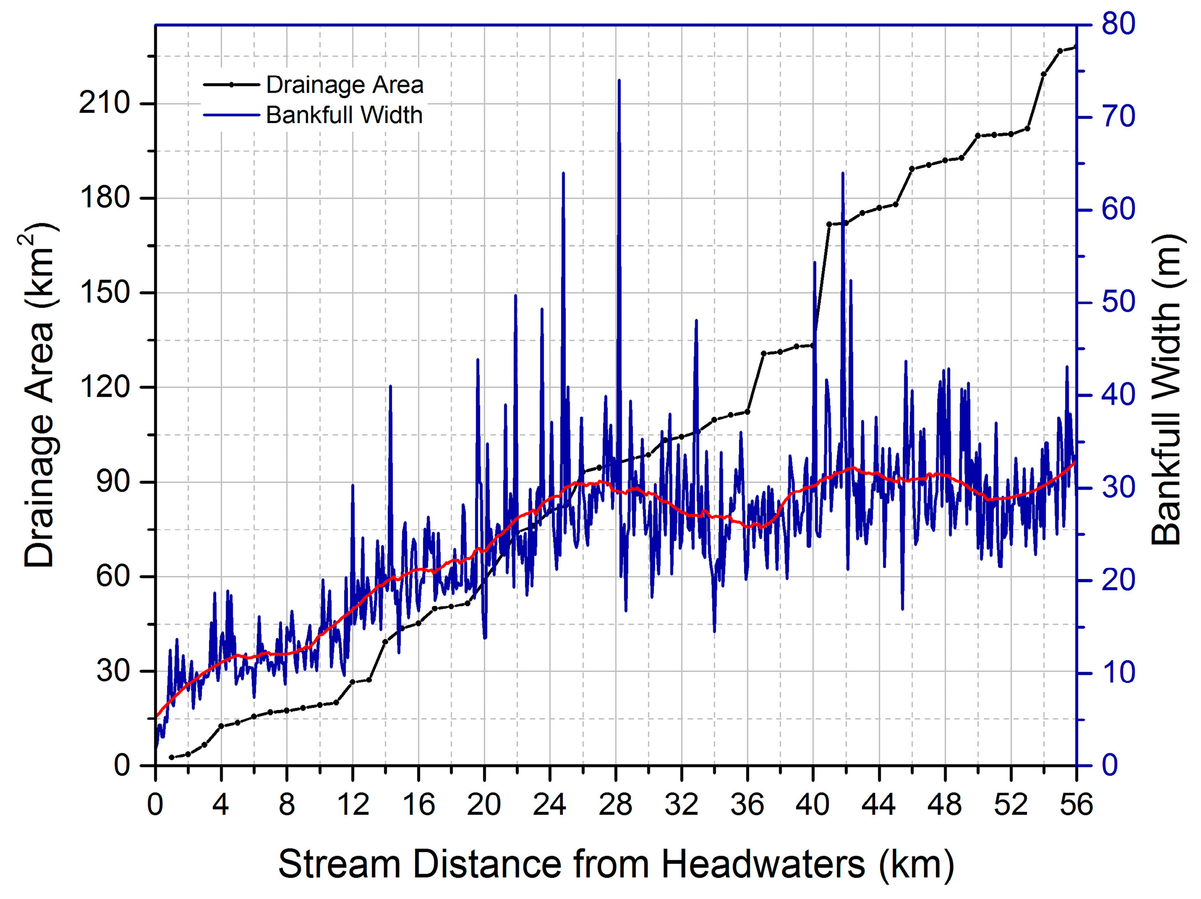
Preliminary analysis of rPHA data should begin by calculating descriptive statistics of the data for the length of the stream, including (but not limited to) mean, minimum, maximum, standard deviation, coefficient of variation, etc., to describe the basic features of the data. This process will provide simple summaries about the sample and the measures and should be followed by graphing individual stream metrics against various landscape features such as roads and bridges. Where data points are highly variable, a moving average can be used in lieu of a trend line. Stream distance and drainage area are physiographic features that are useful to compare and contrast stream metrics, as well as land use in mixed-land-use watersheds. Land use can be determined using public resources such as the National Resources Inventory in conjunction with ArcGIS tools. Photographs collected during a rPHA will document the location of other features including small tributaries, bridges, and outfalls which may alter local hydrology and hydraulics, and these features can be mapped and graphed with stream metrics to examine the influence of localized features.
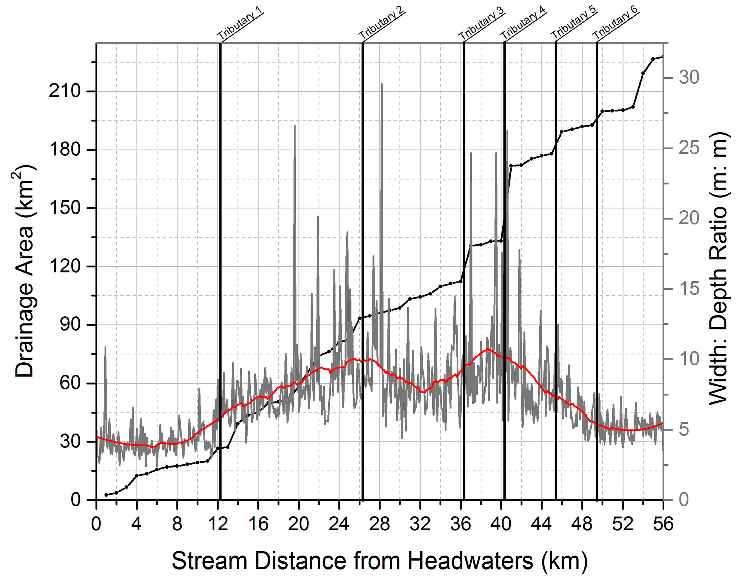
Figure 7 and
Figure 8 (using data from an rPHA of Hinkson Creek, Boone County, MO, USA) illustrate use of bankfull width data in different analyses. The location of major confluences is shown as an overlay in
Figure 8, and can be compared to stream distance, drainage area, and width to depth ratio among other variables. Stream distance and drainage area can be calculated using a combination of ArcGIS and ArcHydro tools. Digital elevation model (DEM) data of many if not most locations in the United States is publicly available and can be used to delineate watershed boundaries.
Selections of two or more metrics can be graphed with stream distance to model the combination longitudinally. For example, bank height and thalweg depth, two metrics which are important determinants of urban stream syndrome [
12], can be graphed together (surface of the water can be set at zero, with bank height as a positive
y-axis, and thalweg depth as a negative
y-axis) to analyze the relationship between the metrics with stream distance and drainage area. Additionally, natural stream constraints such as bedrock may be mapped and graphed to explore relationships with stream metrics individually or in combination.
Analyses of the data collected during the rPHA will vary depending upon the objectives and expertise of the investigators. A primary goal of the analysis should be to compare longitudinal differences in physical habitat metrics to determine whether there are variations from expected patterns and if so, where the variations occur. This relatively simple descriptive and visual analysis is often most useful for identifying beneficial locations for mitigation activities. For example, the bankfull width analysis shown in
Figure 7 exhibits very little variability in the 36 to 40 km range of the graph. With additional consideration (i.e., photographic database) it is apparent that this area of the stream is constrained by bedrock thus limiting the ability of the stream to adjust to upstream stressors. Another example may be seen in
Figure 8 where the steepness of the width:depth curve increases suddenly at approximately 40 km from the headwaters. Additional analysis reveals the influence of a large urban area (and potential accompanying urban stream syndrome [
12]) in the lower third of the watershed. As trends are noted in graphs of single or grouped metrics, multiple correspondence analyses may be used to determine the relative influence of individual metrics on stream physical habitat or to predict habitat suitable for aquatic biota. With clearly stated assumptions, multiple linear regression and principal component analysis are additional statistical techniques (see the literature for other techniques) that may be applied [
33,
34]. These techniques can be used to quantify and statistically assess the relative influence of various metrics and may help to prioritize features of the stream bed or channel to target in stream restoration efforts. Finally, given that rivers and streams are reflections of upland and instream processes and distance, the spatial and temporal inter-relationship of survey sites are arguably not independent [
35]. In fact, one benefit of the rPHA may be to illustrate where upstream sites are affecting those downstream due to any variety of factors including land use changes, the presence of woody debris, etc. The potential for autocorrelation of the data highlights the importance of the collection of information about special features during the rPHA (see
Section 2.4).
4. Conclusions
The use of biotic indices to identify impairment in streams may not provide useful information about causes of impairment, which may lead to unsuccessful mitigation strategies. A physical habitat assessment (PHA) can yield greater information about potential causes of impairment, particularly in mixed-land-use watersheds where multiple land use practices interact in complex ways to confound water quality mitigation attempts. Often, field work for a PHA can be time-consuming and labor intensive. The method described here provides a thorough, economical, science-based, rapid methodology achievable in low gradient, riffle-pool, mixed-use watersheds with limited or focused budgets. Physical habitat metrics were chosen based upon relevance in mixed-land-use systems, and the ability to compare expected variability with stream distance to actual measurements. The metrics selected are intended to provide a broad data set that characterizes the availability and condition of physical habitat in-stream (along the continuous length of the stream) as well as potential habitat available in the riparian corridor, while reducing time of collection and thereby reducing assessment cost. Other methods of data collection may be more revealing about stream physical habitat (and more costly), but the methods in the current rPHA provide a broad field-based dataset in a shorter fiscally responsive timeframe. The impetus for the current method paper was to demonstrate a rapid method that can serve as a practitioner’s management tool. For example, the pebble count method used here is just one of a set of simplified indices that collectively take a systems approach in relatively complex mixed-land-use watersheds. Many questions remain about the appropriate spatial scales for such surveys to yield cost-effective returns for managers and the greatest limiting factor, is often quantity of data. A saturation approach (higher number of data points in a smaller area), while perhaps not as precise, may be more spatially informative and within the bounds of necessary accuracy to achieve conservation goals. Data collected can be analyzed to inform understanding of stream response to stressors and help to identify sites with ongoing degradation, thereby supplying detailed information about variability in physical habitat characteristics at a range of spatial scales. After data analysis, repeated assessments at strategic “problem sites” can further inform the need for specific management actions. For example, the suite of photographs collected during the rPHA are a valuable source of data regarding stream conditions at a specific moment in time and may provide a simple comparative indices to future photographs. Temporal variability of rapid physical habitat assessment (rPHA) indices can be assessed at various intervals (e.g., three to five years in a rapidly changing system), thereby informing adaptive management efforts in streams with ongoing impacts and impairment. Collection of stream habitat data using the rPHA methods described here can provide site-specific data expeditiously, and at relatively low cost, resulting in a reduced cost, highly effective methodology to guide mitigation and restoration efforts.


