
Variability and Trends in Precipitation, Temperature and Drought Indices in the State of California

Abstract
:1. Introduction
2. Materials and Methods
2.1. Drought Indices
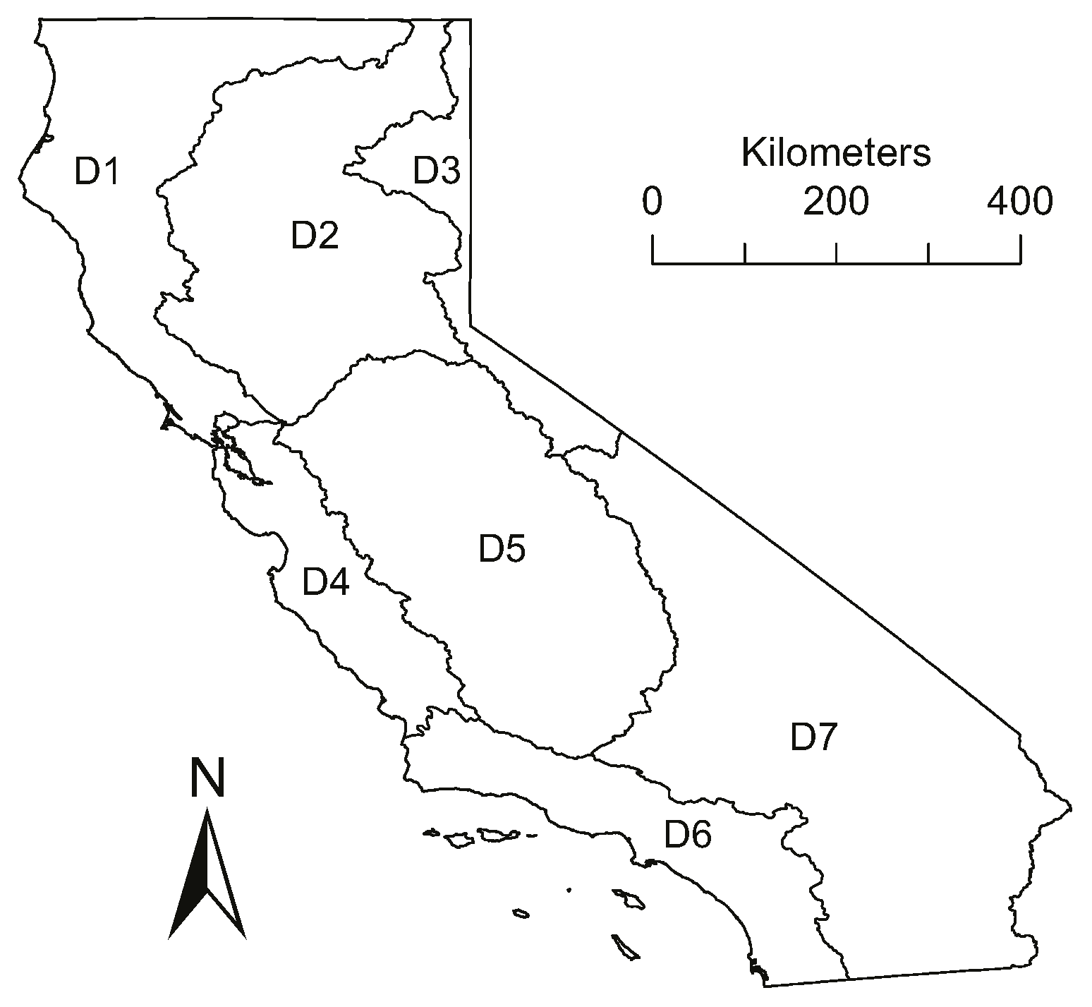
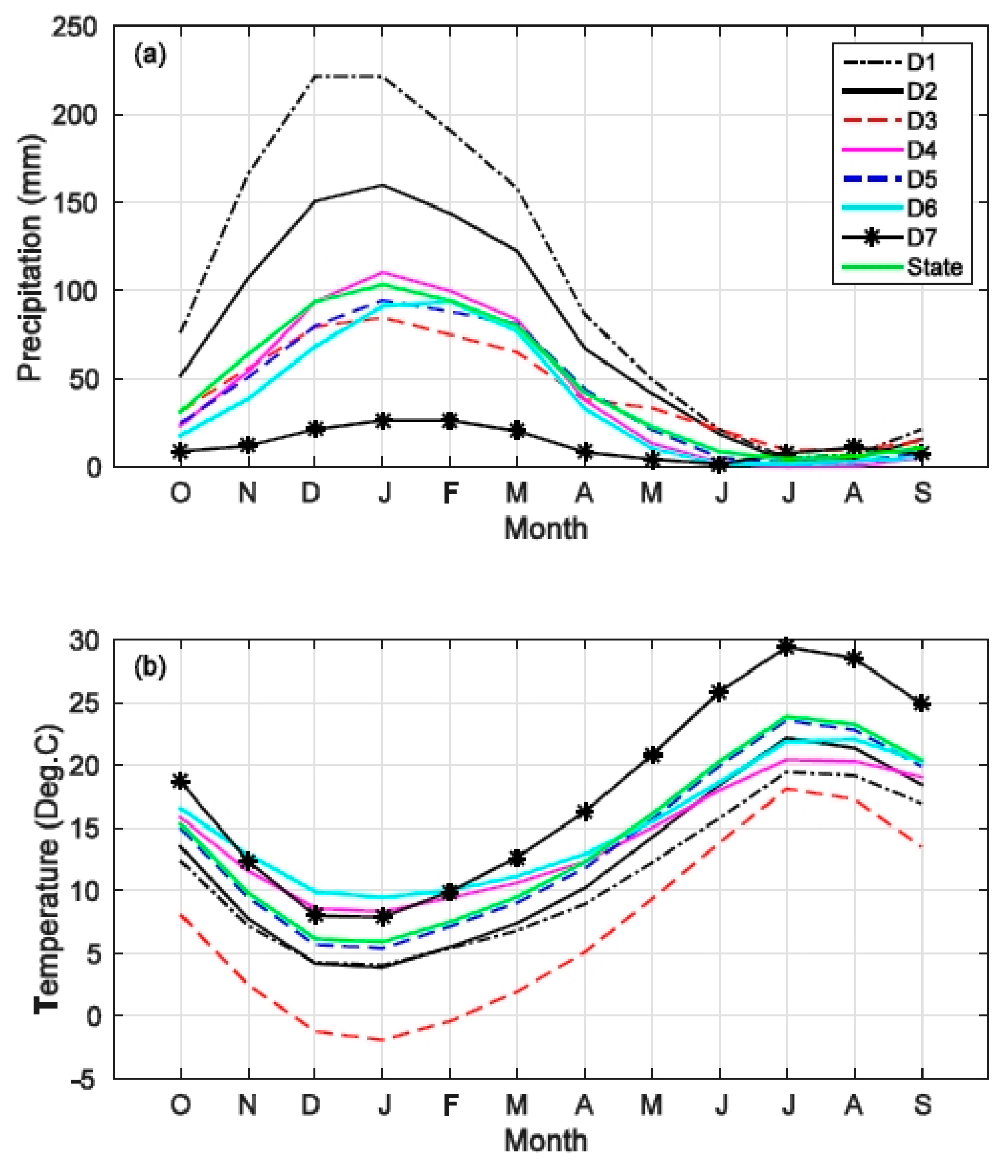
2.2. Study Area and Dataset
2.3. Metrics
2.4. Trend Analysis
3. Results
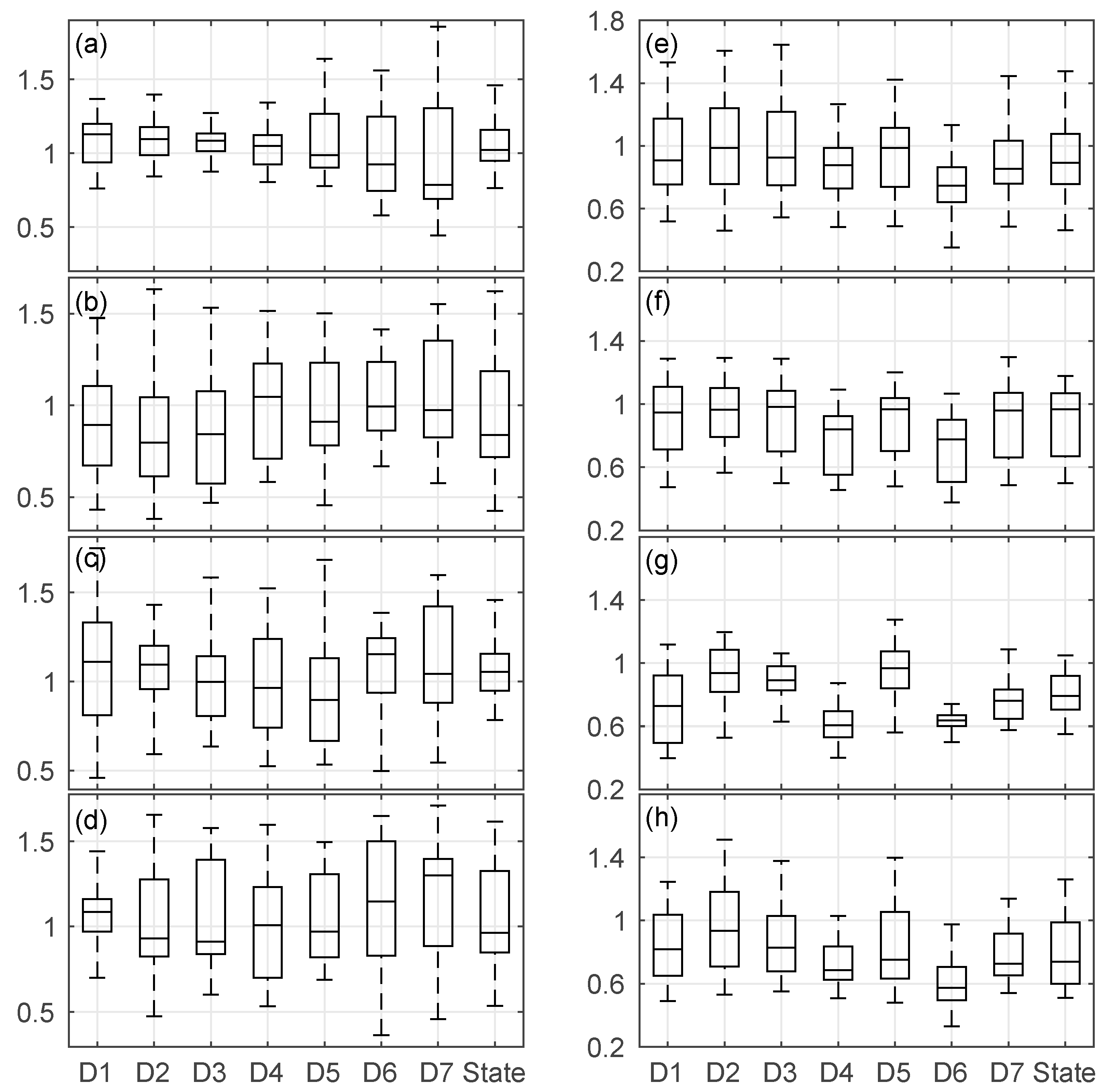
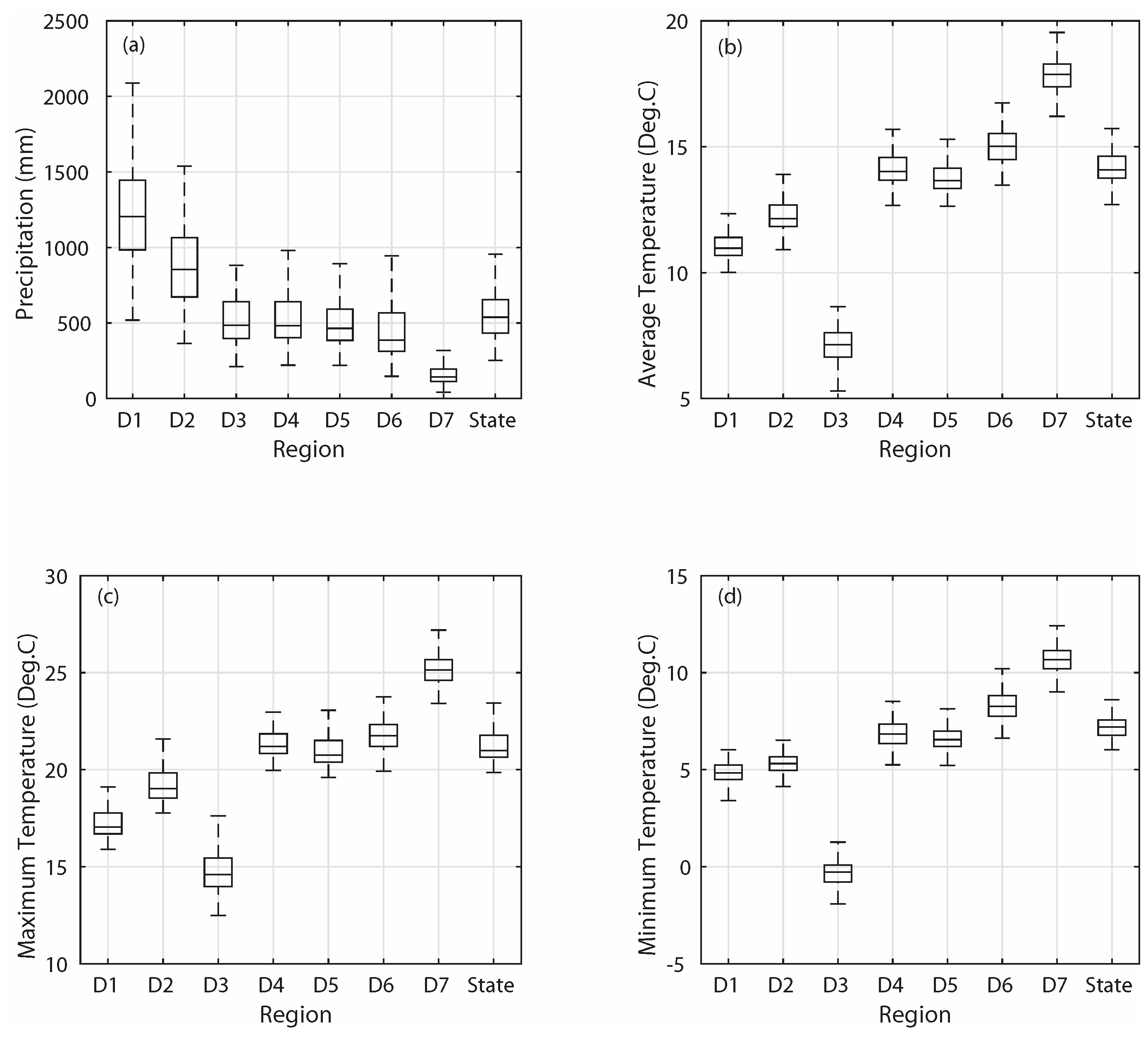
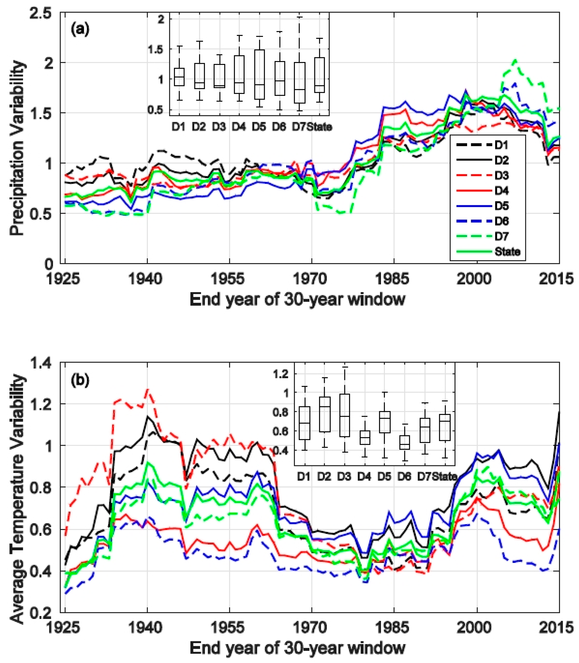
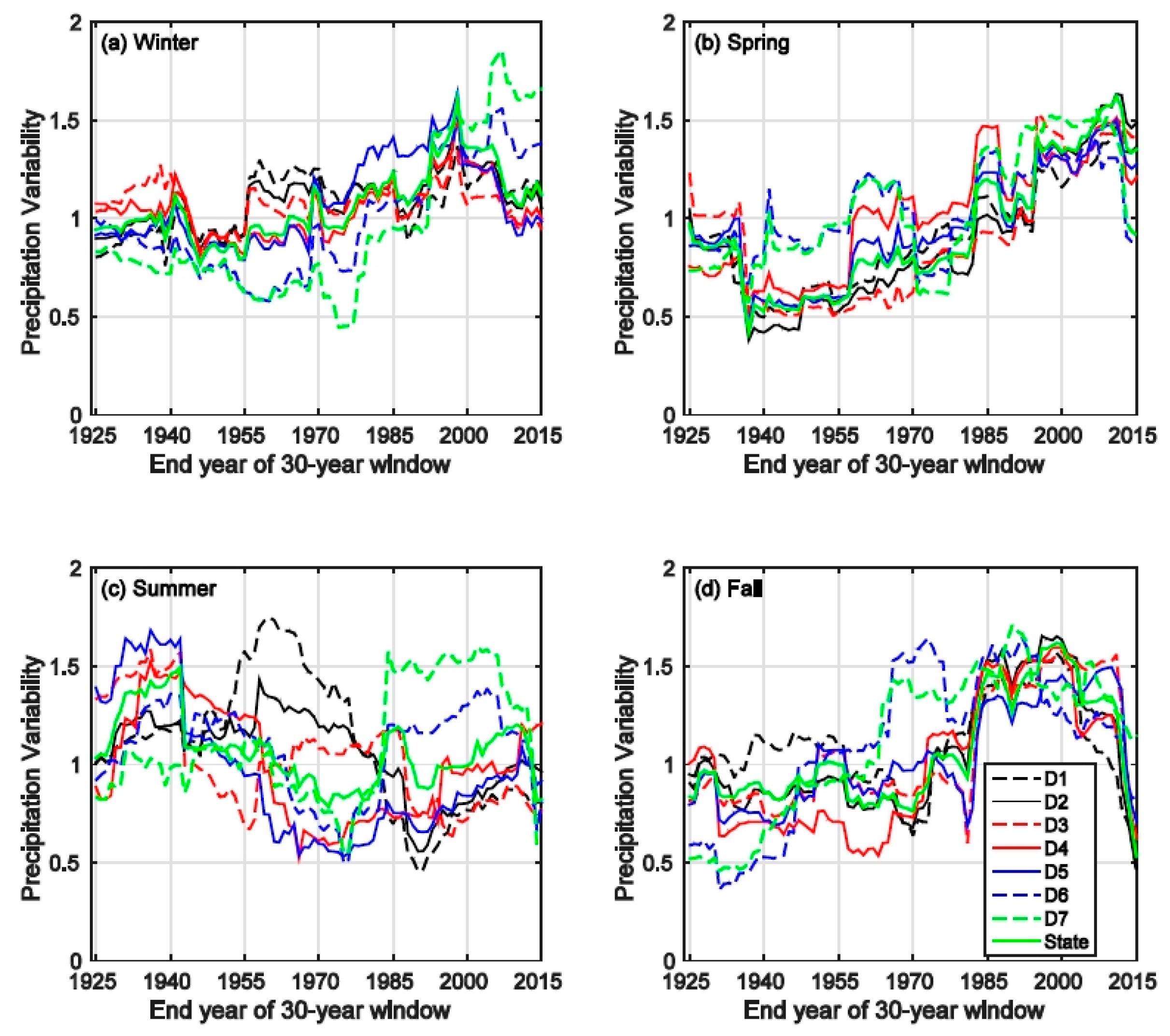
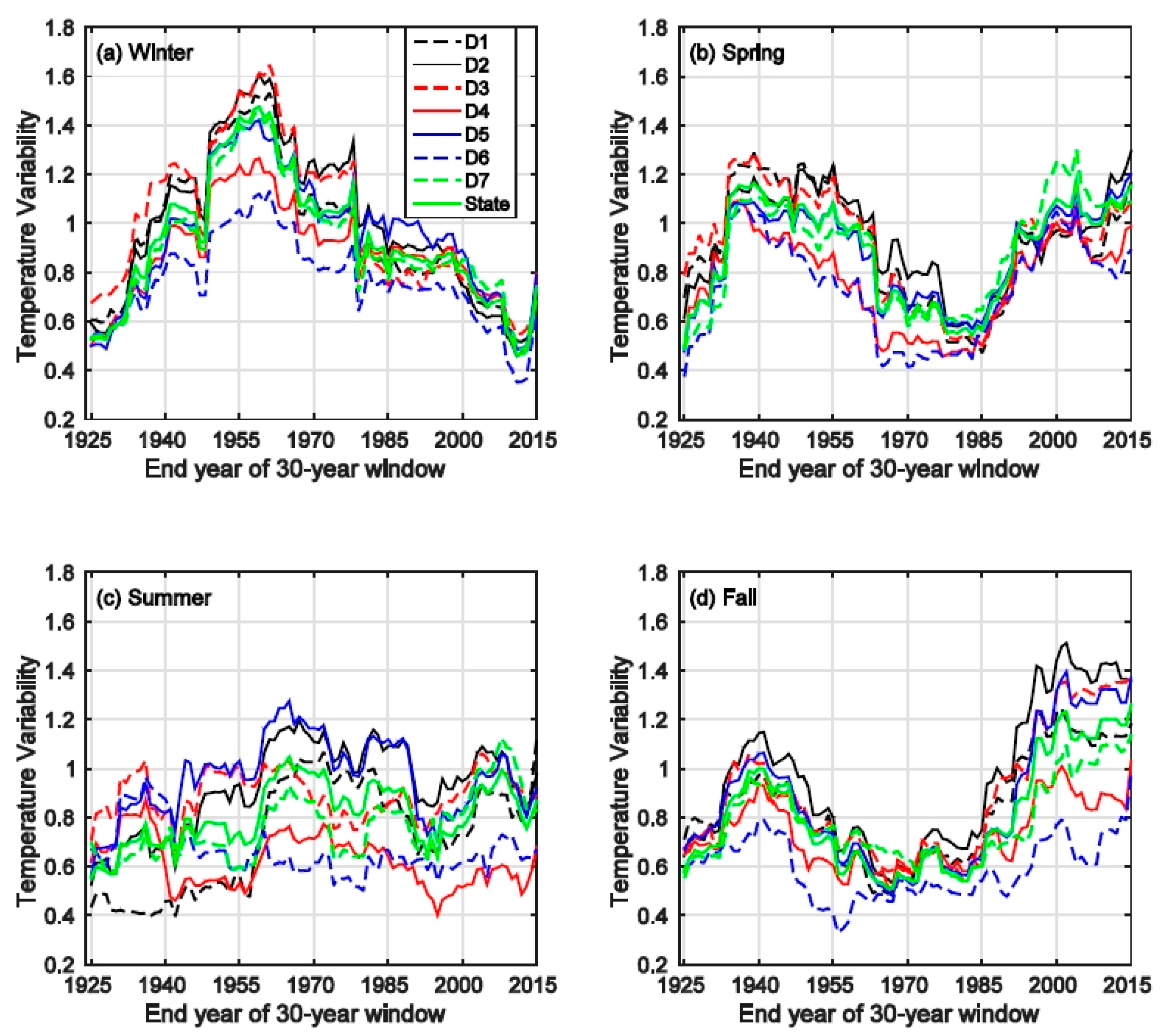
3.1. Variability
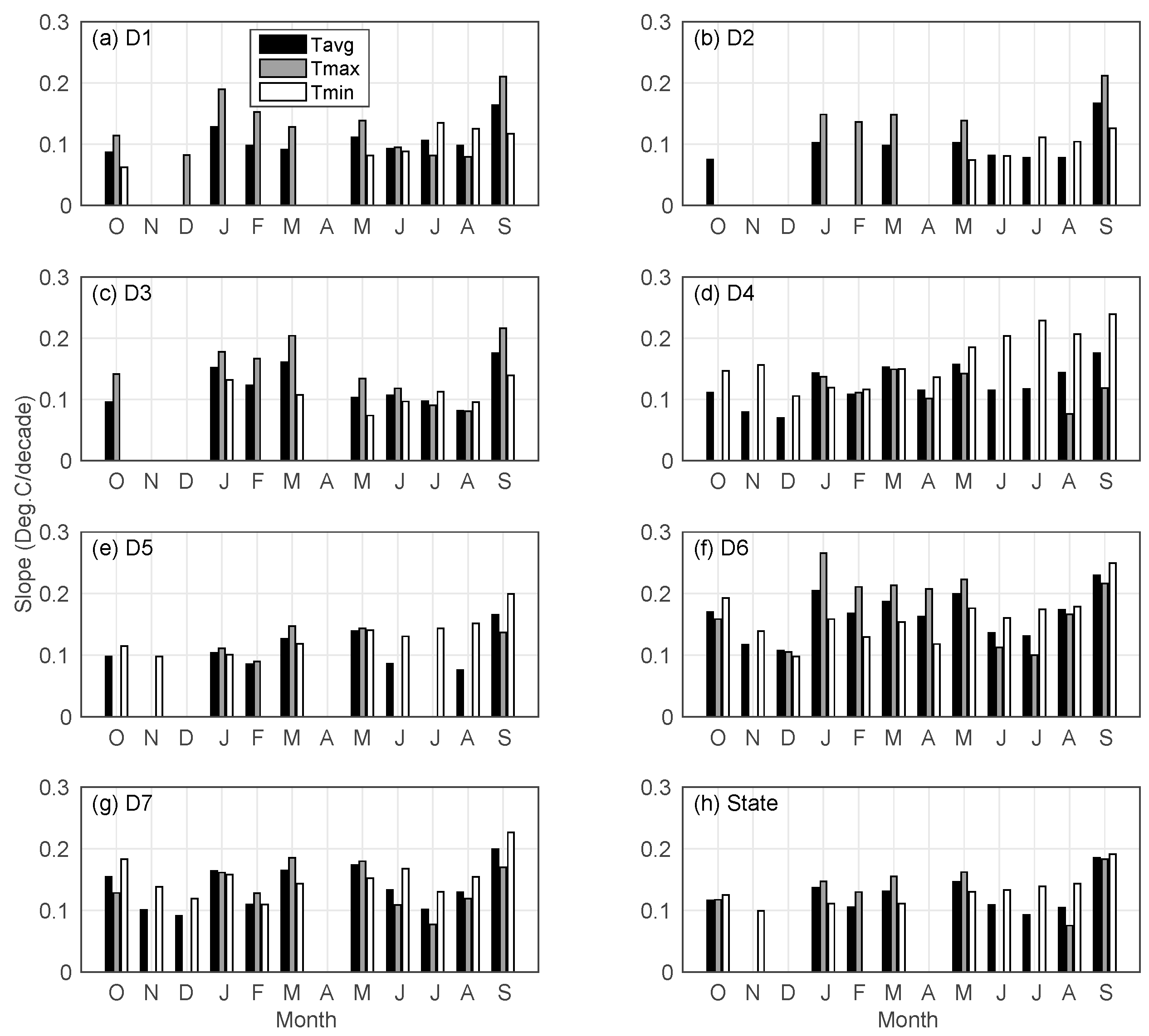
3.2. Trend
4. Discussion
5. Conclusions
Acknowledgments
Author Contributions
Conflicts of Interest
References
- Mote, P.W.; Hamlet, A.F.; Clark, M.P.; Lettenmaier, D.P. Declining mountain snowpack in western north america. Bull. Am. Meteorol. Soc. 2005, 86, 39–49. [Google Scholar] [CrossRef]
- Grundstein, A. Evaluation of climate change over the continental united states using a moisture index. Clim. Chang. 2009, 93, 103–115. [Google Scholar] [CrossRef]
- Pryor, S.; Howe, J.; Kunkel, K. How spatially coherent and statistically robust are temporal changes in extreme precipitation in the contiguous USA? Int. J. Climatol. 2009, 29, 31–45. [Google Scholar] [CrossRef]
- Grundstein, A.; Dowd, J. Trends in extreme apparent temperatures over the united states, 1949–2010. J. Appl. Meteorol. Clim. 2011, 50, 1650–1653. [Google Scholar] [CrossRef]
- Hoerling, M.P.; Dettinger, M.; Wolter, K.; Lukas, J.; Eischeid, J.; Nemani, R.; Liebmann, B.; Kunkel, K.E.; Kumar, A. Present weather and climate: Evolving conditions. In Assessment of Climate Change in the Southwest United States; Springer: Berlin, Germany, 2013; pp. 74–100. [Google Scholar]
- Schwartz, M.D.; Ault, T.R.; Betancourt, J.L. Spring onset variations and trends in the continental united states: Past and regional assessment using temperature-based indices. Int. J. Climatol. 2013, 33, 2917–2922. [Google Scholar] [CrossRef]
- Bonfils, C.; Duffy, P.B.; Santer, B.D.; Wigley, T.M.; Lobell, D.B.; Phillips, T.J.; Doutriaux, C. Identification of external influences on temperatures in california. Clim. Chang. 2008, 87, 43–55. [Google Scholar] [CrossRef]
- Bonfils, C.; Santer, B.D.; Pierce, D.W.; Hidalgo, H.G.; Bala, G.; Das, T.; Barnett, T.P.; Cayan, D.R.; Doutriaux, C.; Wood, A.W. Detection and attribution of temperature changes in the mountainous western united states. J. Clim. 2008, 21, 6404–6424. [Google Scholar] [CrossRef]
- Kunkel, K.; Stevens, L.; Stevens, S.; Sun, L.; Janssen, E.; Wuebbles, D.; Kruk, M.; Thomas, D.; Shulski, M.; Umphlett, N. Regional climate trends and scenarios for the us national climate assessment: Part 4. Climate of the us great plains. NOAA Tech. Rep. NESDIS 2013, 142, 91. [Google Scholar]
- Lavers, D.A.; Villarini, G. The contribution of atmospheric rivers to precipitation in europe and the united states. J. Hydrol. 2015, 522, 382–390. [Google Scholar] [CrossRef]
- Wang, H.; Schubert, S.; Suarez, M.; Chen, J.; Hoerling, M.; Kumar, A.; Pegion, P. Attribution of the seasonality and regionality in climate trends over the united states during 1950–2000. J. Clim. 2009, 22, 2571–2590. [Google Scholar] [CrossRef]
- Westby, R.M.; Lee, Y.-Y.; Black, R.X. Anomalous temperature regimes during the cool season: Long-term trends, low-frequency mode modulation, and representation in cmip5 simulations. J. Clim. 2013, 26, 9061–9076. [Google Scholar] [CrossRef]
- Cordero, E.C.; Kessomkiat, W.; Abatzoglou, J.; Mauget, S.A. The identification of distinct patterns in california temperature trends. Clim. Chang. 2011, 108, 357–382. [Google Scholar] [CrossRef]
- MacDonald, G.M. Water, climate change, and sustainability in the southwest. PNAS 2010, 107, 21256–21262. [Google Scholar] [CrossRef] [PubMed]
- McRoberts, D.B.; Nielsen-Gammon, J.W. A new homogenized climate division precipitation dataset for analysis of climate variability and climate change. J. Appl. Meteorol. Clim. 2011, 50, 1187–1199. [Google Scholar] [CrossRef]
- AghaKouchak, A.; Cheng, L.; Mazdiyasni, O.; Farahmand, A. Global warming and changes in risk of concurrent climate extremes: Insights from the 2014 california drought. Geophys. Res. Lett. 2014, 41, 8847–8852. [Google Scholar] [CrossRef]
- Cheng, L.; Hoerling, M.; AghaKouchak, A.; Livneh, B.; Quan, X.-W.; Eischeid, J. How has human-induced climate change affected california drought risk? J. Clim. 2016, 29, 111–120. [Google Scholar] [CrossRef]
- Hatchett, B.J.; Boyle, D.P.; Putnam, A.E.; Bassett, S.D. Placing the 2012–2015 california-nevada drought into a paleoclimatic context: Insights from walker lake, california-nevada, USA. Geophys. Res. Lett. 2015, 42, 8632–8640. [Google Scholar] [CrossRef]
- Mao, Y.; Nijssen, B.; Lettenmaier, D.P. Is climate change implicated in the 2013–2014 california drought? A hydrologic perspective. Geophys. Res. Lett. 2015, 42, 2805–2813. [Google Scholar] [CrossRef]
- Mehran, A.; Mazdiyasni, O.; AghaKouchak, A. A hybrid framework for assessing socioeconomic drought: Linking climate variability, local resilience, and demand. J. Geophys. Res. Atmos. 2015, 120, 7520–7533. [Google Scholar] [CrossRef]
- Robeson, S.M. Revisiting the recent california drought as an extreme value. Geophys. Res. Lett. 2015, 42, 6771–6779. [Google Scholar] [CrossRef]
- Seager, R.; Hoerling, M.; Schubert, S.; Wang, H.; Lyon, B.; Kumar, A.; Nakamura, J.; Henderson, N. Causes of the 2011–14 california drought. J. Clim. 2015, 28, 6997–7024. [Google Scholar] [CrossRef]
- Shukla, S.; Safeeq, M.; AghaKouchak, A.; Guan, K.; Funk, C. Temperature impacts on the water year 2014 drought in California. Geophys. Res. Lett. 2015, 42, 4384–4393. [Google Scholar] [CrossRef]
- Swain, D.L. A tale of two California droughts: Lessons amidst record warmth and dryness in a region of complex physical and human geography. Geophys. Res. Lett. 2015, 42, 9999–10003. [Google Scholar] [CrossRef]
- Griffin, D.; Anchukaitis, K.J. How unusual is the 2012–2014 california drought? Geophys. Res. Lett. 2014, 41, 9017–9023. [Google Scholar] [CrossRef]
- Williams, A.P.; Seager, R.; Abatzoglou, J.T.; Cook, B.I.; Smerdon, J.E.; Cook, E.R. Contribution of anthropogenic warming to california drought during 2012–2014. Geophys. Res. Lett. 2015, 42, 6819–6828. [Google Scholar] [CrossRef]
- Wilhite, D.A.; Glantz, M.H. Understanding: The drought phenomenon: The role of definitions. Water Int. 1985, 10, 111–120. [Google Scholar] [CrossRef]
- American Mathematical Society. Policy statement: Meteorological drought. Bull. Am. Meteorol. Soc. 1997, 78, 847–849. [Google Scholar]
- Keyantash, J.; Dracup, J.A. The quantification of drought: An evaluation of drought indices. Bull. Am. Meteorol. Soc. 2002, 83, 1167–1180. [Google Scholar]
- Heim, R.R., Jr. A review of twentieth-century drought indices used in the united states. Bull. Am. Meteorol. Soc. 2002, 83, 1149–1165. [Google Scholar]
- Dai, A. Drought under global warming: A review. WIREs: Clim. Chang. 2011, 2, 45–65. [Google Scholar] [CrossRef]
- Palmer, W.C. Meteorological Drought; US Department of Commerce, Weather Bureau: Washington, DC, USA, 1965; p. 58.
- Dai, A.; Trenberth, K.E.; Karl, T.R. Global variations in droughts and wet spells: 1900–1995. Geophys. Res. Lett. 1998, 25, 3367–3370. [Google Scholar] [CrossRef]
- Dai, A. Characteristics and trends in various forms of the palmer drought severity index during 1900–2008. J. Geophys. Res. Atmos. 2011. [Google Scholar] [CrossRef]
- Dai, A.; Trenberth, K.E.; Qian, T. A global dataset of palmer drought severity index for 1870–2002: Relationship with soil moisture and effects of surface warming. J. Hydrometeorol. 2004, 5, 1117–1130. [Google Scholar] [CrossRef]
- Kogan, F.N. Droughts of the late 1980s in the united states as derived from noaa polar-orbiting satellite data. Bull. Am. Meteorol. Soc. 1995, 76, 655–668. [Google Scholar] [CrossRef]
- Hu, Q.; Willson, G.D. Effects of temperature anomalies on the palmer drought severity index in the central united states. Int. J. Climatol. 2000, 1899–1911. [Google Scholar] [CrossRef]
- Haslinger, K.; Koffler, D.; Schöner, W.; Laaha, G. Exploring the link between meteorological drought and streamflow: Effects of climate-catchment interaction. Water Resour. Res. 2014, 50, 2468–2487. [Google Scholar] [CrossRef]
- Palmer, W.C. Keeping track of crop moisture conditions, nationwide: The new crop moisture index. Weatherwise 1968, 21, 156–161. [Google Scholar] [CrossRef]
- Karl, T.R. The sensitivity of the palmer drought severity index and palmer’s z-index to their calibration coefficients including potential evapotranspiration. J. Clim. Appl. Meteorol. 1986, 25, 77–86. [Google Scholar] [CrossRef]
- Guttman, N.B.; Quayle, R.G. A historical perspective of us climate divisions. Bull. Am. Meteorol. Soc. 1996, 77, 293–303. [Google Scholar] [CrossRef]
- Pagano, T.; Garen, D.; Sorooshian, S. Evaluation of official western us seasonal water supply outlooks, 1922–2002. J. Hydrometeorol. 2004, 5, 896–909. [Google Scholar] [CrossRef]
- Pagano, T.; Garen, D. A recent increase in western us streamflow variability and persistence. J. Hydrometeorol. 2005, 6, 173–179. [Google Scholar] [CrossRef]
- Mann, H. Non-parametric tests against trend. Econometrica 1945, 13, 245–259. [Google Scholar] [CrossRef]
- Kendall, M.G. Rank Correlation Methods; Charles Griffin: London, UK, 1975. [Google Scholar]
- Yue, S.; Pilon, P.; Cavadias, G. Power of the mann-kendall and spearman’s rho tests for detecting monotonic trends in hydrological series. J. Hydrol. 2002, 259, 254–271. [Google Scholar] [CrossRef]
- Gautam, M.; Acharya, K. Streamflow trends in nepal. Hydrolog. Sci. J. 2012, 57, 344–357. [Google Scholar] [CrossRef]
- Kibria, K.N.; Ahiablame, L.; Hay, C.; Djira, G. Streamflow trends and responses to climate variability and land cover change in south dakota. Hydrology 2016. [Google Scholar] [CrossRef]
- Partal, T.; Kahya, E. Trend analysis in turkish precipitation data. Hydrol. Process. 2006, 20, 2011–2026. [Google Scholar] [CrossRef]
- Kahya, E.; Kalaycı, S. Trend analysis of streamflow in turkey. J. Hydrol. 2004, 289, 128–144. [Google Scholar] [CrossRef]
- Hamed, K.H. Trend detection in hydrologic data: The mann–kendall trend test under the scaling hypothesis. J. Hydrol. 2008, 349, 350–363. [Google Scholar] [CrossRef]
- Thiel, H. A rank-invariant method of linear and polynomial regression analysis, part 3. Nederl. Akad. Wetensch. Proc. 1950, 53, 1397–1412. [Google Scholar]
- Sen, P.K. Estimates of the regression coefficient based on kendall’s tau. J. Am. Stat. Assoc. 1968, 63, 1379–1389. [Google Scholar] [CrossRef]
- Von Storch, H. Misuses of statistical analysis in climate research. In Analysis of Climate Variability; Springer: Berlin, Germany, 1995; pp. 11–26. [Google Scholar]
- Douglas, E.; Vogel, R.; Kroll, C. Trends in floods and low flows in the united states: Impact of spatial correlation. J. Hydrol. 2000, 240, 90–105. [Google Scholar] [CrossRef]
- Hamed, K.H.; Rao, A.R. A modified mann-kendall trend test for autocorrelated data. J. Hydrol. 1998, 204, 182–196. [Google Scholar] [CrossRef]
- Yue, S.; Pilon, P.; Phinney, B. Canadian streamflow trend detection: Impacts of serial and cross-correlation. Hydrolog. Sci. J. 2003, 48, 51–63. [Google Scholar] [CrossRef]
- Yue, S.; Pilon, P.; Phinney, B.; Cavadias, G. The influence of autocorrelation on the ability to detect trend in hydrological series. Hydrol. Process. 2002, 16, 1807–1829. [Google Scholar] [CrossRef]
- Berg, N.; Hall, A. Increased interannual precipitation extremes over california under climate change. J. Clim. 2015. [Google Scholar] [CrossRef]
- Das, T.; Dettinger, M.D.; Cayan, D.R.; Hidalgo, H.G. Potential increase in floods in california’s sierra nevada under future climate projections. Clim. Chang. 2011, 109, 71–94. [Google Scholar] [CrossRef]
- Tebaldi, C.; Hayhoe, K.; Arblaster, J.M.; Meehl, G.A. Going to the extremes. Clim. Chang. 2006, 79, 185–211. [Google Scholar] [CrossRef]
- Wang, J.; Zhang, X. Downscaling and projection of winter extreme daily precipitation over north america. J. Clim. 2008, 21, 923–937. [Google Scholar] [CrossRef]
- Yoon, J.-H.; Wang, S.S.; Gillies, R.R.; Kravitz, B.; Hipps, L.; Rasch, P.J. Increasing water cycle extremes in California and in relation to enso cycle under global warming. Nat. Commun. 2015. [Google Scholar] [CrossRef] [PubMed]
- Fierro, A.O. Relationships between california rainfall variability and large-scale climate drivers. Int. J. Climatol. 2014, 34, 3626–3640. [Google Scholar] [CrossRef]
- Cayan, D.R.; Tyree, M.; Kunkel, K.E.; Castro, C.; Gershunov, A.; Barsugli, J.; Ray, A.J.; Overpeck, J.; Anderson, M.; Russell, J. Future climate: Projected average. In Assessment of Climate Change in the Southwest United States; Springer: Berlin, Germany, 2013; pp. 101–125. [Google Scholar]
- Seager, R.; Vecchi, G.A. Greenhouse warming and the 21st century hydroclimate of southwestern north america. PNAS 2010, 107, 21277–21282. [Google Scholar] [CrossRef] [PubMed]
- Hagemann, S.; Chen, C.; Clark, D.; Folwell, S.; Gosling, S.N.; Haddeland, I.; Hannasaki, N.; Heinke, J.; Ludwig, F.; Voss, F. Climate change impact on available water resources obtained using multiple global climate and hydrology models. Earth Syst. Dynam. 2013, 4, 129–144. [Google Scholar] [CrossRef]
- Maurer, E.P. Uncertainty in hydrologic impacts of climate change in the sierra nevada, california, under two emissions scenarios. Clim. Chang. 2007, 82, 309–325. [Google Scholar] [CrossRef]
- Cayan, D.R.; Maurer, E.P.; Dettinger, M.D.; Tyree, M.; Hayhoe, K. Climate change scenarios for the california region. Clim. Chang. 2008, 87, 21–42. [Google Scholar] [CrossRef]
- Gutzler, D.S.; Robbins, T.O. Climate variability and projected change in the western united states: Regional downscaling and drought statistics. Clim. Dynam. 2011, 37, 835–849. [Google Scholar] [CrossRef]
- Dettinger, M.D. Projections and downscaling of 21st century temperatures, precipitation, radiative fluxes and winds for the southwestern us, with focus on lake tahoe. Clim. Chang. 2013, 116, 17–33. [Google Scholar] [CrossRef]
- Liu, Y.; Goodrick, S.L.; Stanturf, J.A. Future us wildfire potential trends projected using a dynamically downscaled climate change scenario. Forest Ecol. Manag. 2013, 294, 120–135. [Google Scholar] [CrossRef]
- Walsh, J.; Wuebbles, D.; Hayhoe, K.; Kossin, J.; Kunkel, K.; Stephens, G.; Thorne, P.; Vose, R.; Wehner, M.; Willis, J. Chapter 2: Our changing climate. In Climate Change Impacts in the United States: The Third National Climate Assessment; Melillo, J.M., Richmond, T.C., Yohe, G.W., Eds.; US Global Change Research Program: Washington, DC, USA, 2014; pp. 19–67. [Google Scholar]
- Elguindi, N.; Grundstein, A. An integrated approach to assessing 21st century climate change over the contiguous us using the narccap rcm output. Clim. Chang. 2013, 117, 809–827. [Google Scholar] [CrossRef]
- Ashfaq, M.; Bowling, L.C.; Cherkauer, K.; Pal, J.S.; Diffenbaugh, N.S. Influence of climate model biases and daily-scale temperature and precipitation events on hydrological impacts assessment: A case study of the united states. J. Geophys. Res. Atmos. 2010. [Google Scholar] [CrossRef]
- Scherer, M.; Diffenbaugh, N.S. Transient twenty-first century changes in daily-scale temperature extremes in the united states. Clim. Dynam. 2014, 42, 1383–1404. [Google Scholar] [CrossRef]
- Gershunov, A.; Guirguis, K. California heat waves in the present and future. Geophys. Res. Lett. 2012. [Google Scholar] [CrossRef]
- Cayan, D.R.; Dettinger, M.D.; Kammerdiener, S.A.; Caprio, J.M.; Peterson, D.H. Changes in the onset of spring in the western united states. Bull. Am. Meteorol. Soc. 2001, 82, 399–415. [Google Scholar] [CrossRef]
- Stewart, I.T.; Cayan, D.R.; Dettinger, M.D. Changes in snowmelt runoff timing in western north america under abusiness as usual’climate change scenario. Clim. Chang. 2004, 62, 217–232. [Google Scholar] [CrossRef]
- McCabe, G.J.; Clark, M.P. Trends and variability in snowmelt runoff in the western united states. J. Hydrometeorol. 2005, 6, 476–482. [Google Scholar] [CrossRef]
- Regonda, S.K.; Rajagopalan, B.; Clark, M.; Pitlick, J. Seasonal cycle shifts in hydroclimatology over the western united states. J. Clim. 2005, 18, 372–384. [Google Scholar] [CrossRef]
- Alley, W.M. The palmer drought severity index: Limitations and assumptions. J. Clim. Appl. Meteorol. 1984, 23, 1100–1109. [Google Scholar] [CrossRef]
- Akinremi, O.; McGinn, S.; Barr, A. Evaluation of the palmer drought index on the canadian prairies. J. Clim. 1996, 9, 897–905. [Google Scholar] [CrossRef]
- Weber, L.; Kkemdirim, L. Palmer’s drought indices revisited. Geogr. Ann. A. 1998, 80, 153–172. [Google Scholar] [CrossRef]
- McKee, T.B.; Doesken, N.J.; Kleist, J. The Relationship of Drought Frequency and Duration to Time Scales. In Proceedings of the 8th Conference on Applied Climatology, Anaheim, CA, USA, 17–22 January 1993; pp. 179–183.
- Farahmand, A.; AghaKouchak, A. A generalized framework for deriving nonparametric standardized drought indicators. Adv. Water Resour. 2015, 76, 140–145. [Google Scholar] [CrossRef]
- Vicente-Serrano, S.M.; Beguería, S.; López-Moreno, J.I. A multiscalar drought index sensitive to global warming: The standardized precipitation evapotranspiration index. J. Clim. 2010, 23, 1696–1718. [Google Scholar] [CrossRef]
- Shukla, S.; Wood, A.W. Use of a standardized runoff index for characterizing hydrologic drought. Geophys. Res. Lett. 2008. [Google Scholar] [CrossRef]


| ID | Name | Area (103 km2) | Precipitation (mm) | Annual Temperature (°C) | |||
|---|---|---|---|---|---|---|---|
| Annual | Wet Season (N-A) | Minimum | Average | Maximum | |||
| D1 | North Coast Drainage | 53 | 1223 | 1044 | 4.8 | 11.1 | 17.3 |
| D2 | Sacramento Drainage | 70 | 886 | 750 | 5.3 | 12.3 | 19.2 |
| D3 | Northeast Interior Basin | 18 | 517 | 398 | −0.3 | 7.2 | 14.6 |
| D4 | Central Coast Drainage | 26 | 524 | 479 | 6.9 | 14.1 | 21.4 |
| D5 | San Joaquin Drainage | 84 | 502 | 438 | 6.6 | 13.8 | 20.9 |
| D6 | South Coast Drainage | 37 | 442 | 402 | 8.3 | 15.1 | 21.9 |
| D7 | Southeast Desert Basin | 117 | 156 | 115 | 10.7 | 17.9 | 25.2 |
| State | State of California | 405 | 561 | 477 | 7.2 | 14.2 | 21.2 |
| Annual Temperature (°C) | D1 | D2 | D3 | D4 | D5 | D6 | D7 | State | |
|---|---|---|---|---|---|---|---|---|---|
| Average | 2015 | 13.3 | 14.5 | 9.5 | 16.5 | 16.0 | 17.7 | 20.0 | 16.4 |
| 1986–2015 Mean | 11.6 | 12.7 | 7.7 | 14.8 | 14.4 | 16.0 | 18.7 | 14.9 | |
| Long-term Mean | 11.1 | 12.3 | 7.2 | 14.1 | 13.8 | 15.1 | 17.9 | 14.2 | |
| Maximum | 2015 | 19.7 | 21.6 | 17.0 | 23.7 | 23.1 | 24.5 | 27.1 | 23.4 |
| 1986–2015 Mean | 18.0 | 19.8 | 15.2 | 21.9 | 21.4 | 22.8 | 25.9 | 21.8 | |
| Long-term Mean | 17.3 | 19.2 | 14.6 | 21.3 | 20.9 | 21.9 | 25.2 | 21.2 | |
| Minimum | 2015 | 6.9 | 7.3 | 2.0 | 9.4 | 8.9 | 10.9 | 12.9 | 9.4 |
| 1986–2015 Mean | 5.2 | 5.7 | 0.2 | 7.7 | 7.3 | 9.2 | 11.5 | 7.9 | |
| Long-term Mean | 4.8 | 5.3 | -0.3 | 6.9 | 6.6 | 8.3 | 10.7 | 7.2 | |
| Rank 1 | 1 | 2 | 3 | 4 | 5 | 6 | 7 | 8 | 9 | 10 |
|---|---|---|---|---|---|---|---|---|---|---|
| Annual Temperature | 2015 | 2014 | 1996 | 1934 | 1992 | 2000 | 1981 | 2013 | 2009 | 2003 |
| Winter Temperature | 2015 | 2014 | 1981 | 1986 | 1996 | 1980 | 2003 | 1978 | 1940 | 2006 |
| Spring Temperature | 1934 | 2004 | 1997 | 1992 | 2014 | 2013 | 2007 | 2015 | 1931 | 1926 |
| Summer Temperature | 2006 | 2015 | 1996 | 2014 | 2003 | 2013 | 1981 | 1961 | 2008 | 1960 |
| Fall Temperature | 2015 | 1996 | 1992 | 2013 | 2009 | 2000 | 2002 | 1968 | 2004 | 1959 |
© 2016 by the authors; licensee MDPI, Basel, Switzerland. This article is an open access article distributed under the terms and conditions of the Creative Commons by Attribution (CC-BY) license (http://creativecommons.org/licenses/by/4.0/).
Share and Cite
He, M.; Gautam, M. Variability and Trends in Precipitation, Temperature and Drought Indices in the State of California. Hydrology 2016, 3, 14. https://doi.org/10.3390/hydrology3020014
He M, Gautam M. Variability and Trends in Precipitation, Temperature and Drought Indices in the State of California. Hydrology. 2016; 3(2):14. https://doi.org/10.3390/hydrology3020014
Chicago/Turabian StyleHe, Minxue, and Mahesh Gautam. 2016. "Variability and Trends in Precipitation, Temperature and Drought Indices in the State of California" Hydrology 3, no. 2: 14. https://doi.org/10.3390/hydrology3020014