Model-Based Attribution of High-Resolution Streamflow Trends in Two Alpine Basins of Western Austria

Abstract

Several trend studies have shown that hydrological conditions are changing considerably in the Alpine region. However, the reasons for these changes are only partially understood and trend analyses alone are not able to shed much light. Hydrological modelling is one possible way to identify the trend drivers, i.e., to attribute the detected streamflow trends, given that the model captures all important processes causing the trends. We modelled the hydrological conditions for two alpine catchments in western Austria (a large, mostly lower-altitude catchment with wide valley plains and a nested high-altitude, glaciated headwater catchment) with the distributed, physically-oriented WaSiM-ETH model, which includes a dynamical glacier module. The model was calibrated in a transient mode, i.e., not only on several standard goodness measures and glacier extents, but also in such a way that the simulated streamflow trends fit with the observed ones during the investigation period 1980 to 2007. With this approach, it was possible to separate streamflow components, identify the trends of flow components, and study their relation to trends in atmospheric variables. In addition to trends in annual averages, highly resolved trends for each Julian day were derived, since they proved powerful in an earlier, data-based attribution study. We were able to show that annual and highly resolved trends can be modelled sufficiently well. The results provide a holistic, year-round picture of the drivers of alpine streamflow changes: Higher-altitude catchments are strongly affected by earlier firn melt and snowmelt in spring and increased ice melt throughout the ablation season. Changes in lower-altitude areas are mostly caused by earlier and lower snowmelt volumes. All highly resolved trends in streamflow and its components show an explicit similarity to the local temperature trends. Finally, results indicate that evapotranspiration has been increasing in the lower altitudes during the study period.

1. Introduction

Many studies have shown that the climatology and the hydrology in alpine regions in particular have been changing over the last few decades (e.g., [1,2,3]). This observation has often been achieved via trend analyses (e.g., [4,5]), which show that certain streamflow or climate variables have increased or decreased in a previously defined statistical sense [6]. The procedure is called trend detection and is a complicated task, especially due to low signal-to-noise ratios and changes in not only mean values but also other statistical moments [7,8].

However, while trend detection provides no information on the causes of these trends, the relatively new scientific field of trend attribution links trends with their drivers by analysing all different factors that might have caused the trends [6]. Trend attribution is a far more challenging task since several different trend drivers may interact during the same time period, resulting in incoherent signals [7,9], and interactions between drivers and their effects might not be well understood [10].

In most cases, streamflow changes in alpine regions have been linked to global warming: Higher temperatures cause lower snow accumulation during winter, earlier snowmelt and ice melt, and thus earlier spring freshets [11,12,13]. Also, increasing summertime flows caused by temperature-induced glacial meltdown have been reported [4,14]. Far less research has been conducted on streamflow changes caused by actual evapotranspiration (ETa), which is expected to increase with global warming [15].

Nevertheless, many of the trend studies on streamflow changes merely interpret the changes but do not establish the robust cause-and-effect relationships such as Merz et al. [7] called for in their opinion paper. These authors further stated that—during trend attribution attempts—studies often cite other papers which have also simply interpreted the changes without conducting a proper attribution. Further, many studies base their attribution statements on the correlation between trend-causing variables and streamflow trend magnitudes. However, these correlations can only serve as a hint for the drivers, since correlation does not necessarily imply causation. There is a growing awareness of these shortcomings in the scientific community.

Two major approaches to attributing streamflow trends have been reported so far: Those based on data analyses and those based on hydrological modelling [7]. Examples of data-based attribution attempts include Stewart et al. [16], who analysed the causes for shifts in spring snow melt timing to earlier days in the year by correlating streamflow timings with temperature, precipitation and Pacific climate indicators in western North America. The results suggest that temperature changes have the largest effect on snowmelt timing. Birsan et al. [17] correlated several basin attributes with trend magnitudes of streamflow quantiles for 48 basins in Switzerland. They found that streamflow trends increased with increasing basin altitude and glacier coverage. Also in Switzerland, Pelicciotti et al. [4] linked streamflow trends in five glaciated catchments to changes in ice volume. It was concluded that the four catchments with high glacier coverage are still in the phase of increasing runoff. However, runoff in the one with low glacier coverage is already decreasing, which they related to the fact that the glacier mass in the basin already shrank to such a degree that glacial melt runoff is not increasing any more, but already decreasing. For glacier-fed streams in British Columbia, Canada, Stahl and Moore [18] also reported decreasing meltwater volumes as a result of glacial meltdown.

Examples of model-based trend attribution studies include those of Hidalgo et al. [19], who employed climate model simulations before applying a hydrological model for three major rivers in the western United States. They showed that shifts towards earlier streamflow timing in the past can be attributed confidently to anthropogenic climate change. Also in the western US, Hamlet et al. [20] related simulated earlier spring runoff mostly to increasing temperatures. However, Maurer et al. [21] modelled historical spring streamflow timing through a combination of climate and hydrological models, but they were not able to statistically attribute the observed trends to anthropogenic greenhouse gas emissions. Attribution studies, where combined data-based approaches and hydrological modelling are applied, are scarce. Duethmann et al. [22] attributed monthly and annual streamflow trends in Central Asia via a hydrological model and a statistical model, recommending an application of both approaches for obtaining a higher confidence in the attribution attempt.

Kormann et al. [14] emphasized the fact that, especially in alpine regions, it is crucial to use temporally highly resolved trend analyses such as those in Déry et al. [23] and Kim and Jain [24]. These trend detection studies basically analyse trends for each single day of year. With this procedure it was possible to demonstrate that there is a sharp drop after initial increasing runoff trends in spring to decreasing trends afterwards. This positive-negative trend sequence is basically the shift from one regime type to a another (glacial to nival runoff regime, etc.), and global warming is very likely the strongest driver for these changes. The timing of the turning point of this regime shift is particularly dependent on the mean altitude, and thus the runoff regime of the catchment [14]. Not considering this issue by using high-resolution trends might lead to ambiguous streamflow trends: Calculating quarterly streamflow trends (as is often done in trend statistics) might capture either the positive, the negative, or a mix of both trend directions, although all these trends are caused by a single phenomenon—the shift of snowmelt and ice melt to a time period earlier in the year.

With highly resolved trends, not only can a shift in snowmelt and ice melt timing be detected more precisely, but also changes in the actual melt volumes. Kormann et al. [9] showed that streamflow trends for 32 rivers in western Austria could be directly linked to trends in other observed variables, such as temperature. During the runoff season, the structure of streamflow trends on each Julian day strikingly resembled the structure of the temperature trends. However, they also stated that this data-based streamflow attribution approach has several limitations (e.g., the identification of the role of ETa; the exact separation between ice-, firn- and snow-caused trends).

With the present paper, we want to complement this earlier, data-based study with a model-based approach. Our paper aims at a more robust and holistic attribution of streamflow trends by simulating the observed trends at a high resolution. With this simulation, we are able to separate runoff components and analyse each component individually. In addition, the model also allows us to simulate other hydroclimatic processes such as evapotranspiration, where availability and/or quality of observational data is not sufficient. The overall procedure is conducted for a historical period, so that simulated trends can be directly compared and fitted to the observed ones. To our knowledge, this is the first study that combines the advantages of a high-resolution trend analysis with those of hydrological modelling. We included not only external meteorological drivers in the analysis, such as temperature, but also analysed where in the water cycle the actual runoff causing the trends originates (i.e., what are the individual intrinsic components of the trends, and what is their share of the total trend?). To model streamflow trends, we applied the WaSiM ETH model, which includes several features such as dynamical glacier modelling and firn modelling. Our study was restricted to the attribution of trends in mean daily flows; for the attribution of trends in high flows, we refer to the review given in Merz et al. [7].

Our research questions are as follows: (1) Are hydrological models able to reproduce highly resolved streamflow trends correctly? (2) Can we gain additional knowledge about drivers of high-resolution streamflow trends by using hydrological models (compared to statistical, data-based approaches)? (3) If so, what are the predominant trend drivers and their share in the total streamflow trend for a typical high-altitude, glaciated headwater catchment and a larger, lower-altitude one? (4) What is the role of evapotranspiration trends in alpine regions?

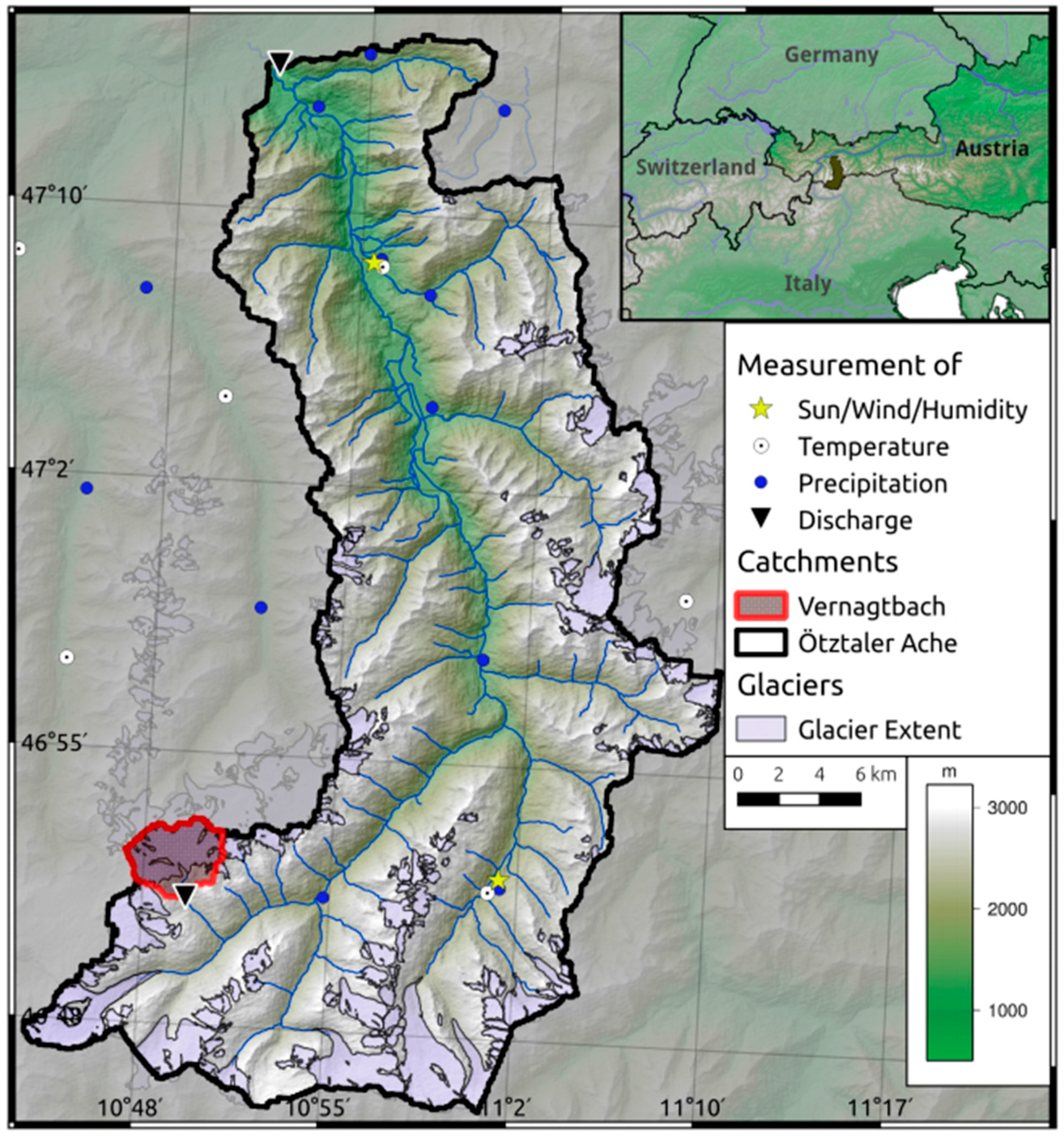
2. Study Site and Data

We studied the following two alpine catchments in western Austria: (1) The entire catchment of the Ötztaler Ache, one of the main tributaries of the River Inn; and (2) the nested Vernagtbach catchment, a highly glaciated sub-basin of the Ötztaler Ache. The Ötztaler Ache, located in North Tyrol and one of the main tributaries of the River Inn, includes some of the largest glaciers and highest mountain ranges in Austria. Roughly 50% of the catchment altitude exceeds 2230 m, with the highest point at 3748 m a.s.l. and the lowest point at 703 m a.s.l. (Figure 1). The catchment has a north-south extent of approx. 55 km, an east-west extent of approximately 18 km and a total size of 887 km². Due to hydropower production in the northeastern part of the Ötztal, the efficient total catchment size is reduced to 846 km². The main valley is rather narrow, with a north-south alignment and main expositions of east and west. In the lower catchment areas deep soils like podsols, cambisols and luvisols dominate, whereas shallow soils such as regosols and lithosols are found at higher altitudes. The Ötztal valley is mainly covered by meadows/alpine pastures, rocks and coniferous forests (see

Table 1. Main characteristics of the investigated catchments.

Gauging Station	Brunau	Vernagtbach
Gauged river	Ötztaler Ache	Vernagtbach
Minimum altitude (m a.s.l.)	706	2640
Mean altitude (m a.s.l.)	2230	3127
Maximum altitude (m a.s.l.)	3768	3535
Catchment area (km2)	847	11
Coniferous forest	17%	0%
Rock	27%	29%
Meadows/alpine pastures	41%	1%
Glacier	13%	69%

for a summary). Roughly 13% of the basin is still glaciated, and the timberline is located at 2300 m a.s.l. [25]. The climate of the Ötztaler Ache catchment is characterised by a mean annual temperature of 7.3 °C and 714 mm precipitation in Oetz (760 m a.s.l.) and 2.1 °C and 846 mm in Obergurgl (1938 m a.s.l.). See [14] for the mean annual cycles of temperature, snow depth and precipitation in the region surrounding the Ötztaler Ache catchment.

Ice melt and snowmelt play a fundamental role, hence runoff is highly variable throughout the yearly cycle (e.g., with average low flows below 1 mm/day in winter and average high flows of up to 10 mm/day in summer). We studied the Ötztaler Ache catchment down to the gauging station Brunau, located at the northernmost tip of the catchment. There are no streamflow measurements for Brunau before 1 January 1983, so the Brunau streamflow for 1 January 1975, to 31 December 1982, was calculated based on a linear relationship with Tumpen station data (the next gauge approximately 10 km upstream, derived from daily data 1983–2012; R² = 0.98). Catchment 2 (Vernagtbach) has been the subject of numerous studies for the Bavarian Academy of Sciences and Humanities, Commission for Geodesy and Glaciology, Munich (e.g., [1,26,27]). It is covered by Vernagt glacier over approximately 69% (in 2006) of its surface area, has a mean altitude of 3127 m a.s.l. and thus depicts a glacial runoff regime. Runoff at Vernagtbach is measured from May to October; during the rest of the year, there is hardly any discharge.

Over the annual cycle, discharge at the Vernagtbach catchment is highly variable with maxima in July and August, mostly caused by the strong glacial melt during this time of year (cf. Figure A1 in the Appendix). Runoff in the rising Q limb mostly originates from snowmelt. Snowmelt is strongest in June, same as melt of snow on ice, whereas firn melt is highest in July. At the Brunau catchment, snowmelt instead of ice melt is the highest discharge contributor. Snow contributions are also highest in June. However, July is the month with the highest discharge due to glacial melt. For a full overview of the monthly discharges and the single contributions for both study catchments, see Figure A1 and Figure A2 in the Appendix.

The Ötztaler Ache and the Vernagtbach are suitable study catchments in several ways: (1) There is outstanding data availability due to hydropower and academic research activities; (2) There were no major land use changes in the Ötztal during the study period; (3) The Ötztal spans glaciated high-altitude zones down to lower-altitude valley plains, so it is possible to study both hydrological conditions within the same region. The combination of the Ötztaler Ache catchment and that of Vernagtbach allows a more precise determination of the glacier parameters, in particular by cross-checking with glacial mass balances. Furthermore, an analysis of the changes in the Vernagtbach catchment is necessary to understand the trend causes in the headwater catchments, as these causes might be different from those in mostly lower-altitude catchments.

For the hydrological model input, we used daily precipitation (29 stations), temperature (12 stations), wind speed (3 stations), sunshine duration (internally converted to radiation, 3 stations) and relative humidity (3 stations) data from stations that were located inside or close to the catchment area and ranged between 610 m and 2640 m. The data was provided by Hydrographischer Dienst Tirol (Innsbruck), the Commission for Geodesy and Glaciology (Munich), AlpS GmbH (Innsbruck), Zentralanstalt für Meteorologie und Geodynamik (Vienna) and Tiroler Wasserkraft AG (Innsbruck). In addition to meteorological input data, several input grids were necessary to run WaSiM ETH: A digital elevation model (DEM) was modified so that the simulated rivers and sub-basins corresponded to the real ones. Further, we used land use and soil type maps, all provided by AlpS GmbH and based on [28].

Glacier extents based on the Austrian glacier inventories [29,30] were used as model input and for calibration purposes. The first glacier inventory of the Ötztal Alps (1969) was used as an initial condition of glacial cover for the pre-calibration period. The second (1997) and third (2006) inventories served as calibration criteria. Additionally, seasonal glacier mass balances measured by the Commission for Geodesy and Glaciology, Munich (provided by [31]) were included into the calibration, as they had proven to be helpful for obtaining better parameter sets in various studies [32,33]. Wintertime accumulation was observed via snow pits and snow depth measurements across the glacier, while summertime mass balances were measured via ablation stakes [1].

3. Methods

3.1. Hydrological Model Setup

We used the fully distributed, deterministic hydrological model system WaSiM ETH (Water Balance Simulation Model), which is frequently used in mesoscale catchments (e.g., Graeff et al. [34]). It is a well-known rainfall-runoff model, with a detailed physically-oriented description of a multitude of processes in the water cycle and is suitable for long-term water balance simulations in alpine regions [35]. The model was set up for the whole Ötztal catchment using a daily temporal resolution and a 100 m spatial resolution [36].

WaSiM ETH requires spatially distributed meteorological input data. Due to the strong altitudinal dependence of temperature and precipitation, we applied a constant lapse rate (which was included in the calibration process, see

Table 2. Most sensitive model parameters for both catchments with their estimated values.

Parameter	Value
Lapse rates
Temperature gradient (°C/m)	−0.006
Precipitation gradient (mm/m)	0.0024
Ice model
Degree-day-factor for ice (mm/°C/d)	7.9
Degree-day-factor for firn (mm/°C/d)	7.2
Degree-day-factor for snow on ice (mm/°C/d)	4.8
V-A-scaling (m)	29.8
V-A-exponent ( )	1.36
Snow model
Temperature limit for rain (°C)	1.5
Temperature limit for snow melt (°C)	0.9
Degree-day-factor for snow (mm/°C/d)	2.4
Transition zone for rain-snow (°C)	0.9
Soil model
Recession parameter (m)	0.04
Correction factor for transmissivities ( )	0.002

) combined with nearest neighbour. For wind speed, air humidity and sunshine duration, an inverse distance interpolation scheme was used. After interpolation of station data, temperature and radiation were adjusted internally to account for shadowing and exposition. To cope with the issue of gauge undercatch, we set a fixed precipitation correction factor of 7% more per m/s wind speed plus a 50% constant that is added to the daily precipitation observations in the case of snowfall. During rainfall, we did not apply any correction. The resulting total annual precipitation sums correspond to previous modelling studies in the area (e.g., [1]).

The dynamic glacier module is a new feature in WaSiM ETH, and allows changes in the glacier extent. With this, it is possible to calibrate the glacier model not only at discharges and glacier mass balances, but also at observed glacier extents. The procedure of glacial growth and shrinking is calculated via the volume-area scaling [37,38], an empirical relation, which is based on globally measured mass balances. Depending on the annual mass balance, glaciated cells are added or removed for each glacier iteratively once a year, in our case September 30 (i.e., only on this day of year, the model updates glacier extents). Furthermore, the module allows for partially glaciated cells, and the transformation of old snow into firn and finally into ice after a certain amount of time. This firn module is a substantial advantage of WaSiM ETH compared to other models. For more information on the dynamic glacier module, see [36].

Ice melt, firn melt and snowmelt were computed via the commonly used degree-day factor (DDF). During model calibration, the DDF proved to be more powerful in simulating melt processes than more sophisticated algorithms such as those after Anderson [39] or Hock [40], a fact that corresponds to other studies on a catchment scale [41]. To compute the soil water processes, we enabled the TOPMODEL approach [42] in WASIM ETH with an improved description of the macropore processes following Niehoff et al. [43], as it better suited the situation of available soil data and reduced computation times. Next to the above-mentioned modules, we also enabled the evapotranspiration, the infiltration and the interception modules.

As one of the aims of this paper was to fit modelled to simulated streamflow trends, a model period that was long enough to derive trends was necessary. We used the period 1980 to 2007 for calibration. For validation, we selected two shorter periods before and after the calibration period to consider temporal parameter instability (1975–1979 and 2008–2012, Figure 2). For all runs, we began simulations with spin-up periods (for calibration: 1969 to 1979; for the first validation period: 1969–1974; for the second: 1997–2007) to guarantee that all model storages (soil, snow, glacier, firn) were in equilibrium. If this was not the case after the spin-up period, we reran the model another time for the same spin-up period. With this temporal setup, it was possible to use the glacier inventory from 1969 as an initial condition and those from 1997 and 2006 for the calibration of the model.

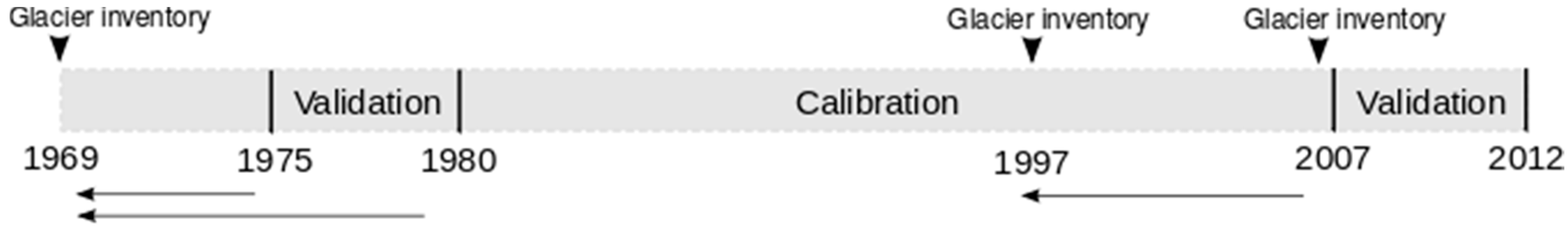
3.2. Calibration and Validation Scheme

To fit the hydrological model to the actual conditions, a multi-objective calibration approach based on several criteria was applied, considering the hydrograph, glacier extents, glacier mass balances, water balance terms and trends:

(1)

As recommended in Krause et al. [44], we derived several statistical measures to compare the simulated with the observed hydrograph, which included the Nash-Sutcliffe efficiency (NSE, [45]), the modified index of agreement (MD, [46]) and the coefficient of determination (R2). As the model efficiency is often overestimated by the standard Nash-Sutcliffe efficiency in time series with strong seasonality, the benchmark Nash-Sutcliffe coefficient based on a calendar-day model (NSE_bench, [47]) was also computed.

(2)

To consider glacier growth and shrinkage within the calibration process, we derived the following two measures calculated from simulated and observed extents of the Vernagt glacier: First, the “probability of detection” (POD) is the percentage of grid cells that were detected correctly (both in simulated and observed grids). Next, the “false alarm rate” (FAR) indicates the percentage of grid cells in the simulated glacier grid that were not found in the observed one [48]. Finally, the absolute simulated and observed glacier areas were compared.

(3)

As the glacier extents only gave information about the conditions at the beginning and end of the calibration period, we then used seasonal mass balances of the Vernagt glacier to calibrate the model. Thus, the temporal dynamic of ice melt and accumulation was also accounted for.

(4)

After this, discrepancies in the total simulated water budget were considered by comparing simulated average annual streamflow and average seasonal mass balances to the observed ones.

(5)

Most important for the goal of the present study was to fit the simulated trends to the observed trends during calibration. This was conducted for trends in annual streamflow, trends in glacier mass balances and, lastly, for highly resolved trends. This last point, the agreement of the simulated high-resolution trends with the observed trends, was the basis for the trend attribution attempt in the present analysis.

We applied a two-step calibration: First, the model was calibrated automatically, using the NSE_bench as the calibration criterion, to test the sensitivity of the model parameters, filter the most relevant ones and get an estimate of their ranges. We used the dynamically dimensioned search (DDS) optimization procedure [49] in a parallel implementation for the R environment (package ppso, [50]). DDS is a global, computationally effective and robust optimisation algorithm that requires no parameter tuning and is especially suitable for cases with many parameters to be calibrated. The parameter search is dynamically adjusted from a global to a more local scale via a reduction in parameter values in the neighbourhood, as the number of function calls approaches the user-specified maximum number of evaluations.

Afterwards, we fine-tuned model parameters manually in order to sufficiently satisfy the other calibration criteria. This manual calibration was conducted as a gradual process, similar to Stahl et al. [32]. First, the lapse rates of temperature and precipitation were calibrated such that the simulated corresponded with the observed glacial winter mass balances. Subsequently, we calibrated the snow and glacier parameters to achieve agreement of the streamflow goodness measures, summer mass balances, annual streamflow and glacial extents. Finally, we further fine-tuned the model parameters to reproduce the observed trends as exactly as possible. The soil parameters were not calibrated again, but were taken from the best parameter set during automatic calibration. Similar to all multi-objective calibration procedures, at a certain calibration step there is no increase in one goodness criterion without a decrease in another one. At the end of an extensive calibration procedure, we found a set of parameters which satisfied most calibration criteria adequately.

Most of the calibration criteria mentioned above were also used for the validation of the optimised model parameters found during calibration. For the objective functions (1) glacier area and (2) trends, proper validation was not possible due to (1) no glacier inventory during the validation period and (2) no sufficiently long validation period from which to derive trends.

3.3. Trend Detection

To understand the streamflow changes in the study catchments, we analysed trends based on averages of different temporal windows, i.e., annual averages to examine whether the interannual trends were simulated correctly and glacier summer and winter mass balances. Lastly, highly resolved trends were computed, as they had proven powerful in earlier attribution studies, using an approach taken from Kormann et al. [14]: To calculate highly resolved trends, a time series of a certain variable was first converted into a centered 30-day moving average (30DMA) time series, so that later a 30DMA series for each day of the year (DOY) and each year in the study period 1980–2007 was available (1 January 1980, 1 January 1981, … 1 January 2007; 2 January 1980, 2 January 1981, … 2 January 2007, etc.). Each of these 28-year series were subsequently analysed on trend magnitudes. This was based on the robust Sen’s Slope Estimator, which calculates the median of the slope between all possible pairs of data points [51]. The overall procedure resulted in a dataset that provided the 30DMA trend magnitude of a certain variable for each day of the year. The 30DMA trends were calculated for the observed and simulated hydrographs, providing an additional calibration criterion. After that, 30DMA trends of all major modelled runoff components (runoff from snowmelt, firnmelt, icemelt) and from interpolated temperature and evapotranspiration were computed.

We refrained from presenting the statistical significance of the detected trends in common with many newer studies that criticise the use of significance tests, such as the commonly used Mann-Kendall test [22,52]. Major issues with these tests include the potential violations of certain statistical assumptions next to problems of detectability [53]. For the main goal of this study (which is the attribution of trends), statements on significance are not important and might even hinder the detection of certain trend patterns.

3.4. Trend Attribution

Similar to Kormann et al. [9], we attributed the highly resolved trends by comparing trend magnitudes of different variables on certain days of the year with one another. If there were similar trend characteristics of streamflow and another variable during certain DOYs, we supposed that there was an interaction between these variables. For example, if streamflow trends showed a similar structure to the trends of forcing variables such as temperature, one could assume that the streamflow trends were caused directly or indirectly by the trends of these variables. Additionally, we added certain characteristic dates for both study catchments, taken from Kormann et al. [9], indicating when the long-term average minimum, maximum and mean temperatures cross the freezing point in spring and when the minimum temperature crosses it in autumn.

Following the scheme of Bronstert et al. [54] and the recommendations in Molnar et al. [5], we put the main focus of the attribution analysis on temperature-induced changes and how these changes affect streamflow. In the present study, we assume that a model, which is able to reproduce the overall observed streamflow trends, is also able to properly simulate the trends of the individual streamflow components. Hence, we examined trends in streamflow components such as ice melt, firn melt and snowmelt to analyse how the overall observed streamflow trend is composed.

Apart from trends in streamflow components, we also analysed trends in actual evapotranspiration, since ETa is expected to increase with global warming. This was conducted for the Brunau catchment only and not for the Vernagtbach sub-basin for the following reasons: (1) Evapotranspiration is generally a relatively small component of the total water balance of highly glaciated catchments—an estimated 120 mm/a in the Vernagtbach catchment, as reported in Braun et al. [1]; (2) Condensation happens more frequently than evaporation over snow- and ice-covered surfaces [1], and condensation is not included in WaSiM ETH. The same applies for sublimation, which can also be an important component of the moisture budget over snow and ice [55].

Further, we excluded precipitation in the attribution analysis, as the low signal-to-noise ratio allows no robust statements on detected changes and we found no clear trend in precipitation [14]. This also corresponds with other studies in the area (e.g., [56]).

4. Results

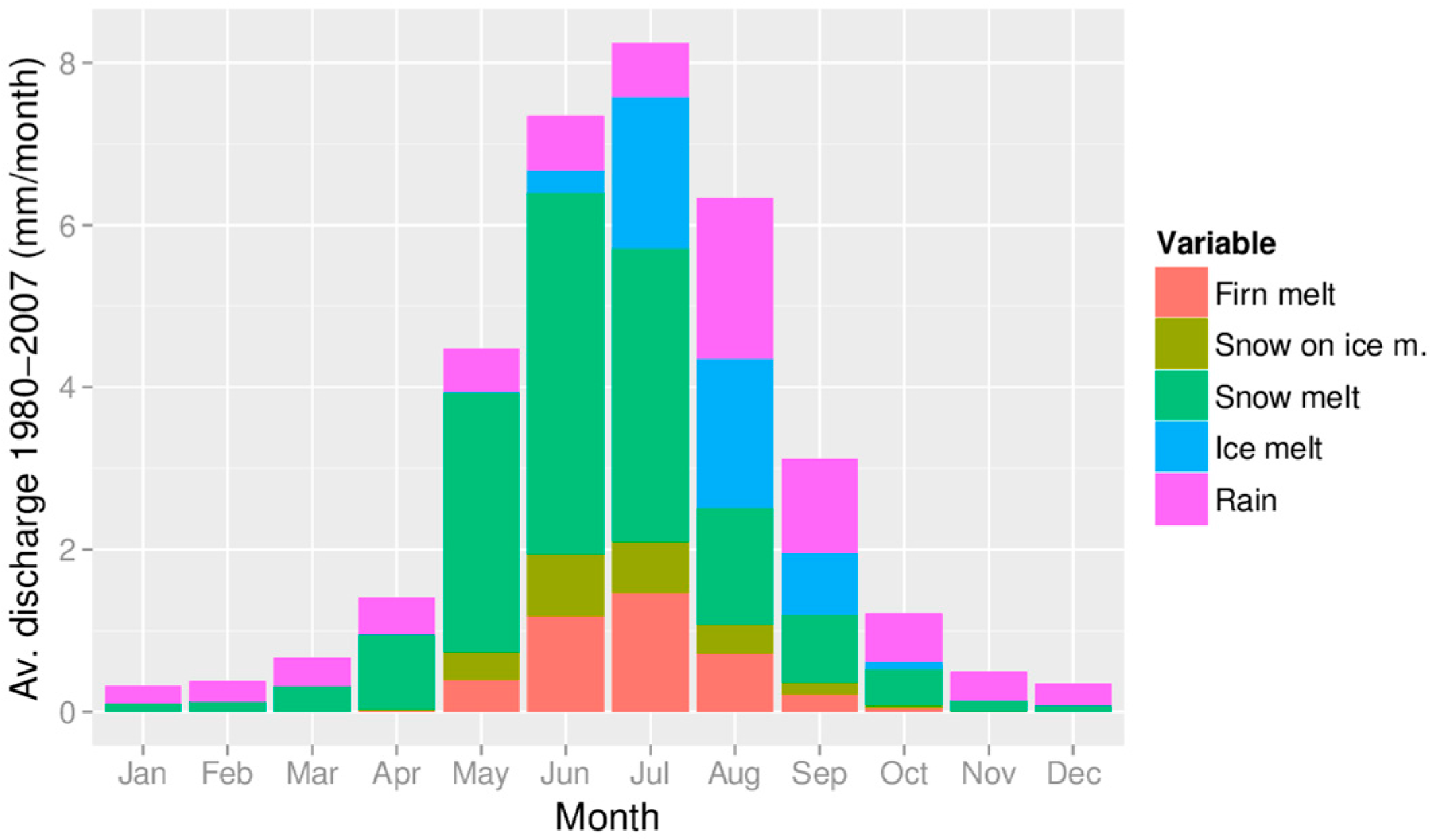
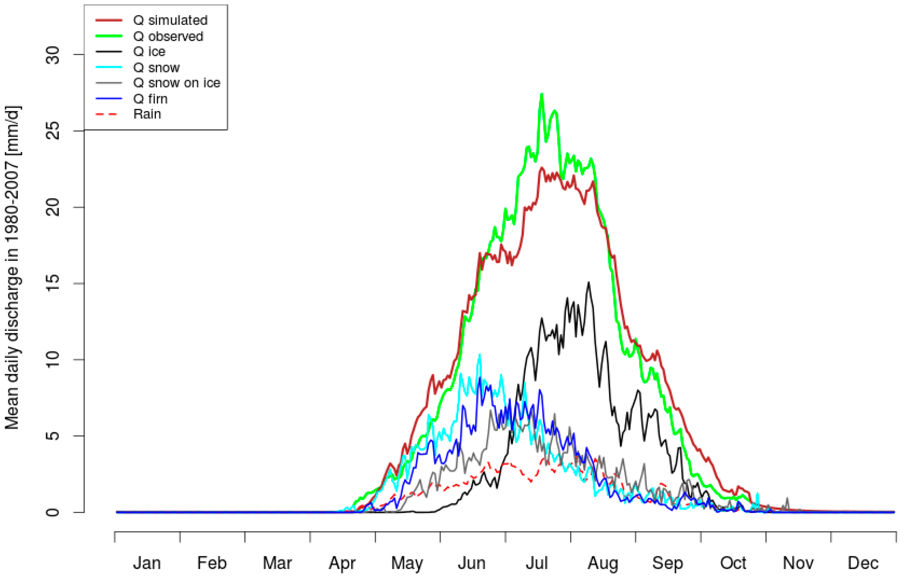
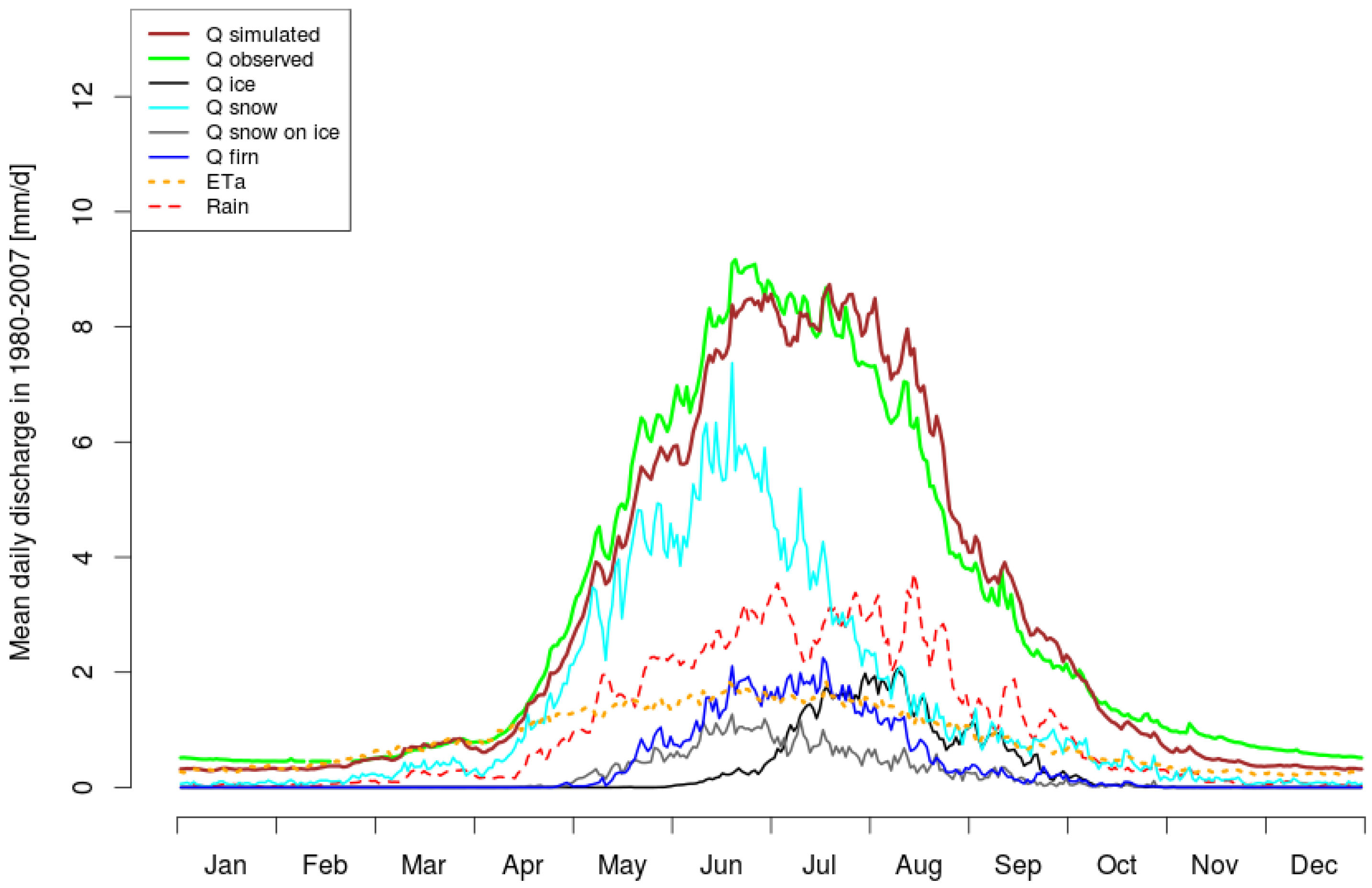
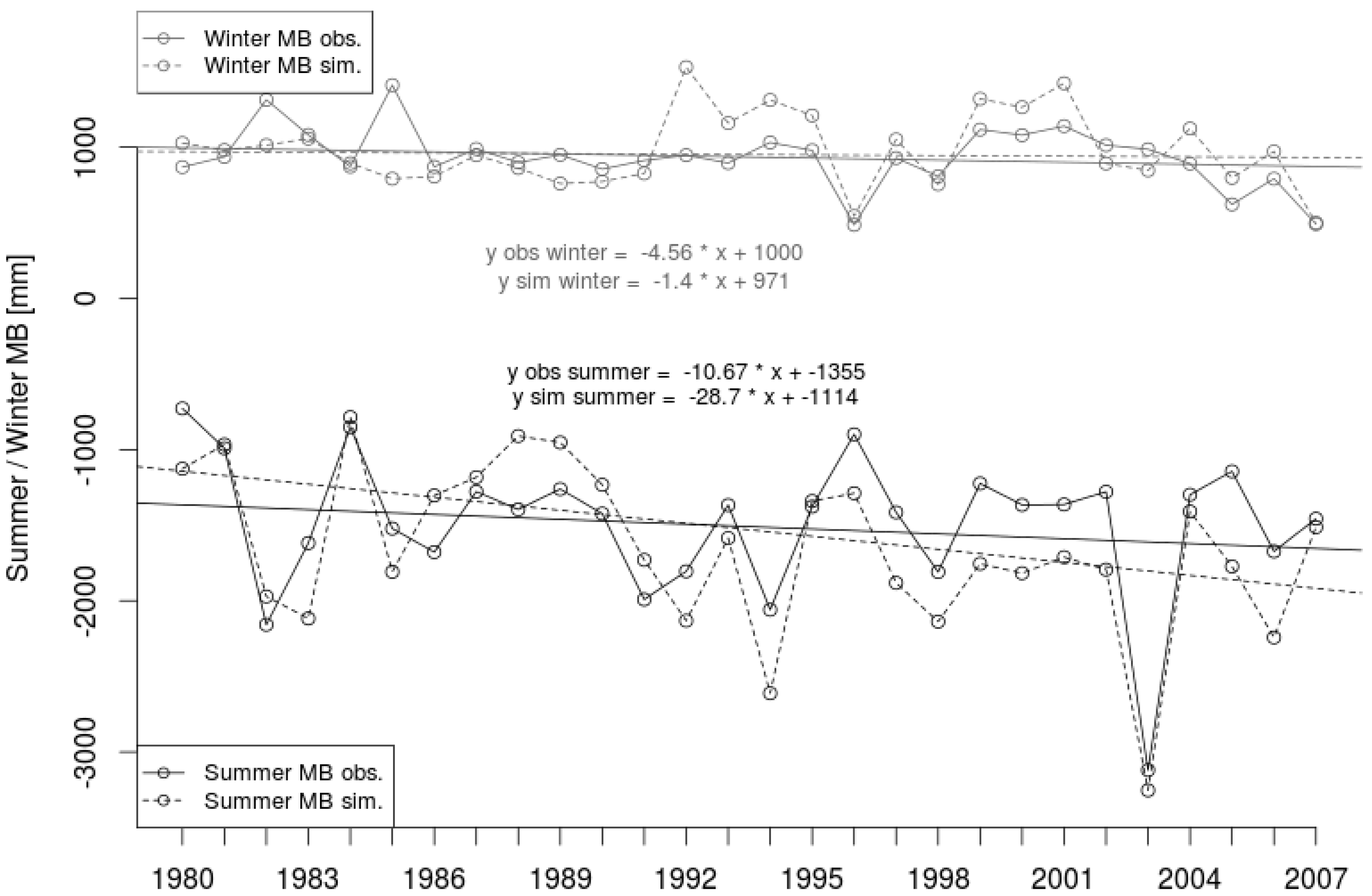
4.1. Calibration and Validation Results

During the pre-calibration sensitivity analysis we identified the most relevant model parameters that affect simulated streamflow. The majority of these parameters were related to ice melt, firn melt and snowmelt. Next to the temperature and precipitation lapse rates, the snow parameters (the threshold temperature rain/snow, the degree-day factor, the threshold temperature for snowmelt, and the temperature transition range from snow to rain) and the glacier parameters (the degree-day factor for ice, firn and snow on ice, and the VA-scaling and VA-exponent for the Volume-Area relation of glaciers) were highly sensitive. The soil parameters (especially the recession parameter and the correction factor for transmissivities) also influenced simulated streamflow, but to a lesser degree. After calibration, we obtained a set of parameters that simulates hydroclimatic conditions sufficiently well in both catchments (see Table 2 for an overview of the most relevant calibration parameters).

Standard goodness measures and mean annual hydrographs: The adequate agreement of both simulated and observed streamflow is reflected in the quality of the standard goodness measures (

Table 3. Model efficiency, simulated and observed annual streamflow and glacier mass balances for the calibration and validation periods (Q obs/sim = observed/simulated runoff; MB obs/sim = observed/simulated glacier mass balances).

	Calibration Period	Validation Periods
Vernagtbach	1980–2007	1975–1979	2008–2012
Nash-Sutcliffe efficiency *	0.82	0.74	0.81
R2 *	0.82	0.83	0.82
Index of agreement, mod. *	0.85	0.83	0.84
NS bench efficiency *	0.46	0.68	0.52
Mean annual Q obs (mm) *	1959	1179	2381
Mean annual Q sim (mm) *	1937	1419	2221
Mean summer MB obs (mm)	−1484	−750	−1751
Mean summer MB sim (mm)	−1654	−908	−1950
Mean winter MB obs (mm)	934	931	833
Mean winter MB sim (mm)	979	973	893
Brunau
Nash-Sutcliffe efficiency	0.91	0.91	0.87
R2	0.91	0.92	0.89
Index of agreement, mod.	0.89	0.88	0.88
NS bench efficiency	0.77	0.76	0.62
Mean annual Q obs (mm) *	1090	1011	1079
Mean annual Q sim (mm) *	1064	891	866

* calculated for May to October only

): During both calibration and validation, NSE, R2 and MD all show values around 0.8 for the Vernagtbach catchment, and those for Brunau even exceed those for Vernagtbach. The NSE_bench values that consider the seasonality of the time series range between 0.5 and 0.8.

Figure 3 demonstrates the ability of the model setup to simulate the seasonal mean daily hydrograph for the years 1980 to 2007 for the Vernagtbach catchment. The model performance was weaker in July, when simulated daily streamflow was approximately 3 to 4 mm/d lower than the observed value. The quantitatively most important streamflow components (in decreasing order) were runoff from ice melt, snowmelt and firn melt, with rainfall as the smallest streamflow contributor.

For the Brunau catchment, the model was able to simulate the mean daily streamflow with only small differences from the observed time series (Figure 4). The highest melt discharge contribution originated from the snow reservoir with liquid precipitation as the second highest contributor. Until June, snowmelt presented the only important contribution to streamflow. Minor contributors at this gauging station were melt from glaciers, firn and snow on glaciers (in decreasing order).

Glacier area and seasonal mass balances: Shrinkage and growth of glacier areas are generally simulated sufficiently well, which is shown by a high POD and a low FAR and a generally good agreement between simulated and observed glacier extents (

Table 4. Performance measures for observed vs. simulated extents for the Vernagt glacier (POD: probability of detection, FAR: false alarm rate).

	1997	2007
POD	0.93	0.9
FAR	0.02	0.04
Observed Extent (km2)	8.8	8.3
Simulated Extent (km2)	8.8	8

). Visually, deficiencies are mostly found in the inner structure of the glacier, where topographical features such as moraines affect the glacial melting behaviour (Figure 5). In these areas, the algorithm is not able to model the melting patterns sufficiently well, so that the modelled glacier appears rather smooth, whereas the observed one has several ice-free furrows.

Average annual streamflow and seasonal mass balances plus trends: After the above-mentioned calibration criteria, we evaluated both average annual streamflow and glacier mass balances for the period 1980 to 2007 plus their interannual variations and trends over time. Annual streamflow was simulated sufficiently well at both stations (Table 3) except that the simulated trend slope is lower than the observed one at Vernagtbach (Figure 6). While simulated winter glacier MBs were reproduced adequately, certain deficiencies exist in the modelled summer MBs, especially at the end of the time series (Figure 7).

30DMA trends: Daily streamflow trends were highly sensitive to changes in the relevant model parameters. Finding a good agreement between simulated and observed 30DMA trends was challenging due to the complexity of interactions between the several calibration objectives. However, the final set of parameters reproduced the overall trend structure well, especially at the Brunau gauging station. For the Vernagtbach gauging station, there were deviations between simulated and observed trend magnitudes in July and August, with simulated trends lower than the observed trends (Figure 8a and Figure 9a).

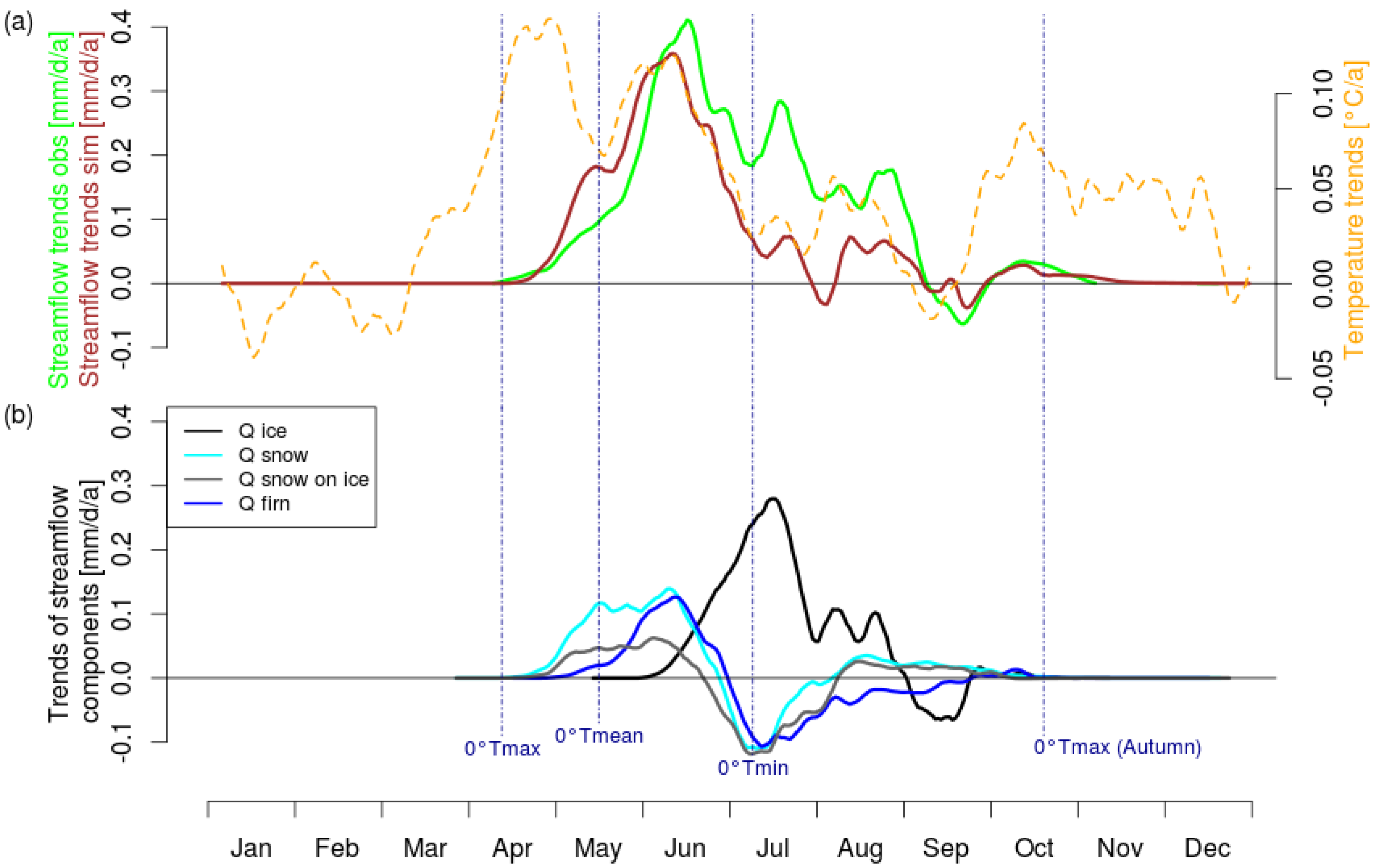
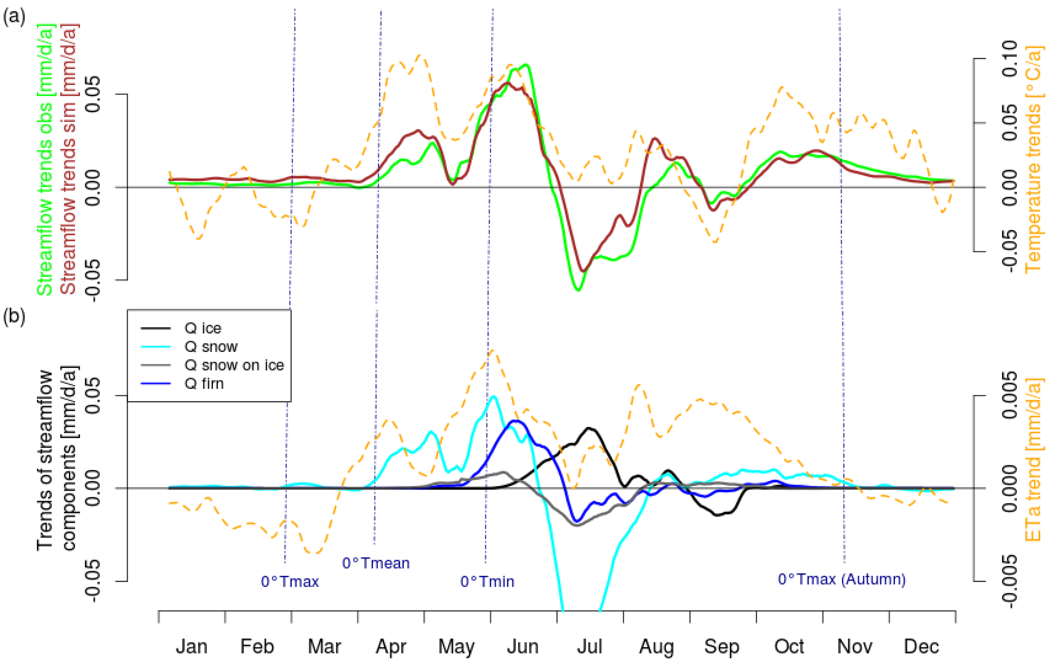
4.2. Attribution of Streamflow Trends

Vernagtbach (high-altitude catchment): There is considerable congruence of both simulated and observed streamflow trends with those of temperature throughout the runoff season (April—October, Figure 8a). During this time, streamflow trends seem to be coupled to the temperature trends with a delay of several days. This coupling starts roughly between the days when daily maximum and mean temperatures surpass the freezing point in spring and end shortly after the daily maximum temperature has crossed it in autumn. There are three corresponding peaks (mid-June, mid-July, and end of August) and one local minimum (September) in both simulated and observed streamflow trends. To some degree, these phenomena also appear in the temperature trends.

Concerning the changes in streamflow components, trends of snow and firn follow a distinct behaviour pattern of first increasing and later decreasing trends (Figure 8b). The snow, firn and snow-on-ice trends all roughly sum up to the total simulated streamflow trends until mid-June, adding up to the first trend peak in this month at the Vernagtbach gauging station. From mid-June onwards, the trend in glacial melt rises to its maximum in mid-July. This is also the time when negative trends in snow and firn are strongest, thus counterbalancing the positive ice melt trends. Finally, in September, negative ice melt trends occur shortly after temperature trends are also negative.

Ötztaler Ache (mostly lower-altitude catchment): Major streamflow trend patterns appear as soon as the average daily mean temperature crosses the freezing point in spring, which is roughly in early April. During April and June, two positive 30DMA trend patterns can be observed at the Brunau gauging station (Figure 9a). These two patterns are followed by negative trends in July. The patterns mainly resemble the snow trends (Figure 9b). However, the snow trends are far more negative (−0.09 mm/d/a) than the overall streamflow trends in July. During this month, negative snow- and firn-melt trends are compensated by increased glacial melt, which happens similarly in the Vernagtbach catchment. However, the ice-melt trends are less strong (maximum: 0.03 mm/d/a) than the ones at Vernagtbach (maximum: 0.3 mm/d/a), and thus the total streamflow trend is negative.

Also at the Brunau gauging station, there is a certain similarity of streamflow trends with the trends of temperature during the first half of the runoff season and at the end: The first two positive streamflow trend patterns in April and June turn up exactly when two positive temperature trend patterns occur. Later in September, negative streamflow trends follow negative temperature trends. Looking at the other streamflow components, a strong positive trend pattern of firn melt occurs in May and June and is followed by a slightly negative one in July.

Major evapotranspiration trends occur from mid-April to the end of October, the average runoff period and the period when the mean daily temperature is above zero. The ETa trends are positive most of the time, with three major peaks. These peaks show similar timings to the temperature trends during the first half of the year, hinting at the causes for the ETa trends. The magnitude of the ETa trends is only about one-tenth that of the streamflow trends. During the 28-year calibration period, annual evapotranspiration depicts an increase of about 11 mm, compared to 359 mm average annual ETa (Figure 10).

5. Discussion

5.1. Overall Model Skill

The quality of the model fit in terms of streamflow goodness measures is comparable to other studies in alpine catchments (cf. [27]). However, in these watersheds, one should particularly consider the benchmark NSE according to Schaefli and Gupta [47]. As the seasonality is removed, NSE_bench values are generally lower than standard NSE values. For both study catchments, NSE_bench values are acceptable, ranging from between 0.5 and 0.8 during validation. Also, annually averaged water balance components and seasonal mass balances were modelled in good agreement with the observed values, deviations between simulated and observed values during calibration and validation were mainly in the range of 5 to 10 percent. Our model further proved suitable for modelling the change in glacier extents, considering the uncertainties in the use of volume-area scaling [57].

There are several incidences where the model skill is poor, especially at the Vernagtbach watershed: For instance, the simulated mean daily hydrograph at Vernagtbach is roughly 10% to 15% lower than the observed one during July (Figure 3). These errors are probably a result of the simplified process representations in the hydrological model such as the static degree-day-factor. Literature sources suggest that a DDF value that increases over the ablation season might provide better modelling results [58] and also spatially variable DDFs are proposed [59]. However, the consideration of temporal and spatial DDF variability would add numerous additional degrees of freedom to the simulation. Also, errors in the processing of the observational data play a role: Rating curves are especially prone to errors in estimating high runoff values, which is the case during this time of year. In addition, measurement and interpolation of precipitation in alpine areas is highly uncertain [60].

5.2. Modelling Streamflow Trends

The main benefits of using highly resolved trends as calibration criteria in hydrological models are a more confined calibration and a lower degree of equifinality. Especially in hydrological modelling studies in glaciated catchments, an appropriate strategy is necessary to cope with the issue of equifinality, as glacier parameters add many additional degrees of freedom to the model. For instance, using an incorrect calibration, errors in snow accumulation or precipitation interpolation might be counterbalanced by errors in glacier melt [61]. When including seasonal glacier mass balances, glacier extents or glacier area changes, the modeller is able to constrain this uncertainty [62,63]. However, these data sets are rarely available, especially for longer periods. Including 30DMA trends into the calibration of hydrological models in glacially influenced catchments forces simulated streamflow to undergo the same transient changes as the observed time series. Due to the strong reaction of glacier runoff to climate change, this procedure is particularly suitable for catchments with significant glacier coverage.

However, adding annual and seasonal trends to the multi-objective calibration is challenging. Some of the calibration objectives were only modelled with a certain degree of deviation from the observed time series. Especially in relation to the annual and daily trends, there was always a trade-off between a more precise simulation of the trends and a deterioration in the standard goodness measures. With regard to this point, the overall model fit can be seen as sufficiently good; further, only one set of parameters for both catchments sufficed (the entire Ötztaler Ache catchment of 847 km² and the Vernagtbach catchment of 11 km²).

5.3. Model-Based Trend Attribution

Vernagtbach: At the Vernagtbach gauging station, the first (and overall highest) trend pattern in June is caused by several factors, all induced by higher temperatures during this period: (1) There is an earlier depletion of the snow reserves in spring, also caused by decreases in snowfall [14,26]. This shift is reflected by the trend sequence of first increasing (in June) and later decreasing trends (in July) of roughly similar overall magnitude. It concerns both the snow reserves on glaciers and those on other surfaces; (2) The Vernagt glacier has lost the major part of its firn body during recent decades [1], causing positive trends in firn melt in June. However, the annual sum of firn melt trends is negative. This means that the firn body of the Vernagt glacier has already decreased to such a degree that firn melt is no longer increasing with higher temperatures but is decreasing due to the reduction in volume; (3) Glacial firn bodies have a high reservoir effect [64], thus the Vernagt glacier has lost an important buffer of spring snowmelt water, resulting in additional rising runoff trends from snow on glaciers. The next trend pattern, roughly in July, is the result of positive ice melt trends caused by glacial retreat minus negative snow and firn trends. Especially for the two trend patterns mentioned above, the advantages of the model-based attribution compared to the data-based attribution are obvious: Kormann et al. [9] reported that trends in June are mainly caused from higher glacial melt. The model approach in the present study revealed that this is only partially true: Higher firn melt and snowmelt cause the trend pattern in June while the main ice melt occurs in July. However, this is counterbalanced by negative firn melt and snowmelt trends. The negative streamflow trends in September obviously result from lower ice melt volumes due to decreasing temperature trends, as already reported in the data-based attribution. The last positive trend pattern in October occurs during the same time period as rising temperature trends, so, on the one hand, increased melt plays a major role. On the other hand, during autumn, the firn body drains the previously stored water from precipitation and melt [64]. This drainage water decreases due to a retreating firn cover, thus reducing the trends from temperature-induced increased melt. Finally, overall streamflow trend magnitudes are small anyway at this time of year, as air temperatures are also close to the freezing point.

Brunau: At the Brunau gauging station, particularly the magnitudes of streamflow trend components, are different to those at Vernagtbach, and represent the trends observed in other lower-altitude catchments with a glacier component (cf. [9]). The first two trend patterns in April and June are mainly caused by earlier snowmelt volumes. The earlier depletion of the snow reservoir subsequently results in a negative streamflow trend pattern in July. For both snow and snow on glaciers, the annual trend sums are negative (snow: −0.33 mm/a; snow on ice: −0.21 mm/a), meaning that there is not only a shift to earlier melt timing, but also a slight decrease in melt volume. These trend patterns also correspond to those of the model experiment of Déry et al. [22], who generated patterns of both volume and timing decreases in spring snowmelt on the basis of synthetic hydrographs. The positive annual sum of firn melt trends (0.54 mm) documents the loss of glacial firn bodies in the entire Ötztal valley. Contrary to the Vernagt glacier, the remaining firn bodies in the catchment are still in the phase of increased runoff caused by reductions in volume. This obviously also applies for the ice reserves of the glaciers.

In general, model-based attribution of streamflow trends proved to be a powerful and straightforward method. However, one has to keep in mind that there might be periods where the total runoff signal might be simulated correctly, although the model underestimates the contributions from e.g., snow melt and overestimates the ones from ice melt. For this reason, also the trend signal of the single runoff component might be subject to errors. Including further calibration criteria such as glacial mass balances and glacier extents—as it was done in this study—restrains this issue, though.

5.4. The Role of Evapotranspiration

We found that ETa in our study region has been rising during recent decades, which corresponds to other analyses for the middle latitudes, such as e.g., Kramer et al. [65] or Douville et al. [15]. However, the magnitude of the ETa increases is still too small to also detect its effects on the total streamflow trend. This has similarly been found by Alaoui et al. [66] for a catchment in Switzerland via a comparison between past and projected future streamflow trends. For total runoff, trends caused by snowmelt, firn melt and ice melt play a far more decisive role than those caused by ETa increases, especially during the time period when the highest ETa trends also occur. For this reason, we were not able to uneqivocally link decreasing total streamflow trends with rising ETa trends.

6. Conclusions

Several recent studies suggest that trend analyses in hydrology should not only interpret the causes of detected changes, but also soundly analyse the drivers of the trends (i.e., attribute the trends). In the present study, we showed that a more robust and detailed understanding of trend causes can be obtained via the combined use of a hydrological model and high-resolution streamflow trends (i.e., trends computed for each day of the year) for the two case study catchments in the western Austrian Alps—a large, mostly lower-altitude catchment that includes extensive valley plains and a nested high-altitude, heavily glaciated headwater catchment. By analysing trends of single streamflow components and selected atmospheric drivers, we were able to provide an in-depth picture of the trend drivers and their share of the total trend throughout the calendar year: In the high-altitude, glaciated study catchment, earlier firn melt and snowmelt are causing the first increasing streamflow trends in springtime. During summertime, rising trends originating from ice melt have the major share of the total runoff trends, although these are lowered by decreasing snowmelt and firn melt trends. This summation of positive and negative trends of all single streamflow components is a major complication of all streamflow trend attribution studies. Process-oriented and distributed hydrological modelling is a powerful way to handle this issue and understand the underlying patterns. In the lower-altitude catchment, it is mostly changes in snowmelt runoff in terms of earlier timing and lower melt volumes that affect total streamflow. However, trend components caused by glacial melt also have a considerable influence in the lower catchment. We further showed that simulated evapotranspiration has been rising during the last few decades. The lowering effect of the ETa increase on total streamflow could not be identified unequivocally due to its low magnitude and the stronger counteracting effect of increasing trends caused by ice, firn and snow melt during this time of year. However, with projected temperature increases for future scenarios (cf. [67]), it is very likely that this link might soon be identifiable with higher certainty. Also, other potential trend causes related to climate change that were not included in the present model experiment (such as additional vegetation greening, higher treelines, degradation of permafrost, changed weather patterns, etc.) that might play a more significant role in the future.

In the present study, we clearly identified temperature as the main streamflow trend driver in the study catchments, having direct effects on ice melt, firn melt and snowmelt. Streamflow is not only directly determined by temperature through processes over short time scales, which is no novelty, just as streamflow also reflects temperature changes over longer time scales. However, in this study we further clarified the link between streamflow trends over daily and decadal time scales: Streamflow changes occur on a daily basis throughout the calendar year. If these deviations from the normal level are stronger on certain calendar days than others and occur more frequently on this day with the passing of time (decades), it is likely that these changes are part of a trend. This trend presents the transient change on a certain day of year. Finally, summing up the daily trend patterns over the entire calendar year results in the overall, annual trend value.

A suggestion for future research is the transfer of the presented model-based attribution approach to other study areas. Due to the underlying physical processes, we expect similar results as the ones obtained in this study for many catchments in alpine areas. Applying this approach in lowland catchments might be more challenging due to the following reasons: Climate-change driven streamflow trends in lowland basins are usually less strong than the trends in alpine catchments and, in addition, typical lowland catchments are also more anthropogenically influenced.

References

1. Braun, L.N.; Escher-Vetter, H.; Siebers, M.; Weber, M. Water balance of the highly glaciated Vernagt basin, Ötztal Alps. In Proceedings of the “Alpine Space—Man And Environment” Conference, Innsbruck, Austria, 28–29 September 2006.
2. Viviroli, D.; Archer, D.R.; Buytaert, W.; Fowler, H.J.; Greenwood, G.B.; Hamlet, A.F.; Huang, Y.; Koboltschnig, G.; Litaor, M.I.; López-Moreno, J.I.; et al. Climate change and mountain water resources: Overview and recommendations for research, management and policy. Hydrol. Earth Syst. Sci. 2011, 15, 471–504. [Google Scholar] [CrossRef] [Green Version]
3. Barnett, T.P.; Adam, J.C.; Lettenmaier, D.P. Potential impacts of a warming climate on water availability in snow-dominated regions. Nature 2005, 438, 303–309. [Google Scholar] [CrossRef] [PubMed]
4. Pellicciotti, F.; Bauder, A.; Parola, M. Effect of glaciers on streamflow trends in the Swiss Alps. Water Resour. Res. 2010. [Google Scholar] [CrossRef]
5. Molnar, P.; Burlando, P.; Pellicciotti, F. Streamflow Trends in Mountainous Regions, Encyclopedia of Snow, Ice and Glaciers; Springer: Berlin, Germany, 2011; pp. 1084–1089. [Google Scholar]
6. Cramer, W.; Yohe, G.W.; Auffhammer, M.; Huggel, C.; Molau, U.; Dias, M.A.F.D.; Solow, A.; Stone, D.A.; Tibig, L. Detection and attribution of observed impacts. In Climate Change 2014: Impacts, Adaptation, and Vulnerability. Part A: Global and Sectoral Aspects; Contribution of Working Group II to the Fifth Assessment Report of the Intergovernmental Panel on Climate Change; Field, C.B., Barros, V.R., Dokken, D.J., Mach, K.J., Mastrandrea, M.D., Bilir, T.E., Chatterjee, M., Ebi, K.L., Estrada, Y.O., Genova, R.C., et al., Eds.; Cambridge University Press: Cambridge, UK; New York, NY, USA, 2014; pp. 979–1037. [Google Scholar]
7. Merz, B.; Vorogushyn, S.; Uhlemann, S.; Delgado, J.; Hundecha, Y. HESS Opinions “More efforts and scientific rigour are needed to attribute trends in flood time series”. Hydrol. Earth Syst. Sci. 2012, 16, 1379–1387. [Google Scholar] [CrossRef]
8. Delgado, J.M.; Apel, H.; Merz, B. Flood trends and variability in the Mekong river. Hydrol. Earth Syst. Sci. 2010, 14, 407–418. [Google Scholar] [CrossRef]
9. Kormann, C.; Francke, T.; Renner, M.; Bronstert, A. Attribution of high resolution streamflow trends in Western Austria—An approach based on climate and discharge station data. Hydrol. Earth Syst. Sci. 2015, 19, 1225–1245. [Google Scholar] [CrossRef]
10. Blöschl, G.; Ardoin-Bardin, S.; Bonell, M.; Dorninger, M.; Goodrich, D.; Gutknecht, D.; Matamoros, D.; Merz, B.; Shand, P.; Szolgay, J. At what scales do climate variability and land cover change impact on flooding and low flows? Invited Commentary. Hydrol. Process. 2007, 21, 1241–1247. [Google Scholar] [CrossRef]
11. Mote, P.W.; Hamlet, A.F.; Clark, M.P.; Lettenmaier, D.P. Declining mountain snowpack in Western North America. Bull. Am. Meteorol. Soc. 2005, 86, 1–39. [Google Scholar] [CrossRef]
12. Hodgkins, G.A.; Dudley, R.W. Changes in the timing of winter—spring streamflows in eastern North America, 1913–2002. Geophys. Res. Lett. 2006. [Google Scholar] [CrossRef]
13. Knowles, N.; Dettinger, M.D.; Cayan, D.R. Trends in snowfall versus rainfall in the Western United States. J. Clim. 2006, 19, 4545–4559. [Google Scholar] [CrossRef]
14. Kormann, C.; Francke, T.; Bronstert, A. Detection of regional climate change effects on alpine hydrology by daily resolution trend analysis in Tyrol, Austria. J. Water Clim. Chang. 2015, 6, 124–143. [Google Scholar] [CrossRef]
15. Douville, H.; Ribes, A.; Decharme, B.; Alkama, R.; Sheffield, J. Anthropogenic influence on multidecadal changes in reconstructed global evapotranspiration. Nat. Clim. Chang. 2013, 3, 59–62. [Google Scholar] [CrossRef]
16. Stewart, I.; Cayan, D.; Dettinger, M. Changes toward earlier streamflow timing across western North America. J. Clim. 2005, 18, 1136–1155. [Google Scholar] [CrossRef]
17. Birsan, M.V.; Molnar, P.; Pfaundler, M.; Burlando, P. Streamflow trends in Switzerland. J. Hydrol. 2005, 314, 312–329. [Google Scholar] [CrossRef]
18. Stahl, K.; Moore, R.D. Influence of watershed glacier coverage on summer streamflow in British Columbia, Canada. Water Resour. Res. 2006. [Google Scholar] [CrossRef]
19. Hidalgo, H.G.; Das, T.; Dettinger, M.D.; Cayan, D.R.; Pierce, D.W.; Barnett, T.P.; Bala, G.; Mirin, A.; Wood, A.W.; Bonfils, C.; et al. Detection and Attribution of Streamflow Timing Changes to Climate Change in the Western United States. J. Clim. 2009, 22, 3838–3855. [Google Scholar] [CrossRef]
20. Hamlet, A.F.; Mote, P.W.; Clark, M.P.; Lettenmaier, D.P. Twentieth-century trends in runoff, evapotranspiration, and soil moisture in the western United States. J. Clim. 2007, 20, 1468–1486. [Google Scholar] [CrossRef]
21. Maurer, E.P.; Stewart, I.T.; Bonfils, C.; Duffy, P.B.; Cayan, D. Detection, attribution, and sensitivity of trends toward earlier streamflow in the Sierra Nevada. J. Geophys. Res. Atmos. 2007, 112, 1984–2012. [Google Scholar] [CrossRef]
22. Duethmann, D.; Bolch, T.; Farinotti, D.; Kriegel, D.; Vorogushyn, S.; Merz, B.; Pieczonka, T.; Jiang, T.; Su, B.; Güntner, A. Attribution of streamflow trends in snow and glacier melt dominated catchments of the Tarim River, Central Asia. Water Resour. Res. 2015, 51, 1944–7973. [Google Scholar] [CrossRef]
23. Déry, S.J.; Stahl, K.; Moore, R.D.; Whitfield, P.H.; Menounos, B.; Burford, J.E. Detection of runoff timing changes in pluvial, nival, and glacial rivers of western Canada. Water Resour. Res. 2009. [Google Scholar] [CrossRef]
24. Kim, J.-S.; Jain, S. High-resolution streamflow trend analysis applicable to annual decision calendars: A western United States case study. Clim. Chang. 2010, 102, 699–707. [Google Scholar] [CrossRef]
25. Patzelt, G. Das Ötztal—Topographische Kennzeichnung. In Glaziale und Periglaziale Lebensräume im Raum Obergurgl; Koch, E.M., Erschbamer, B., Eds.; Innsbruck University Press: Innsbruck, Austria, 2010; pp. 9–11. [Google Scholar]
26. Braun, L.; Weber, M.; Mauser, W.; Prasch, M. Hydrometeorological Monitoring of Vernagtferner as an Essential Basis for Snow and Glacier Modelling in the GLOWA-Danube Project. The Application of Observations and Models for Assessing Water Resources and Risks in Mountain Areas, with the Related Uncertainties; Société Hydrotechnique de France (SHF): Paris, France, 2011; pp. 207–221. [Google Scholar]
27. Mayr, E.; Hagg, W.; Mayer, C.; Braun, L. Calibrating a spatially distributed conceptual hydrological model using runoff, annual mass balance and winter mass balance. J. Hydrol. 2013, 478, 40–49. [Google Scholar] [CrossRef]
28. Austrian Federal Ministry of Agriculture, Forestry, Environment and Water Management (BMLFUW). Hydrologischer Atlas Österreichs; BMLFUW: Vienna, Austria, 2007.
29. Kuhn, M.; Lambrecht, A.; Abermann, J. Austrian Glacier Inventory 1998. Available online: http://doi.pangaea.de/10.1594/PANGAEA.809196 (accessed on 16 February 2015).
30. Abermann, J.; Seiser, B.; Meran, I.; Stocker-Waldhuber, M.; Goller, M.; Fischer, A. The Third Glacier Inventory of North Tyrol, Austria, for 2006. Available online: http://doi.pangaea.de/10.1594/PANGAEA.806960 (accessed on 16 February 2015).
31. Zemp, M.; Nussbaumer, S.U.; Naegeli, K.; Gärtner-Roer, I.; Paul, F.; Hoelzle, M.; Haeberli, W. WGMS Glacier Mass Balance Bulletin No. 12 (2010–2011); ICSU(WDS)/IUGG(IACS)/UNEP/UNESCO/WMO, World Glacier Monitoring Service: Zurich, Switzerland, 2013; p. 106. [Google Scholar]
32. Stahl, K.; Moore, R.D.; Shea, J.M.; Hutchinson, D.; Cannon, A.J. Coupled modelling of glacier and streamflow response to future climate scenarios. Water Resour. Res. 2008. [Google Scholar] [CrossRef]
33. Schaefli, B.; Huss, M. Integrating point glacier mass balance observations into hydrologic model identification. Hydrol. Earth Syst. Sci. 2011, 15, 1227–1241. [Google Scholar] [CrossRef]
34. Graeff, T.; Zehe, E.; Blume, T.; Francke, T.; Schröder, B. Predicting event response in a nested catchment with generalized linear models and a distributed watershed model. Hydrol. Process. 2012, 26, 3749–3769. [Google Scholar] [CrossRef]
35. Jasper, K.; Calanca, P.; Gyalistras, D.; Fuhrer, J. Differential impacts of climate change on the hydrology of two alpine river basins. Clim. Res. 2004, 26, 113–129. [Google Scholar] [CrossRef]
36. Schulla, J. Model Description WaSiM (Water Balance Simulation Model). Available online: http://www.wasim.ch/downloads/doku/wasim/wasim_2013_en.pdf (accessed on 30 July 2015).
37. Chen, J.; Ohmura, A. Estimation of Alpine Glacier Water Resources and Their Change Since the 1870s; IAHS Publ.: Wallingford, UK, 1990; pp. 127–135. [Google Scholar]
38. Bahr, D.B.; Meier, M.F.; Peckham, S.D. The physical basis of glacier volume-area scaling. J. Geophys. Res. 1997, 102, 20–355. [Google Scholar] [CrossRef]
39. Anderson, E.A. National Weather Service River Forecast System—Snow Accumulation and Ablation Model; Tech. Mem., NWS-HYDRO-17; National Oceanographic and Atmospheric Administration (NOAA), U.S. Department of Commerce: Washington, DC, UK, 1973; p. 217.
40. Hock, R. Modeling of Glacier Melt and Discharge. Ph.D. Thesis, Verlag Geographisches Institut ETH Zürich, Zürich, Netherlands, 1998; p. 140. [Google Scholar]
41. Hock, R. Temperature index melt modelling in mountain areas. J. Hydrol. 2003, 282, 104–115. [Google Scholar] [CrossRef]
42. Beven, K.J.; Kirkby, M.J. A physically based variable contributing area model of basin hydrology. Hydrol. Sci. Bull. 1979, 24, 43–69. [Google Scholar] [CrossRef]
43. Niehoff, D.; Fritsch, U.; Bronstert, A. Land-use impacts on storm-runoff generation: Scenarios of land-use change and simulation of hydrological response in a meso-scale catchment in SW-Germany. J. Hydrol. 2000, 267, 80–93. [Google Scholar] [CrossRef]
44. Krause, P.; Boyle, D.P.; Bäse, F. Comparison of different efficiency criteria for hydrological model assessment. Adv. Geosci. 2005, 5, 89–97. [Google Scholar] [CrossRef]
45. Nash, J.; Sutcliffe, J. River flow forecasting through conceptual models (1), a discussion of principles. J. Hydrol. 1970, 10, 282–290. [Google Scholar] [CrossRef]
46. Zambrano-Bigiarini, M. HydroGOF: Goodness-of-Fit Functions for Comparison of Simulated and Observed Hydrological Time Series. R Package Version 0.3–8. 2014. Available online: http://www.rforge.net/hydroGOF/ (accessed on 20 January 2015).
47. Schaefli, B.; Gupta, H. Do Nash values have value? Hydrol. Process. 2007, 21, 2075–2080. [Google Scholar] [CrossRef]
48. Murphy, A.; Winkler, R. A general framework for forecast verification. Mon. Weather Rev. 1986, 119, 1330–1338. [Google Scholar] [CrossRef]
49. Tolson, B.A; Shoemaker, C.A. Dynamically dimensioned search algorithm for computationally efficient watershed model calibration. Water Resour. Res. 2007. [Google Scholar] [CrossRef]
50. Francke, T. Particle Swarm Optimization and Dynamically Dimensioned Search, Optionally Using Parallel Computing Based on Rmpi. R Package Version 0.9–989. 2014. Available online: https://www.rforge.net/doc/packages/ppso/00Index.html (accessed on 20 February 2015).
51. Helsel, D.R.; Hirsch, R.M. Statistical Methods in Water Resources; Elsevier Science: Amsterdam, the Netherlands, 1992. [Google Scholar]
52. Stahl, K.; Tallaksen, L.M.; Hannaford, J.; van Lanen, H.A.J. Filling the white space on maps of European runoff trends: Estimates from a multi-model ensemble. Hydrol. Earth Syst. Sci. 2012, 16, 2035–2047. [Google Scholar] [CrossRef] [Green Version]
53. Morin, E. To know what we cannot know: Global mapping of minimal detectable absolute trends in annual precipitation. Water Resour. Res. 2011. [Google Scholar] [CrossRef]
54. Bronstert, A.; Kolokotronis, V.; Schwandt, D.; Straub, H. Comparison and Evaluation of regional climate scenarios for hydrological impact analysis: General scheme and application example. Int. J. Clim. 2007, 27, 1579–1594. [Google Scholar] [CrossRef]
55. Strasser, U.; Bernhardt, M.; Weber, M.; Liston, G.E.; Mauser, W. Is snow sublimation important in the alpine water balance? Cryosphere 2008, 2, 53–66. [Google Scholar] [CrossRef]
56. Schimon, W.; Schöner, W.; Böhm, R.; Haslinger, K.; Blöschl, G.; Merz, R.; Blaschke, A.P.; Viglione, A.; Parajka, J.; Kroiß, H.; et al. Anpassungsstrategien an den Klimawandel für Österreichs Wasserwirtschaft; Bundesministerium für Land und Forstwirtschaft, Umwelt und Wasserwirtschaft: Vienna, Austria, 2011. [Google Scholar]
57. Radić, V.; Hock, R.; Oerlemans, J. Volume–area scaling vs. flowline modelling in glacier volume projections. Ann. Glaciol. 2007, 46, 234–240. [Google Scholar] [CrossRef]
58. DeWalle, D.R.; Henderson, Z.; Rango, A. Spatial and temporal variations in snowmelt degree-day factors computed from SNOTEL data in the Upper Rio Grande basin. In Proceedings of the Western Snow Conference, Granby, CO, USA, 20 May 2002; p. 73.
59. Bormann, K.J.; Evans, J.P.; McCabe, M.F. Constraining snowmelt in a temperature-index model using simulated snow densities. J. Hydrol. 2014, 517, 652–667. [Google Scholar] [CrossRef]
60. Blumer, F. Altitudinal Dependence of Precipitation in the Alps. Ph.D. Thesis, ETH Zürich, Zürich, Switzerland, 1994. [Google Scholar]
61. Jost, G.; Moore, R.D.; Menounos, B.; Wheate, R. Quantifying the contribution of glacier runoff to streamflow in the upper Columbia River Basin, Canada. Hydrol. Earth Syst. Sci. 2012, 16, 849–860. [Google Scholar] [CrossRef] [Green Version]
62. Schaefli, B.; Hingray, B.; Niggli, M.; Musy, A. A conceptual glacio-hydrological model for high mountainous catchments. Hydrol. Earth Syst. Sci. 2005, 9, 95–109. [Google Scholar] [CrossRef]
63. Konz, M.; Seibert, J. On the value of glacier mass balances for hydrological model calibration. J. Hydrol. 2010, 385, 238–246. [Google Scholar] [CrossRef] [Green Version]
64. Fountain, A.G. Effect of snow and firn hydrology on the physical and chemical characteristics of glacial runoff. Hydrol. Process. 1996, 10, 509–521. [Google Scholar] [CrossRef]
65. Kramer, R.J.; Bounoua, L.; Zhang, P.; Wolfe, R.E.; Huntington, T.G.; Imhoff, M.L.; Thome, K.; Noyce, G.L. Evapotranspiration trends over the eastern United States during the 20th century. Hydrology 2015, 2, 93–111. [Google Scholar] [CrossRef]
66. Alaoui, A.; Willimann, E.; Jasper, K.; Felder, G.; Herger, F.; Magnusson, J.; Weingartner, R. Modelling the effects of land use and climate changes on hydrology in the Ursern valley, Switzerland. Hydrol. Process. 2014, 28, 3602–3614. [Google Scholar] [CrossRef]
67. Tecklenburg, C.; Francke, T.; Kormann, C.; Bronstert, A. Modeling of water balance response to an extreme future scenario in the Ötztal catchment, Austria. Adv. Geosci. 2012, 32, 63–68. [Google Scholar] [CrossRef]
Figure 1. Map of the study area with location of the gauging stations, catchment boundaries, glacier coverage and closest meteorological stations.
Hydrology 03 00007 g001
Figure 2. Time bar to illustrate periods of calibration and validation, date of glacier inventories, and spin-up periods (arrows below).
Hydrology 03 00007 g002
Figure 3. Mean daily simulated and observed streamflow for the Vernagtbach catchment during the period 1980–2007 and its most important simulated components.
Hydrology 03 00007 g003
Figure 4. Mean daily simulated and observed streamflow for the Brunau catchment during the period 1980–2007, its most important simulated components and simulated ETa.
Hydrology 03 00007 g004
Figure 5. Observed (a,b) and simulated (c,d) extent of the Vernagt glacier for 1997 and 2007. Yellow coloured cells are entirely glaciated, orange to red ones are only partially glaciated.
Hydrology 03 00007 g005
Figure 6. Simulated and observed annual streamflow (Q) for Vernagtbach and Brunau gauging stations during the calibration period and linear trends (y obs/sim = observed/simulated runoff; x = year—1979).
Hydrology 03 00007 g006
Figure 7. Simulated and observed summer and winter glacier mass balances (MB) of Vernagt glacier during the calibration period and linear trends (y obs/sim = observed/simulated mass balance; x = year—1979).
Hydrology 03 00007 g007
Figure 8. (a) Daily trends of observed and simulated streamflow along with temperature trends at the Vernagtbach catchment (1980–2007); (b) Daily trends of the most important simulated streamflow components (1980–2007).
Hydrology 03 00007 g008
Figure 9. (a) Daily trends of observed and simulated streamflow along with temperature trends at the Brunau catchment (1980–2007); (b) Daily trends of the most important simulated streamflow components along with ETa trends (1980–2007). Please note the different scaling of the axes of streamflow component trends and ETa trends in (b).
Hydrology 03 00007 g009
Figure 10. Simulated annual evapotranspiration (ETa) for the Brunau catchment, plus linear trend (y sim = simulated ETa; x = year—1979).
Hydrology 03 00007 g010