Article

Evapotranspiration Trends Over the Eastern United States During the 20th Century

1
Rosenstiel School of Marine and Atmospheric Science, University of Miami, 4600 Rickenbacker Causeway, Miami, FL 33149, USA
2
Biospheric Sciences Laboratory, Code 618, NASA Goddard Space Flight Center, NASA Goddard Space Flight Center, Code 618, Greenbelt, MD 20771, USA
3
Earth System Science Interdisciplinary Center, University of Maryland, College Park, MD 20742, USA
4
Terrestrial Information Systems Research, Code 619, NASA Goddard Space Flight Center, NASA Goddard Space Flight Center, Code 619, Greenbelt, MD 20771, USA
5
Maine Water Science Center, U.S. Geological Survey, 196 Whitten Road, Augusta, ME 04330, USA
6
Joint Global Change Research Institute, Pacific Northwest National Laboratory, 2825 University Research Court, Suite 1200, College Park, MD 20740, USA
7
Department of Geography, University of Toronto, 100 St. George Street, Toronto, ON M5S 3G3, Canada
*
Authors to whom correspondence should be addressed.
Hydrology 2015, 2(2), 93-111; https://doi.org/10.3390/hydrology2020093
Submission received: 11 November 2014 / Accepted: 4 May 2015 / Published: 14 May 2015

Abstract

:
Most models evaluated by the Intergovernmental Panel for Climate change estimate projected increases in temperature and precipitation with rising atmospheric CO2 levels. Researchers have suggested that increases in CO2 and associated increases in temperature and precipitation may stimulate vegetation growth and increase evapotranspiration (ET), which acts as a cooling mechanism, and on a global scale, may slow the climate-warming trend. This hypothesis has been modeled under increased CO2 conditions with models of different vegetation-climate dynamics. The significance of this vegetation negative feedback, however, has varied between models. Here we conduct a century-scale observational analysis of the Eastern US water balance to determine historical evapotranspiration trends and whether vegetation greening has affected these trends. We show that precipitation has increased significantly over the twentieth century while runoff has not. We also show that ET has increased and vegetation growth is partially responsible.

1. Introduction

The IPCC Fifth Assessment Report states that precipitation has generally increased over land in the Northern Hemisphere mid-latitudes [1]. Furthermore, there is substantial evidence to suggest that the hydrologic cycle has been intensifying with climate change [2,3,4]. These trends raise some questions. How is this hydrologic intensification being distributed across the cycle? To which components of the cycle has the additional precipitation been directed? What are the implications of these changes for the climate?
Some researchers suggest that the additional water available from increasing precipitation may stimulate an increase in vegetation growth and subsequently lead to an increase in evapotranspiration (ET) [5,6,7]. This process may induce a negative feedback on the climate, providing an additional cooling mechanism that may reduce the magnitude of the climate-warming trend.
Natural ET is comprised of canopy transpiration, interception loss (potential evaporation of precipitation intercepted by leaves on the canopy), and ground evaporation. The canopy-dependent component of ET responds to changes in vegetation structure [8,9,10], so that vegetation greening leads to an increase in ET, and to changes in atmospheric CO2 concentration and environmental stresses through stomatal adjustment [11,12]. Stressed vegetation tends to reduce its stomatal conductance and transpiration (e.g., [13]), leading to a warming effect, whereas unstressed vegetation facilitates the diffusion of water out of the plant during photosynthesis, and thus increases transpiration and cooling (e.g., [6]). ET can also be dictated in part by vapor pressure deficit (VPD) [14], defined as the saturation vapor pressure minus actual vapor pressure.
The authors of [15] analyzed trends in the components of the hydrological cycle in 19 climate models simulating the effects of an increase in CO2.The ensemble mean from these models indicates that, compared to their respective baselines over land, the global mean of runoff change would increase twice as fast as that of the precipitation. However, only a few of these simulations have considered the effects of vegetation-climate interactions. Conversely, the studies of [5,6,7] considered vegetation-climate interactions within climate models of different degrees of complexity in an environment with increased atmospheric CO2 concentration, and all three studies accounted explicitly for an increase in vegetation structure through increase in vegetation Leaf Area Index (LAI). Additionally, the authors of [6] introduced plant physiological down-regulation—a process by which plants reduce their photosynthetic activity under abundant atmospheric CO2. Under elevated CO2, plants exhibit some down-regulation characterized by a reduction in the initial CO2 enhanced rates of photosynthesis that result from a gradual decrease in the activity and/or amount of Rubisco, the enzyme in plant cells responsible for the first step in carbon fixation [16]. Down-regulation reduces the canopy conductance beyond the reduction caused by the radiative and physiological effects of increased CO2 [12], leading thus to increased water availability, which is diverted, as an additional effect, to increase LAI beyond increases caused by climate changes and CO2-induced water use efficiency. Each study compared the effects of the vegetation feedback on climate to a conventional simulation where vegetation structure was not allowed to change.
Results from all three simulations [5,6,7] suggested that an increase in vegetation density, or vegetation greening, will cause ET to increase. However, there was disagreement on the quantified significance of this potentially important feedback process and its global impact on the climate. In contrast to the models used in the analysis in [15], the study in [6] found the rate of change of precipitation to increase more than that of runoff. Furthermore, the authors of [5,6] simulated a reduction of warming trends associated with the increase in LAI and the authors of [7] found no significant global effect on climate.
While the modeling community has started to include the effect of this vegetation feedback on climate and assess its implications, the purpose of this study is to evaluate its significance by establishing an observational basis to determine whether ET has historically increased and whether an increase in ET may be related to an increase in vegetation.
Recognizing the difficulties in closing the water budget at regional or continental scales, and the lack of appropriate spatial data, our objective was to use available data to estimate the components of the hydrological cycle in order to analyze the historical evolution of ET over a large region of the eastern United States since the beginning of the twentieth century. We assess the trend in ET as a residual from the components of the water budget, including human water consumption, and compare it to changes in vegetation greening as inferred from the Normalized Difference Vegetation Index (NDVI).

2. Materials and Methods

2.1. Basin-Scale Water Budget
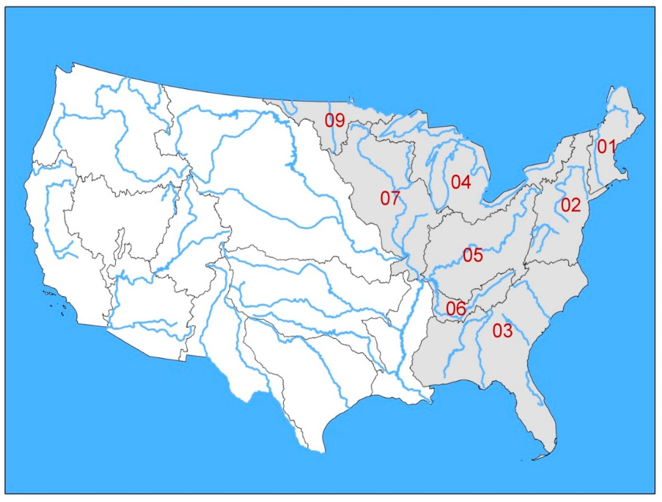
Over a contained hydrological basin where continuity equations apply, the natural (non-anthropogenic) water budget can be described by Equation (1) [17,18]:
P-Ru = ET + dS/dt(sw) + dS/dt(uz) + dS/dt(gw)
where P is the precipitation influx, Ru is the streamflow runoff, comprised of surface and groundwater runoff, and their difference (P-Ru) is partitioned into evapotranspiration (ET), change in surface water storage dS/dt(sw), change in moisture storage in the unsaturated zone dS/dt(uz) and change in storage of groundwater dS/dt(gw), respectively. At decadal to longer time scales and over hydrological units undisturbed by anthropogenic activities, an increasing trend in (P-Ru) must therefore be balanced by the net difference of evapotranspiration and storage trends. Over such long timescales many studies have shown that changes in surface water storage, dS/dt(sw), and storage in unsaturated zone, dS/dt(uz), are negligible (e.g., [19,20]).
Anthropogenic water use is increasing with increases in population and with increasing agricultural and industrial development. Water use is usually defined and measured in terms of withdrawal and consumption. Withdrawal refers to water extracted from surface or groundwater sources, and consumption refers to the part of a withdrawal that is ultimately used and removed from the hydrological unit, whether by evaporation, transpiration or incorporation into crops or other products. Conversely, the return flow is the portion of a withdrawal that is not actually consumed, and is instead returned to the hydrological unit [21]. Water consumption has been shown to have a non-negligible effect on the hydrological cycle at basin scales [22]. However, consumption data are not available at the basin scale over our study area. Therefore, we analyze precipitation, runoff and groundwater storage at the basin scale to evaluate the inter-basin variation, but only assess the trend in ET as a residual of the components of the water budget, including human water consumption, over the entire eastern United States study area, where anthropogenic water use statistics are available.

2.2. Study Area

Our study area covers 8 large hydrological units (New England, Mid Atlantic, South Atlantic-Gulf, Great Lakes, Ohio, Tennessee, Upper Mississippi, and Souris-Red-Rainy) that include the area east of the Mississippi River (Figure 1).
Figure 1. Eighteen major hydrological units as defined by the USGS encompass the continental US and are outlined with grey lines. The study area is shaded in grey and numbered labels are included for the hydrological units used in this study.
Hydrology 02 00093 g001
Although maize and soybean are major crops in the eastern United States [23], this study region is less irrigated [24] and more forested than areas to the west of the Mississippi River. Furthermore, ET in the eastern United States is less limited by precipitation and soil moisture than in the western United States [25].

2.3. Precipitation and Runoff Data

We used observed annual runoff data from 1901–2009 gathered by the U.S. Geological Survey (USGS). The runoff dataset was provided as total annual amounts by hydrological unit based on streamgage data that have not been naturalized to account for human-induced flow changes [26].
We also used precipitation data from the Global Precipitation Climatology Centre version 6 [27] at 1.0° × 1.0° spatial resolution. The raw precipitation data were in gridded form and had to be confined to the same hydrological units as the runoff data, using a geographical information system (GIS) platform. Annual total precipitation was then averaged over each of the 8 hydrological units to obtain the longest possible time series spanning from 1901–2008.

2.4. Groundwater Storage—Water Table Fluctuation Method

In order to assess changes in groundwater storage, dS/dt(gw), we used a Water-Table Fluctuation (WTF) method which estimates dS/dt(gw) from changes in the water level of wells in unconfined aquifers. This method has been employed in a number of other analyses, including recent studies [28] and [29]. For each hydrological unit, we selected 10 wells from the USGS Climate Response Network (CRN) which contains wells certified as structurally sound, minimally affected by pumping, and representative of one specific hydrological unit [30] (http://groundwaterwatch.usgs.gov/net/ogwnetwork.asp?ncd=crn). Wells were sampled to best represent the spatial extent of the hydrological unit and the longest period of record. We note that the small number of wells may not offer an ideal observational representation of water table fluctuations on the hydrological unit scale, but a very limited number of CRN wells contain a length of record long enough to warrant use in our long-term analysis. For each well, we determined a specific yield; a proportion that translates change in the water level height of a well into an equivalent amount of precipitation. The proportion is heavily dependent on the aquifer’s geologic make-up and represents the fraction of the total aquifer volume that does not consist of geologic material and can be occupied by water. We determined the predominant geologic make-up of each aquifer and assigned an appropriate specific yield based on previously published average values unique to each geologic feature [31,32,33]. Estimates of dS/dt(gw) were obtained by multiplying the annual change in water level height for each well by the well’s specific yield, and then averaging per hydrological unit over a common period of 56 years extending from 1955 to 2011. The years before this timeframe were not used, as the amount of data available was deemed insufficient.
The runoff, precipitation, and groundwater-derived dS/dt(gw) time series were calculated in terms of water years (October 1 to September 30). To reduce the effect of inter-annual variability, a 3-year moving average was applied to both the runoff and precipitation time series of each hydrological unit to isolate low frequency variability and make all trend calculations more representative of the long-term changes we wish to analyze.

2.5. NDVI

Observed 16-day composite NDVI values from the Advanced Very High Resolution Radiometer (AVHRR) [34] for the period 1982–2009 were spatially averaged over each hydrological unit, then summed to obtain total annual NDVI (by adding all 23 NDVI composites for each year), which is proportional to annual Gross Primary Production (GPP). In general, annual NDVI is an aggregate indicator of vegetation greening and the larger the NDVI, the greener the vegetation [35]. Furthermore, the total annual NDVI masks the seasonal variation, making it suitable to explore the existence of a potential relationship between long-term annual (P-Ru) and annual vegetation greening trends. The term vegetation greening is used instead of change in vegetation density, since NDVI trends can be driven by factors that are potentially unrelated to density, such as alterations to vegetation composition [36] or lengthening growing seasons [37]. Similarly, the NDVI time series were passed through a 3-year moving average to isolate long-term trends.

2.6. Water Withdrawal Data from the USGS

The USGS estimates water withdrawals for eight categories: public supply, domestic, irrigation, livestock, aquaculture, industrial uses, mining, and thermoelectric power for each state in the US. Total freshwater withdrawal for 2005 was 140,471 million gallons per day in the entire study region [38]. In this study, we use the freshwater withdrawal from the USGS and the ratio of consumptive use to estimate the water consumption in the study region. This analysis is outlined further in Section 3.4. The ratio of consumptive use is not available at the hydrological unit scale; therefore the complete analysis of the trend in ET can only be carried out over the entire study region.

3. Results and Discussion

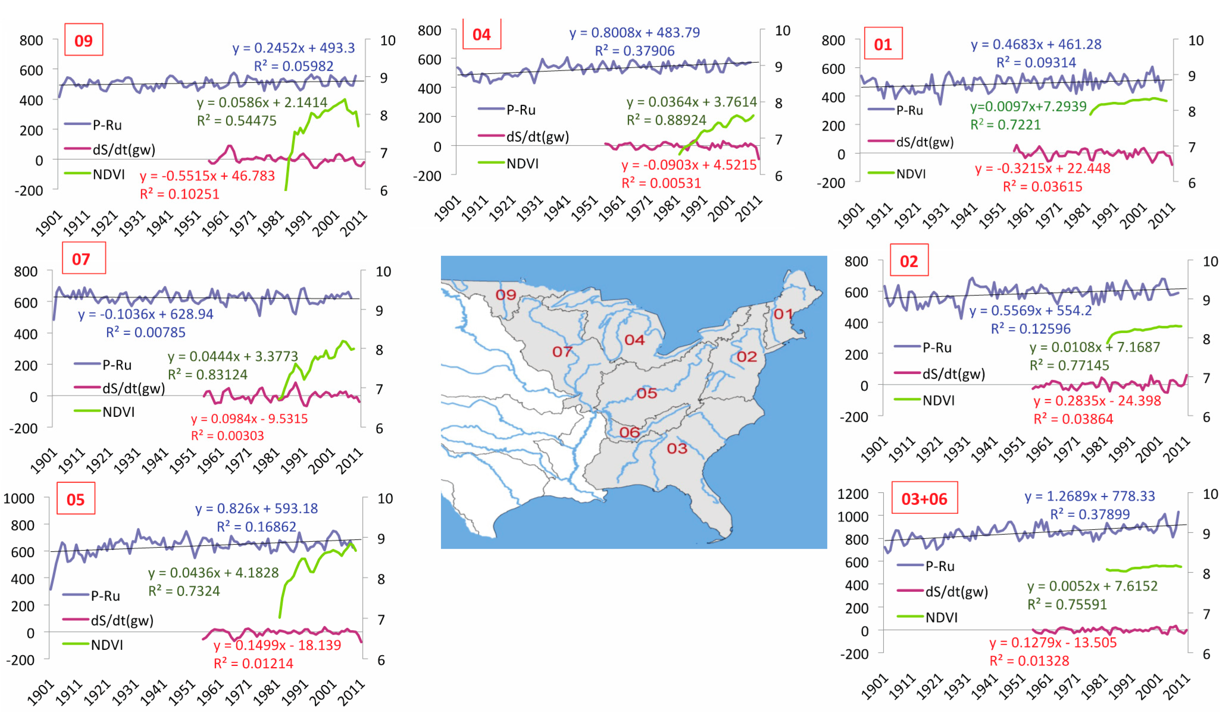
3.1. Inter-Hydrological Unit Analysis

We first conduct a trend analysis of changes to the water budget components and vegetation greening at the hydrological unit scale to assess variability within the study region. The trend magnitudes can be estimated using different approaches, including Sen’s slope estimator or the ordinary least squares regression [39,40]. A two-tailed hypothesis test is used to determine the significance of these trends at the 95% confidence level. Time series of (P-Ru) from 1901–2008, dS/dt(gw) from 1955–2011 and NDVI from 1982–2009 are displayed in Figure 2 for each hydrological unit, and quantitative results of the trend and significance tests are provided in Table 1. The longest possible time series for each variable is used, given the available data. Hydrological unit 6 is considerably smaller in spatial scale than the other hydrological units in our study region. Therefore, in order to compare hydrological units of similar size, hydrological unit 6 and the adjacent hydrological unit 3 have been combined and are considered as one hydrological unit for the purpose of this analysis.
We use the Kendall-Sen slope estimator and the linear regression methods to estimate the magnitude of the trends for each individual hydrological unit. Both methods produce similar estimates. In all but one of the hydrological units (HU7), (P-Ru) trends are positive and statistically significant at the 95% confidence interval, indicating that P is increasing, and more so than Ru (Table 1). The largest increases in (P-Ru) occur in the eastern-most hydrological units, while HU’s 7 and 9, in the northwestern-most region of the study domain exhibit the smallest trends. Generally, however, P-Ru trends are similar across the hydrological units. In all but one hydrological unit, dS/dt(gw) trends are insignificant in the statistical sense, while NDVI trends are positive and significant for all hydrological units (Table 1). While some variability exists between the different hydrological units, the water budget components and vegetation trends are consistent across the study region, and inter-hydrological unit variability is limited.
Figure 2. Time series of P-Ru (mm∙yr−1) from 1901–2008, dS/dt(gw) (mm∙yr−1) from 1955–2011 (primary axis) and annual total NDVI (yr−1) from 1982–2009 (secondary axis) for each hydrological unit (HU) considered in the study region. Linear regression trend lines and R2 coefficients are displayed. Red-boxed numbers identify which HU each subplot corresponds to. Note, HU3 and HU6 are considered together as one hydrological unit. See text for further details.
Hydrology 02 00093 g002
Table 1. The rate of change in the difference between precipitation and runoff (P-Ru) in mm∙yr−1, groundwater storage (dS/dt(gw)) in mm∙yr−1 and Normalized Difference Vegetation Index (NDVI) in yr−1, for each Hydrological Unit (HU) considered in our study region. Linear regression and Kendall-Sen methods are used to estimate slopes. Significance is considered at the 95% confidence level.
P-RudS/dt(gw)NDVI
Linear slopeKendall slopeLinear slopeKendall slopeLinear slopeKendall slope
[p-value][p-value][p-value][p-value][p-value][p-value]
HU010.470.43−0.31−0.220.010.01
[0.0013][0.0041][0.1935][0.3182][1.91(10)−9][7.77(10)−9]
HU020.560.520.250.30.010.01
[0.0002][0.0013][0.2140][0.1464][8.59(10)−13][2.05(10)−11]
HU03+061.271.230.150.160.010.01
[1.33(10)−12][1.96(10)−11][0.3474][0.4366][1.58(10)−9][1.40(10)−6]
HU040.800.81−0.06−0.030.040.04
[1.33(10)−12][6.90(10)−11][0.7129][0.8096][2.97(10)−13][4.87(10)−10]
HU050.830.560.070.040.040.04
[1.00(10)−5][1.40(10)−3][0.7223][0.7990][9.98(10)−10][3.02(10)−9]
HU07−0.10−0.100.100.180.040.04
[0.3618][0.3250][0.6892][0.4614][7.51(10)−11][7.93(10)−9]
HU090.250.22−0.61−0.370.060.05
[0.0107][0.0180][0.0094][0.0702][1.00(10)−5][7.81(10)−7]
The small inter-hydrological unit variability is indicative of the homogeneity of the study region in terms of changes in (P-Ru), dS/dt(gw) and NDVI. Therefore in the following sections, these quantities are averaged over the study region where the analysis of the trend in ET is carried out as a residual from the components of the water budget.

3.2. Study Region Analysis

In order to estimate ET trends over the study region, we aggregate the precipitation, runoff, groundwater storage and NDVI data over the entire study region represented in Figure 1. Similar to the analysis in Section 3.1, a three-year running average was applied to all time series.
Time series of P, Ru, dS/dt(gw) and NDVI, as well as their respective intra-regional variation, for the period of analysis are shown in Figure 3 and are used in the following analyses. We use the sample mean standard deviation across all hydrological units to represent the intra-regional variation (V), calculated as:
V = σ n
where σ is the standard deviation of all values in a given year and n is the number of hydrological units, since the annual mean calculations consist of one value per hydrological unit. This measure was added to, and subtracted from, the mean value for a given year to provide the spread displayed in Figure 3.

3.2.1. Precipitation and Runoff Trends

Using the linear regression approach, we find the trend in P and (P-Ru) to be positive and statistically significant at the 95% confidence level, but not the trend in Ru (p = 0.55). The use of the Kendall-Sen slope estimator leads to similar results. The regression analysis shows precipitation has increased annually by about 0.67 mm∙yr−1 while (P-Ru) has increased annually by 0.55 mm∙yr−1 (Table 2). This corresponds to a (P-Ru) increase from an average of 529 mm∙yr−1 in the first decade of the 20th century to 593 mm∙yr−1 in the first decade of the 21st century, an increase of about 11.4%. Combined, these results robustly indicate that the increase in (P-Ru) is mainly due to increase in P and that this increase has not been entirely directed to Ru, thus leaving some “excess water” unaccounted for.
Figure 3. Observed annual (a) precipitation (mm∙yr−1) and runoff (mm∙yr−1) for 1901 to 2008, (b) change in groundwater storage (mm∙yr−1) for 1955 to 2011 and (c) NDVI (dimensionless) for 1982 to 2009. The shaded area shows the mean ± sample mean standard deviation (Equation (2)). Observations are averaged for the eastern United States. See text for details.
Hydrology 02 00093 g003

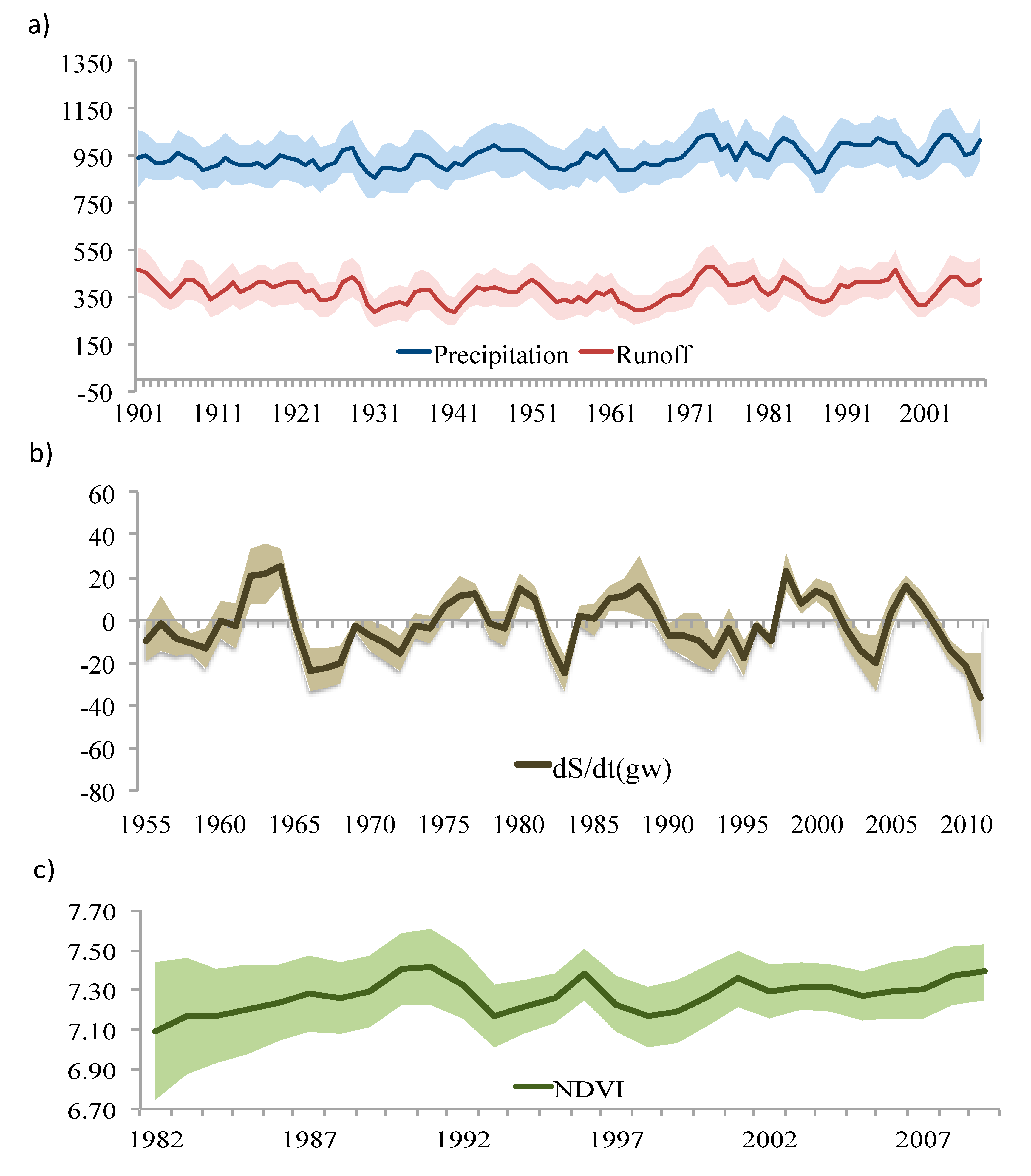
3.2.2. Groundwater Storage and NDVI Trends

Although groundwater is constantly replenished by precipitation that infiltrates into aquifers, change in groundwater storage, dS/dt(gw), has had a negligible response to the “excess water” associated with (P-Ru). Our analysis of groundwater averaged over the study region indicates a slightly decreasing trend. Similar to runoff, a trend detection analysis indicates that this trend in the annual dS/dt(gw) is not significant (p = 601) in the statistical sense (Figure 3 and Table 2). Other work [41] suggests that areas in the northern New England and the South Atlantic-Gulf regions experienced prolonged declines in groundwater levels, but also suggests increases in most other regions, resulting in an uncertain trend for the entire region over the period extending from 1940 to 2007.
Our analysis indicates a positive and statistically significant trend in vegetation greening (NDVI) over the study region.
Table 2. The rate of change calculated from linear regression and the Kendall Sen slope estimator, along with the respective p-values. The units for the slopes of precipitation, runoff and the difference (P-Ru) are given in mm∙yr−1. Annual changes in dS/dt(gw) (mm∙yr−1) and NDVI (dimensionless) are also listed.
Linear regression slopep-valueKendall-Sen slopeMann-Kendall p-value
Precipitation0.674.40(10)−80.671.27(10)−6
Runoff0.120.54950.110.4429
Difference (P-Ru)0.554.44(10)−90.542.22(10)−8
dS/dt(gw)−0.060.6009−0.010.9506
NDVI0.0040.03520.0060.0058

3.3. Excess Water Analysis

As indicated in Table 2 and Figure 3, (P-Ru) is generally increasing, and dS/dt(gw) changes do not fully compensate for these trends, since change in this quantity is shown to be negligible for most hydrological units in the study region, and over the total area. Quantifying the cumulative amount of the “excess water” from 1901 to 2008, which we can attribute to increases in P outpacing increases in Ru, further illustrates that water storage components have not fully accounted for rising (P-Ru) trends. We estimated the total amount of water produced by the observed difference between precipitation and runoff (P-Ru) over the study area and over time. To minimize the effects of interannual variations in (P-Ru), we used a linear fit from Table 2 to estimate the baseline (P-Ru) in 1901 as 506 mm∙yr−1. The total excess water accumulated above this baseline from 1901 to 2008 was then obtained by integrating (P-Ru) over the 108 years and was estimated to be 3.18 m.
We consider which components of the water budget could account for this excess water associated with (P-Ru).

3.3.1. Change in Surface Storage

If this excess water were entirely attributed to surface storage, the entire study area would be submerged under 3.18 m of water. As a comparison, we collected the surface storage specifications of all dams located in the 30 states encompassing our study area that are monitored by the National Inventory of Dams [42]. We estimated that even if each dam were filled to maximum capacity entirely by excess water from (P-Ru), this would still only account for 0.24 m, or 7.6%, of the total 3.18 m of the excess water. This is in agreement with the studies [19,20] that have shown that changes in surface water storage dS/dt(sw) and storage in unsaturated zone dS/dt(uz) are small and negligible over decadal to century time scales. Therefore we conclude changes in surface storage and unsaturated zone storage can only explain, a small fraction, if any, of the increasing (P-Ru) trends.

3.3.2. Change in Groundwater Storage

Using the same cumulative water amount and an average specific yield of 0.15 provided by [31], if the excess water was directed to dS/dt(gw) in its entirety, the water table would have been forced to rise 21.2 m. Considering our previous analysis, using wells data, showed that there has not been a significant increase in water levels over the domain during our period of analysis, we also conclude that groundwater storage must only account for a fraction of the excess water.
To further illustrate that change in groundwater storage alone cannot account for the total excess water generated by (P-Ru), we consider that the amount of water withdrawn in 1980, a record high single-year withdrawal amount [43], was withdrawn each individual year from 1901 to 2008. Using the value of total US groundwater withdrawal in 1980 and the percent of total withdrawal contribution from each hydrological unit [44], we estimated an amount for the study area of 46,543 million gallons per day. We applied this value to each year of our study period and divided by the study domain area of 3.57 × 10 12 m2 to estimate the depth of the water withdrawal. We determined this maximum, overestimated groundwater withdrawal to be about 1.93 m in depth. Even if this entire withdrawn amount were restored as water storage, it would only represent about 61% of the 3.18 m of the excess water.
This analysis leads to the reasonable conclusion that storage changes alone cannot account for of the totality of the observed (P-Ru) difference, even given vast overestimations of these storage changes. Therefore, other components of the water budget must have also responded to the observed (P-Ru) trends.

3.4. Trends in Human Water Use

For the study region, USGS statistics [38] indicate that the total water withdrawal for human use is about 140,471 million gallons per day in 2005 (Table 3). It also indicates that water withdrawal amounts vary by water use category, with thermoelectric power using the highest amount followed by public supply, industrial use, and irrigation. However, not all of these amounts are consumptive water. Consumptive water is defined as the water removed from available supplies without return to a water resource system. For example, the water used in manufacturing, or for food preparation that is not returned to a stream is considered consumptive. Human activities have different rates of consumptive water. For example, although a large amount of water is withdrawn for use in thermoelectric power generation, only 2.5% of it is consumptive [45]. Table 3 shows the different rates of consumptive water [46] for the different water use categories listed for our study area.
Using these rates and the water withdrawal amounts provided by the USGS, we estimate that from the total human water use, about 4.67 mm, or 10.4% was consumptive water in the study region in 2005 (Table 3). This value is in good agreement with the USGS study in [47], which shows a 10% consumptive water rate as an upper limit for the study area in 1983.
It is to be noted that in the study area, irrigated lands constitute only a small fraction of total land use [24], yet this land use type constitutes the second most amount of consumptive water use among the categories defined in Table 3.
Table 3. Water withdrawal by water-use category for the U.S. states east of the Mississippi river for 2005 from the USGS [38]. We use the total area of the study region ( 3.57 × 10 12 m2) to convert the unit from gallons/day to mm/year. Numbers in brackets are references to the percent consumptive water use categories listed for our regions.
CategoryWithdraw million gallons/dayPercent consumptive waterConsumptive water million gallons/dayConsumptive water mm∙yr−1
Thermo-electric Power94,7012.5% [46]23680.78
Public Supply + Domestic23,25823% [46]53491.76
Industrial907314% [46]12700.42
Irrigation787656% [46]44111.45
Aquaculture3787N/A [46]N/AN/A
Mining110621% [46]3430.11
Livestock67168% [46]4560.15
Total140,47114,1974.67
If we apply the 2005 consumptive water amount to the entire 108-year period of analysis, the total amount of consumptive water over the study area and over time would be 0.51 m in depth. Applying the 2005 consumptive water rate to all years is an overestimation since consumption rates were presumably smaller in the earlier years of the studied time period, when the population was smaller. Furthermore, following this logic, the underestimated period (2006–2008), with presumably higher population, is very short compared to the overestimated period (1901–2005). Finally, taking the overestimated storage amount into account, in addition to the overestimated consumptive water amount, there will still be 0.50 m of excess water unaccounted for (Table 4).
Table 4. Components of the hydrological cycle (m) over the period of analysis. Storage represents the total of the estimated maximum surface water (0.24 m) and groundwater (1.93 m) storage terms. The storage and consumptive water amounts are deliberate overestimates, contributing to an underestimate of the excess water that accumulated during the period of study. See text for details.
(P-Ru) AccumulationStorageConsumptive WaterResidual
3.182.170.510.50
In the eastern US, measured ET using lysimeters has been shown to reach roughly 0.83 m∙yr−1 [48]. Using this value as a baseline of annual ET rate over the study area, to remove 0.50 m of excess water over 108 years ( 4.63 × 10 3 m∙yr−1), we estimate ET must have increased with an annual average rate of 0.56%, obtained by dividing the 4.63 × 10 3 m∙yr−1 by the baseline, over the study period.
While we do not consider this an exact value of an ET rate of change, it is an estimated value that indicates ET has increased during our period of analysis, even given large overestimations of water storage and consumption changes.

3.5. Evapotranspiration

Given the spatial and temporal scale of our work and the analysis of uncertainties associated with the different components of the hydrological cycle, our analysis concludes that the trend in (P-Ru) is statistically significant at the 95% confidence level. Furthermore, even when extremely overestimated, changes in all three storage components (dS/dt(sw), dS/dt(uz) and dS/dt(gw)) do not account for the entirety of (P-Ru) changes, implying ET must have increased to maintain the region-scale water budget. Based on the more realistic trend analysis, storage changes are negligible, a conclusion in agreement with previous studies [49,50,51]. Despite uncertainties in estimates, both the overestimated storage analysis and the more rigorous trend analysis show ET has historically been increasing over the eastern United States.

3.6. Evapotranspiration and Vegetation Greening

We also examined to what extent vegetation greening, and consequently increases in ET, could be explained by increases in the “excess water” (P-Ru). Although coherent satellite observations of vegetation greening do not exist over the entire period of analysis, the longest available time series of AVHRR-observed NDVI [34] shows evidence of vegetation greening from 1982–2009 over all eight hydrological units considered in this study. A linear regression trend analysis showed that the average annual NDVI has a statistically significant positive trend of 0.004 per year over the 1982 to 2009 period (Table 2). These trends are in agreement with measurements made by the United States Forest Service, as documented in [52]. These observations indicated that vegetation density in timberland area, which makes up the majority of U.S. forests, has been increasing since 1953 in the Northeast and Southeast. The referenced findings incorporated measurements of growing stock, or the volume of living vegetation. Therefore, similar to our NDVI calculations, this positive trend only represents vegetation greening of previously existing plant life, and not an increase of vegetation areal extent.
The data show a statistically significant (p = 0.004) lag-correlation between changes in NDVI and excess water (P-Ru), where NDVI was lagged by one year to account for the natural response of NDVI to precipitation. A lag of weeks or months is a more accurate representation of the physical lag between available water and vegetation greening, and may have resulted in a higher correlation, but we are limited to annual runoff data given the time and space scale of our study. A lag of one year has been used in a similar fashion in previous work ([53,54]). The lag-correlation also shows that (P-Ru) explains only about 20% of the total variance in NDVI, reflecting the fact that other variables (e.g., temperature, nutrients, vegetation composition, growing season length and solar radiation) also control NDVI trends. Furthermore, NDVI is only indicative of an increase in transpiration and interception loss of water from the canopy, whereas the “excess water” contributes not just to evaporation from the canopy, but also to soil evaporation. Biophysical modeling of evapotranspiration shows that over the study area, the canopy-dependent components of evaporation represent approximately 65% of the total evapotranspiration rate [55], in agreement with a multi-model average of 64% [56], suggesting that over vegetated lands, an increase in ET is largely due to vegetation growth through transpiration and interception loss. On the other hand, the relationship between vegetation CO2 uptake and transpiration is controlled by stomatal conductance. Increased CO2 reduces stomatal conductance, yet this reduction is not associated with similar change in stomatal density. Under elevated CO2, vegetation exhibits down-regulation characterized by a reduction in the initial CO2-enhanced rates of photosynthesis that results from a decrease in the activity and the amount of Rubisco [16]. In model simulations [12], down-regulation reduced the canopy conductance beyond the reduction caused by the radiative and physiological effects of CO2 leading to increased water availability which could be diverted to increase leaf density beyond increases caused by climate changes and CO2-induced water use efficiency. However, the exact moisture stressing mechanisms in the soil, plant and atmosphere are difficult to assess due to the strong nonlinear correlations among environmental forcing variables on transpiration [57], which could explain why the “excess water” can only explain a fraction of the variance in NDVI, even though a strong correlation exists between the two variables (r = 0.45). Our results merely hint at the possibility of a physical relationship. Further analysis is necessary to draw more robust conclusions.
It is difficult to precisely separate the different components of the water budget on such large scales and this analysis is an attempt to highlight the dynamic interaction between vegetation and climate in the regulation of the water balance and the partitioning of precipitation into evapotranspiration and runoff. The statistical relationship establishes observational evidence supporting the hypothesis that vegetation greening is responding to the increased precipitation and suggests that part of the “excess water” is contributing to increases in evapotranspiration.

4. Conclusions

Based on a century-scale observational analysis over large hydrological units of the Eastern United States, we find that increase in precipitation led to an increase in evapotranspiration during the twentieth century, possibly, in part, through vegetation greening. We observed that precipitation increased during our study period (1901–2008), and more so than runoff across most hydrological units and averaged over the large study area. We determined that changes in water storage were negligible and, taking into account anthropogenic water use, estimated that ET had a positive trend during this time period. We also showed a statistically significant correlation between increasing NVDI and (P-Ru) trends, indicating that this vegetation greening as measured by NDVI may have been partially responsible for the positive ET trend.
Projected increases in global temperature, and accompanying regional increases in land precipitation, are supported by observations [1]. An increase in land precipitation will increase soil moisture; and where vegetation growth was previously water-limited, canopy greening will occur. Where this happens, evapotranspiration will also increase, leading to surface air temperature cooling and supporting the negative feedback in climate simulations with elevated CO2 as suggested in [5,6]. This claim is reinforced by results from the Intergovernmental Panel on Climate Change [1], which shows no significant trend to increases in surface temperature in the Mississippi River basin and areas east over the past 100 years. The same results show warming has occurred in the northeast US region roughly corresponding to hydrological units 1 and 2, however. In agreement with our observations, modeling studies [58] indicate that in central North America, vegetation greening is essentially due to increase in precipitation. Our analysis lends weight to the notion that, in tandem with external factors such as agriculture intensification [59], the additional water available from increasing precipitation associated with an increase in CO2 and climate change, stimulates vegetation growth ([6] and references therein). This effect introduces a negative feedback with important implications for the climate and the carbon cycle. The feedback increases carbon sequestration through vegetation growth and enhances evapotranspiration rates, thus cooling the air.
This process has been modeled under increased CO2 conditions through various studies [5,6,7]. The results showed that the magnitude of the projected cooling depended partly on the treatment of the vegetation physiological activity under increased CO2 concentration and the associated climate change, and partly on the nature of the locally dominant surface-atmosphere interaction, both of which are highly model dependent. This study establishes an observational basis for this hypothesis, which should be included in all climate models projecting the future state of climate under an increased CO2 concentration.
We consider this study to be a preliminary observational analysis and a more detailed analysis of the relationship between excess water and vegetation greening is warranted. Although further work is necessary to solidify conclusions, results presented in this study suggest that changes in the state of vegetation may already be playing a role in the continental water and energy budget as atmospheric CO2 increases, possibly slowing the course of climate trends.

Acknowledgments

The authors thank Forrest Hall of the University of Maryland Baltimore County as well as Randal Koster and Piers Sellers of Goddard Space Flight Center for their comments and feedback on the manuscript. Funding for Lahouari Bounoua was provided by the NASA Land Cover and Land Use Change program. Funding for this work was provided to Thomas G. Huntington by NASA (grants NNH12AT17I, NNH04AA66I and NNH08A157I). Additional support was provided by the U.S. Geological Survey’s funds for the study of Climate and Land Use Change and by the NASA Land Cover Land Use Change program.

Author Contributions

Ryan J. Kramer retrieved and processed the well data and conducted the corresponding groundwater analysis. He also contributed to the presentation of the results, researching background information for the introduction, developing the structure of both the study and the manuscript, and contributed to the writing of every section of the manuscript. Lahouari Bounoua developed the scientific idea of this research paper, supervised and guided this work. He also helped retrieve and process many of the datasets used in this study, contributed to the analysis of the data and took part in the writing of every section of the article. Ping Zhang conducted the trend analyses and statistical tests used in this study. She also conducted the consumptive water analysis, helped develop the methodology, and wrote the results sections corresponding to this analysis. Robert E. Wolfe developed the consumptive water analysis, providing guidance for determining which aspects of water use should be considered in the water budget analysis. He also helped write the results and methodology sections corresponding to the consumptive water analysis. Thomas G. Huntington offered guidance about the various components of the water budget to study and the proper types of analyses to conduct. He also helped develop the water storage analysis and contributed to the writing of the article’s introduction, results and concluding remarks. Marc L. Imhoff helped with data analysis. He also contributed to the interpretation and summarization of the results in the article. Kurtis Thome contributed to the analysis of the data, interpretation of the results and helped develop many of the scientific ideas supporting this study. Genevieve L. Noyce contributed to the groundwater analysis and drafting of the introduction and results section of the article. All authors helped edit multiple drafts, offering comments and corrections.

Conflicts of Interest

The authors declare no conflict of interest.

References

  1. Stocker, T.F.; Qin, D.; Plattner, G.-K.; Tignor, M.; Allen, S.K.; Bosching, J.; Nauels, A.; Xia, Y.; Bex, V.; Midgley, P.M. Climate Change 2013: The Physical Science basis. In Proceedings of the Contribution of Working Group I to the Fifth Assessment Report of the IPCC, Stockholm, Sweden, 23–26 September 2013; Cambridge University Press: Cambridge, United Kingdon/New York, NY, USA, 2013. [Google Scholar]
  2. Dirmeyer, P.A.; Brubaker, K.L. Evidence for trends in the northern hemisphere water cycle. Geophys. Res. Lett. 2006, 33, L14712. [Google Scholar] [CrossRef]
  3. Held, I.M.; Soden, B.J. Robust responses of the hydrological cycle to global warming. J. Clim. 2006, 19, 5686–5699. [Google Scholar] [CrossRef]
  4. Huntington, T.G. Evidence for intensification of the global water cycle: Review and synthesis. J. Hydrol. 2006, 319, 83–95. [Google Scholar] [CrossRef]
  5. Betts, R.A.; Cox, P.M.; Lee, S.E.; Woodward, F.I. Contrasting physiological and structural vegetation feedbacks in climate change simulations. Nature 1997, 387, 796–799. [Google Scholar] [CrossRef]
  6. Bounoua, L.; Hall, F.G.; Sellers, P.J.; Kumar, A.; Collatz, G.J.; Tucker, C.J.; Imhoff, M.L. Quantifying the negative feedback of vegetation to greenhouse warming: A modeling approach. Geophys. Res. Lett. 2010, 37, L23701. [Google Scholar]
  7. Levis, S.; Foley, J.A.; Pollard, D. Large-scale vegetation feedbacks on a doubled CO2 climate. J. Clim. 2000, 13, 1313–1325. [Google Scholar] [CrossRef]
  8. Bonan, G.B. Forests and climate change: Forcings, feedbacks, and the climate benefits of forests. Science 2008, 320, 1444–1449. [Google Scholar] [CrossRef] [PubMed]
  9. Bounoua, L.; Collatz, G.J.; Los, S.O.; Sellers, P.J. Sensitivity of climate to changes in NDVI. J. Clim. 2000, 13, 2277–2292. [Google Scholar] [CrossRef]
  10. Guillevic, P.; Koster, R.D.; Suarez, M.J.; Bounoua, L.; Collatz, G.J.; Los, S.O.; Mahanama, S.P.P. Influence of the interannual variability of vegetation on the surface energy balance—A global sensitivity study. J. Hydrometeorol. 2002, 3, 617–629. [Google Scholar] [CrossRef]
  11. Bounoua, L.; Collatz, G.J.; Sellers, P.J.; Randall, D.A. Interactions between vegetation and climate: Radiative and physiological effects of doubled atmospheric CO2. J. Clim. 1999, 12, 309–324. [Google Scholar] [CrossRef]
  12. Sellers, P.J.; Field, C.B.; Jensen, T.G.; Bounoua, L.; Collatz, G.J.; Randall, D.A.; Dazlich, D.A.; Los, S.O.; Berry, J.A.; Fung, I.; et al. Comparison of radiative and physiological effects of doubled atmospheric CO2 on climate. Science 1996, 271, 1402–1406. [Google Scholar] [CrossRef]
  13. Granier, A.; Bernhofer, C.; Buchmann, N.; Facini, O.; Grassi, G.; Heinesch, B.; Ilvesniemi, H.; Keronen, P.; Knohl, A.; Köstner, B.; et al. Evidence for soil water control on carbon and water dynamics in european forests during the extremely dry year: 2003. Agric. Forest Meteorol. 2007, 143, 123–145. [Google Scholar] [CrossRef]
  14. Hobbins, M.T.; Ramírez, J.A.; Brown, T.C. Trends in pan evaporation and actual evapotranspiration across the conterminous U.S.: Paradoxical or complementary? Geophys. Res. Lett. 2004, 31, L13503. [Google Scholar] [CrossRef]
  15. Nohara, D.; Kitoh, A.; Hosaka, M.; Oki, T. Impact of climate change on river discharge projected by multimodel ensemble. J. Hydrometeorol. 2006, 7, 1076–1089. [Google Scholar] [CrossRef]
  16. Leakey, A.D.; Ainsworth, E.A.; Bernacchi, C.J.; Rogers, A.; Long, S.P.; Ort, D.R. Elevated CO2 effects on plant carbon, nitrogen, and water relations: Six important lessons from FACE. J. Exp. Bot. 2009, 60, 2859–2876. [Google Scholar] [CrossRef] [PubMed]
  17. Healy, R.W.; Winter, T.C.; LaBaugh, J.W.; Franke, O.L. Water Budgets: Foundations for Effective Water-resources and Environmental Management; U.S. Geological Survey Circular 1308; U.S. Geological Survey: Reston, VA, USA, 2007; p. 90.
  18. Scanlon, B.R.; Healy, R.W.; Cook, P.G. Choosing appropriate techniques for quantifying groundwater recharge. Hydrogeol. J. 2002, 10, 18–39. [Google Scholar] [CrossRef]
  19. Domokos, M.; Sass, J. Long-term water balances for subcatchments and partial national areas in the Danube Basin. J. Hydrol. 1990, 112, 267–292. [Google Scholar] [CrossRef]
  20. Gao, H.; Tang, Q.; Ferguson, C.; Wood, E.; Lettenmaier, D. Estimating the water budget of major US river basins via remote sensing. Int. J. Remote Sens. 2010, 31, 3955–3978. [Google Scholar] [CrossRef]
  21. Postel, S.L.; Daily, G.C.; Ehrlich, P.R. Human appropriation of renewable fresh water. Science 1996, 271, 785–788. [Google Scholar] [CrossRef]
  22. Milly, P.C.D.; Dunne, K.A. Trends in evaporation and surface cooling in the mississippi river basin. Geophys. Res. Lett. 2001, 28, 1219–1222. [Google Scholar] [CrossRef]
  23. Monfreda, C.; Ramankutty, N.; Foley, J.A. Farming the planet: 2. Geographic distribution of crop areas, yields, physiological types, and net primary production in the year 2000. Glob. Biogeochem. Cycles 2008, 22, GB1022. [Google Scholar] [CrossRef]
  24. Hutson, S.S.; Barber, N.L.; Kenny, J.F.; Linsey, K.S.; Lumia, D.S.; Maupin, M.A. Estimated Use of Water in the United States in 2000; U.S. Geological Survey Circular 1268; U.S. Geological Survey: Reston, VA, USA, 2004; p. 46.
  25. Teuling, A.J.; Hirschi, M.; Ohmura, A.; Wild, M.; Reichstein, M.; Ciais, P.; Buchmann, N.; Ammann, C.; Montagnani, L.; Richardson, A.D.; et al. A regional perspective on trends in continental evaporation. Geophys. Res. Lett. 2009. [Google Scholar] [CrossRef]
  26. USGS. USGS Waterwatch; U.S. Geological Survey: Reston, VA, USA, 2011.
  27. Schneider, U.; Becker, A.; Finger, P.; Meyer-Christoffer, A.; Ziese, M.; Rudolf, B. Gpcc’s new land surface precipitation climatology based on quality-controlled in situ data and its role in quantifying the global water cycle. Theor. Appl. Climatol. 2013, 115, 15–40. [Google Scholar] [CrossRef]
  28. Rodell, M.; Chen, J.; Kato, H.; Famiglietti, J.S.; Nigro, J.; Wilson, C.R. Estimating groundwater storage changes in the Mississippi River basin (USA) using GRACE. Hydrogeol. J. 2007, 15, 159–166. [Google Scholar] [CrossRef]
  29. Weider, K.; Boutt, D.F. Heterogeneous water table response to climate revealed by 60 years of ground water data. Geophys. Res. Lett. 2010. [Google Scholar] [CrossRef]
  30. USGS. USGS Climate Response Network; U.S. Geological Survey: Reston, VA, USA, 2011.
  31. Healy, R.W.; Cook, P.G. Using groundwater levels to estimate recharge. Hydrogeol. J. 2002, 10, 91–109. [Google Scholar] [CrossRef]
  32. Johnson, A.I. Specific Yield—Compilation of Specific Yields for Various Materials; U.S. Geological Survey Water Supply Paper; U.S. Geological Survey: Reston, VA, USA, 1967; Volume 1662-D.
  33. Morris, D.A.; Johnson, A.I. Summary of Hydrologic and Physical Properties of Rock and Soil Materials as Analyzed by the Hydrologic Laboratory of the U.S. Geological Survey 1948–1960; U.S. Geological Survey Water Supply Paper: Reston, VA, USA, 1967; Volume 1839-D.
  34. Tucker, C.; Pinzon, J.; Brown, M.; Slayback, D.; Pak, E.; Mahoney, R.; Vermote, E.; El Saleous, N. An extended AVHRR 8-km NDVI dataset compatible with MODIS and SPOT vegetation NDVI data. Int. J. Remote Sens. 2005, 26, 4485–4498. [Google Scholar] [CrossRef]
  35. Gitelson, A.A.; Kogan, F.; Zakarin, E.; Spivak, L.; Lebed, L. Using AVHRR data for quantitive estimation of vegetation conditions: Calibration and validation. Adv. Space Res. 1998, 22, 673–676. [Google Scholar] [CrossRef]
  36. Hansen, M.C.; Defries, R.S.; Townshend, J.R.G.; Sohlberg, R. Global land cover classification at 1 km spatial resolution using a classification tree approach. Int. J. Remote Sens. 2000, 21, 1331–1364. [Google Scholar] [CrossRef]
  37. Keenan, T.F.; Gray, J.; Friedl, M.A.; Toomey, M.; Bohrer, G.; Hollinger, D.Y.; Munger, J.W.; O’Keefe, J.; Schmid, H.P.; Wing, I.S.; et al. Net carbon uptake has increased through warming-induced changes in temperate forest phenology. Nat. Clim. Chang. 2014, 4, 598–604. [Google Scholar] [CrossRef]
  38. Kenny, J.F.; Barber, N.L.; Hutson, S.S.; Linsey, K.S.; Lovelace, J.K.; Maupin, M.A. Estimated Water Use in the United States in 2005; U.S. Geological Survey Circular 1344: Reston, VA, USA, 2009; p. 52.
  39. Daughney, C.; Reeves, R. Analysis of temporal trends in new zealand’s groundwater quality based on data from the National Groundwater Monitoring Programme. J. Hydrol. (New Zealand) 2006, 45, 41–62. [Google Scholar]
  40. Hess, A.; Iyer, H.; Malm, W. Linear trend analysis: A comparison of methods. Atmos. Environ. 2001, 35, 5211–5222. [Google Scholar] [CrossRef]
  41. Brutsaert, W. Annual drought flow and groundwater storage trends in the eastern half of the United States during the past two-third century. Theor. Appl. Climatol. 2010, 100, 93–103. [Google Scholar] [CrossRef]
  42. US Army Corps of Engineers (Ed.) National Inventory of Dams. 2009. Available online: http://nid.usace.army.mil/cm_apex/f?p=838:12 (accessed on 12 May 2015).
  43. Gleick, P.; Haasz, D.; Cain, N. The World’s Water 2004–2005: The Biennial Report on Freshwater Resources; Island Press: Washington, DC, USA, 2004; Volume 200405. [Google Scholar]
  44. Solley, W.B.; Pierce, R.R.; Perlman, H.A. Estimated Use of Water in the United States in 1995; U.S. Geological Survey Circular 1200: Reston, VA, USA, 1998; p. 52.
  45. Torcellini, P.A.; Long, N.; Judkoff, R. Consumptive Water Use for US Power Production; National Renewable Energy Laboratory: Golden, CO, USA, 2003; p. 14. [Google Scholar]
  46. Solley, W.B.; Pierce, R.R.; Perlman, H.A. Estimated Use of Water in the United States in 1990; U.S. Geological Survey Circular 1081: Reston, VA, USA, 1993; p. 56.
  47. National Water Summary—1983 Hydrologic Events and Issues; USGS (Ed.) U.S. Government Printing Office: Reston, VA, USA, 1984; p. 26.
  48. Van Bavel, C.H.M. Lysimetric measurements of evapotranspiration rates in the eastern United States. Soil Sci. Soc. Am. Proc. 1961, 25, 138–141. [Google Scholar] [CrossRef]
  49. Church, M.R.; Bishop, G.D.; Cassell, D.L. Maps of regional evapotranspiration and runoff/precipitation ratios in the northeast United States. J. Hydrol. 1995, 168, 283–298. [Google Scholar] [CrossRef]
  50. Lee, C.-H.; Chen, W.-P.; Lee, R.-H. Estimation of groundwater recharge using water balance coupled with base-flow-record estimation and stable-base-flow analysis. Environ. Geol. 2006, 51, 73–82. [Google Scholar] [CrossRef]
  51. Walter, M.T.; Wilks, D.S.; Parlange, J.-Y.; Schneider, R.L. Increasing evapotranspiration from the conterminous united states. J. Hydrometeorol. 2004, 5, 405–408. [Google Scholar] [CrossRef]
  52. Rautiainen, A.; Wernick, I.; Waggoner, P.E.; Ausubel, J.H.; Kauppi, P.E. A national and international analysis of changing forest density. PLoS ONE 2011, 6, e19577. [Google Scholar] [CrossRef] [PubMed]
  53. Martiny, N.; Richard, Y.; Camberlin, P. Inter-annual persistence effects in vegetation dynamics of semi-arid Africa. Geophys. Res. Lett. 2005, 32, L24403. [Google Scholar] [CrossRef]
  54. Camberlin, P.; Martiny, N.; Philippon, N.; Richard, Y. Determinants of the inter-annual relationships between remote sensed photosynthetic activity and rainfall in tropical africa. Remote Sens. Environ. 2007, 106, 199–216. [Google Scholar] [CrossRef]
  55. Bounoua, L.; Imhoff, M.L.; Franks, S. Irrigation Requirement Estimation Using MODIS Vegetation Indices and Inverse Biophysical Modeling. In Proceedings of IEEE International Geoscience & Remote Sensing Symposium, Barcelona, Spain, 24–29 July 2011.
  56. Dirmeyer, P.A.; Gao, X.; Zhao, M.; Guo, Z.; Oki, T.; Hanasaki, N. Gswp-2: Multimodel analysis and implications for our perception of the land surface. Bull. Am. Meteorol. Soc. 2006, 87, 1381–1397. [Google Scholar] [CrossRef]
  57. Pettijohn, J.C.; Salvucci, G.D.; Phillips, N.G.; Daley, M.J. Mechanisms of moisture stress in a mid-latitude temperate forest: Implications for feedforward and feedback controls from an irrigation experiment. Ecol. Model. 2009, 220, 968–978. [Google Scholar] [CrossRef]
  58. Piao, S.; Friedlingstein, P.; Ciais, P.; Zhou, L.; Chen, A. Effect of climate and CO2 changes on the greening of the Northern Hemisphere over the past two decades. Geophys. Res. Lett. 2006, 33, L23402. [Google Scholar] [CrossRef]
  59. Zeng, N.; Zhao, F.; Collatz, G.J.; Kalnay, E.; Salawitch, R.J.; West, T.O.; Guanter, L. Agricultural green revolution as a driver of increasing atmospheric CO2 seasonal amplitude. Nature 2014, 515, 394–397. [Google Scholar] [CrossRef] [PubMed]

