Development and Analyses of Artificial Intelligence (AI)-Based Models for the Flow Boiling Heat Transfer Coefficient of R600a in a Mini-Channel

Abstract

Environmental friendly refrigerants with zero ozone depletion potential (ODP) and zero global warming potential (GWP) are in great demand across the globe. One such popular refrigerant is isobutane (R600a) which, having zero ODP and negligible GWP, is considered in this study. This paper presents the two most popular artificial intelligence (AI) techniques, namely support vector regression (SVR) and artificial neural networks (ANN), to predict the heat transfer coefficient of refrigerant R600a. The independent input parameters of the models include mass flux, saturation temperature, heat flux, and vapor fraction. The heat transfer coefficient of R600a is the dependent output parameter. The prediction performance of these AI-based models is compared and validated against the experimental results, as well as with the existing correlations based on the statistical parameters. The SVR model based on the structural risk minimization (SRM) principle is observed to be superior compared with the other models and is more accurate, precise, and highly generalized; it has the lowest average absolute relative error (AARE) at 1.15% and the highest coefficient of determination (R²) at 0.9981. ANN gives an AARE of 5.14% and a R² value of 0.9685. Furthermore, the simulated results accurately predict the effect of input parameters on the heat transfer coefficient.

1. Introduction

The increasing demand for microelectronic devices in industrial and household applications, such as air-conditioning, refrigeration, and heat pumps, requires efficient heat removal techniques through micro- and mini-channels to resist high heat fluxes. Based on the hydraulic diameter, researchers have classified the flow channels as conventional channels (Dh ≥ 3 mm), mini-channels (3 mm ≥ Dh ≥ 200 μm), and micro-channels (200 μm ≥ Dh ≥ 10 μm) [1,2]. To better understand the boiling phenomenon in micro- and mini-channels, several studies have been done [3,4,5]. However, accurately modelling the boiling heat transfer coefficient in micro- and mini-channels is still a difficult task.

In the recent past, support vector machines (SVMs) have emerged as an artificial intelligence (AI) technique developed for classification purposes. However, its application has now been extended to regression [6,7,8]. Moreover, support vector regression (SVR) enjoys a lot of benefits over the traditional neural networks, such as the need to choose only a few parameters for modeling; avoiding over-fit to the data; and being a unique, global, and optimal solution.

In open literature, SVR has many applications for the prediction of many real-world problems, such as permeability predictions for hydrocarbon reservoirs [9], wind speed forecasting for wind farms [10], predicting for carbon monoxide in the atmosphere [11], predicting the heat transfer coefficient in a thermosiphon reboiler [12], and predicting heavy metal removal efficiency [13,14]. In the current study, the prediction of the heat transfer coefficient of the refrigerant R600a is made by using two artificial intelligence techniques (AI) namely, SVR and artificial neural networks (ANN). R600a is an environment-friendly natural refrigerant having 0 ODP and a low GWP of 3 [15,16].

2. Basic Idea of Support Vector Machines (SVMs)

A detailed description of an SVM can be found out in several works of literature [17,18,19]. The basic goal in a distinctive $\epsilon$-regression with the training samples P = {(m₁, n₁), (m₂, n₂), …, (m_N, n_N)} is to fit a function n = f(m) for a set of independent input variables m_i ϵ R^N and the corresponding dependent output variable n_i ϵ R^N.

The regression equation in the feature space can be given as

f (m,w) = (w●ϕ(m) + z)

(1)

where w is the weight vector, z is a constant, ϕ(m) is the feature function, and (w●ϕ(m)) is the dot product.

The regression is equivalent to minimizing the following equation

$$\mathrm{Minimize}:\mathrm{R}(f)=\mathrm{C}\frac{1}{N}{L}_{ϵ}\left(n,f\left(m,w\right)\right)+\frac{1}{2}||w^2||$$

(2)

$$L_{ϵ}\left(n,f\left(m,w\right)\right)=\{\begin{array}{cc}0& if \left|n-f\left(m,w\right)\right|\le \epsilon \\ \left|n-f\left(m,w\right)\right|-\epsilon & otherwise\end{array}$$

(3)

The first term in Equation (2) represents the empirical error, and the second term is the capacity or the complexity of the model. Term C in Equation (2) gives a measure of the optimization between the empirical error and the model complexity. Equation (3) defines a loss function called the $\epsilon$-insensitive loss function [20]. Furthermore, using Lagrangian multiplier α and α*, the optimization problem is converted into the dual problem. Only the non-zero coefficients, along with their corresponding input vectors, m_i, are called the support vectors. The final form is as follows

$$f(m,{\alpha }_i,{\alpha }_i^{\ast })={\sum }_{i=1}^{N_{sv}}\left({\alpha }_i-{\alpha }_i^{\ast }\right)\left(\varnothing \left(m_i\right)●\varnothing \left(m_j\right)\right)+z$$

(4)

With the help of kernel function K(m_i m_j), the SVR function can be obtained as shown below

$$f(m,{\alpha }_i,{\alpha }_i^{\ast })={\sum }_{i=1}^{N_{sv}}\left({\alpha }_i-{\alpha }_i^{\ast }\right)\mathrm{K}\left(m,m_i\right)+z$$

(5)

The term z or bias is obtained by using the Karush–Kuhn–Tucker conditions.

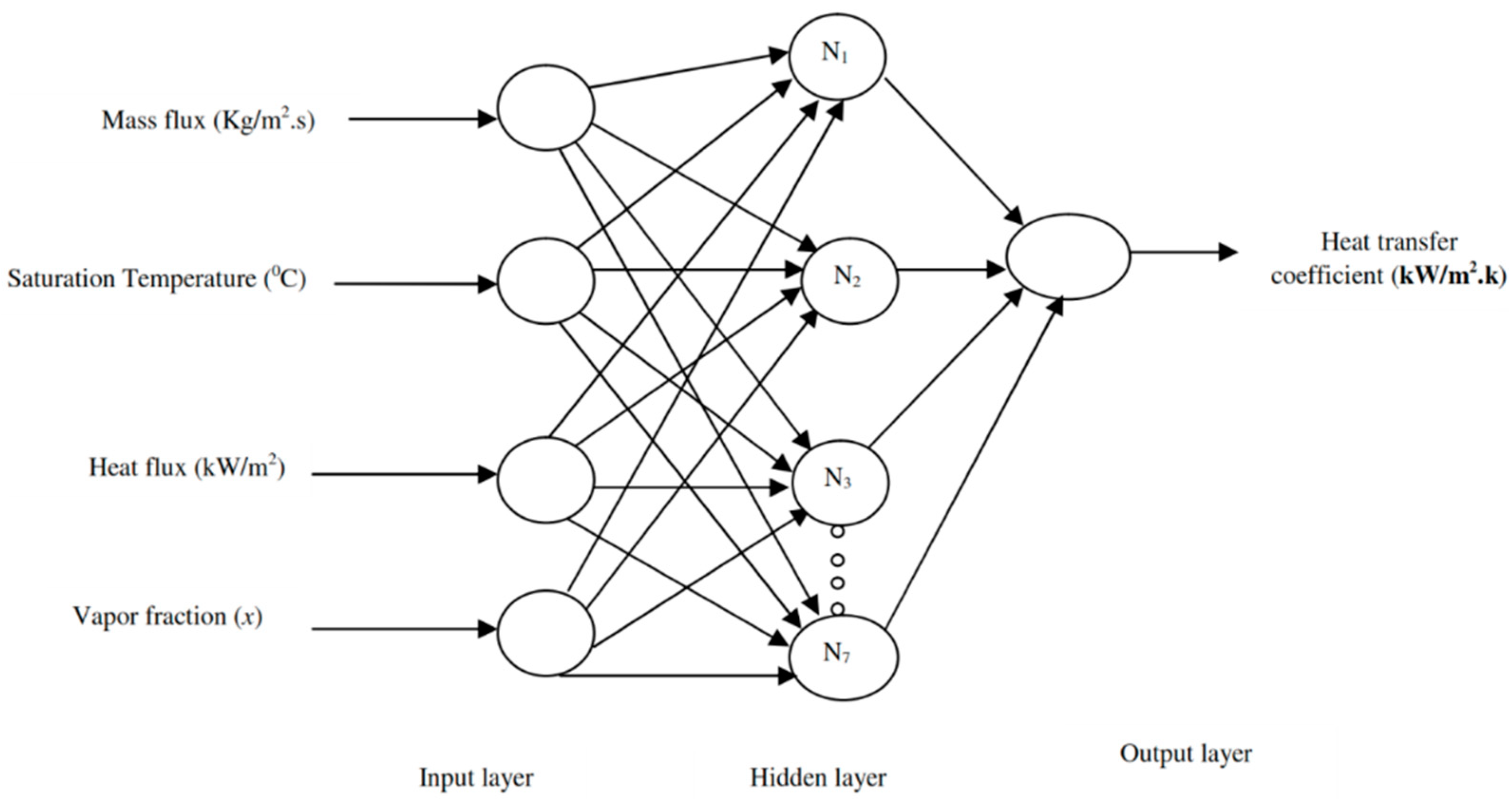
3. An Overview of ANNs

ANNs are parallel information processing systems which, to a large extent, emulate the human brain. It is composed of artificial neurons, nodes, or units. Furthermore, it has three layers: the input layer, the hidden layer, and the output layer. The input layer receives inputs from the outside environment and passes it to the hidden layer. The hidden layer transforms these inputs into a useable form via some non-linear activation function, and the signal goes to the output layer. The most commonly used activation functions are logistic (sigmoid), polynomial, linear, hyperbolic tangent, Gaussian function, and etc. [21]. The output layer thus presents the final model output. Generally, one hidden layer is sufficient to achieve the desired accuracy. Increasing the number of hidden layers increases the chances of over-fitting or under-fitting. Moreover, the number of neurons in the input and output layers are specified with respect to the input and output variable of a particular problem. However, the number of neurons in the hidden layer is unknown and needs to be specified. The optimal number of neurons at the hidden layers is found using a trial and error procedure. This optimal number produces the lowest value of mean square error (MSE) or the minimum value of residual variance, as an inappropriate number of neurons might lead to over-fitting/under-fitting of the model [22]. Based on the organization of neurons, ANNs are broadly classified into the feed-forward neural network and the feed-back neural network [23]. Employed in this study is a feed-forward neural network with a logistic activation function at the hidden layer and a linear activation function at the output layer.

4. An Overview of the Existing Correlations

A large number of correlations are available in the literature for predicting the heat transfer coefficient of various refrigerants. Some of them are listed below.

4.1. Magdalena Piasecka Correlation

Magdalena Piasecka [24] proposed the following correlation for FC-72, and this is given below

$$h=22.5•\Gamma •{\left(Pe•Bo\right)}^{0.64}•W{e}^{0.46}•\frac{K}{d_h},$$

(6)

where $\Gamma =0.028$.

Dimensionless numbers

$$Bo=q_w/G•h_{lv}, Pe=Re•Pr, Re=\left(G•d_h\right)/\mu , \mathrm{Pr}=\mu •Cp/K, We=G^2•d_h/\sigma$$

4.2. Dutkowski Correlation

The Dutkowski correlation [24,25] was developed for R134a and R-404a circular mini-channels, d_h = 0.45–2.30 mm, and has the following form

$$h=0.41R{e}_l^{0.848}•B{o}^{0.66}•C{o}^{-0.62}•{\left({\rho }_l/{\rho }_v\right)}^{1.28}$$

(7)

where $Co=\frac{1}{d_h}•\sqrt{\frac{\sigma }{g•\left({\rho }_l-{\rho }_v\right)}}.$

4.3. Li and Wu Correlation

The Li and Wu correlation [26] was developed for water, refrigerants, ethanol, propane, and CO₂. It is given below (d_h = 0.16–3.1 mm).

$$h=334B{o}^{0.3}•{\left(Bd•R{e}_l{}^{0.36}\right)}^{0.4}•\left(K_l/d_h\right)$$

(8)

where $Bd=\left[\left({\rho }_l-{\rho }_v\right)•d_h^2\right]/\sigma .$

5. Results and Discussion

In this study, SVR and ANN models have been developed using the experimental dataset comprising 319 data points taken from published literature [27]. DTREG software [28] was used to develop both the SVR and ANN models. These models have been developed for refrigerant R600a in a circular channel with an internal diameter of 1.1 mm covering a wide range of mass flux (G) from 200 to 800 Kg/m²·s, heat fluxes (q) ranging from 15 to 145 kW/m², saturation temperatures (T_sat) of 31 and 41 °C, and vapor qualities (x) from 0.05 to 0.95. The whole dataset of 319 samples was divided into 80% (255 data points) and 20% (64 data points), as the training dataset and the test dataset, respectively. Furthermore, a comparative study between ANN-based and SVR-based models is also presented in this research. The developed models were evaluated and validated against the experimental data based on statistical measures, such as R, AARE, RMSE, standard deviation (SD), mean absolute error (MAE), etc.

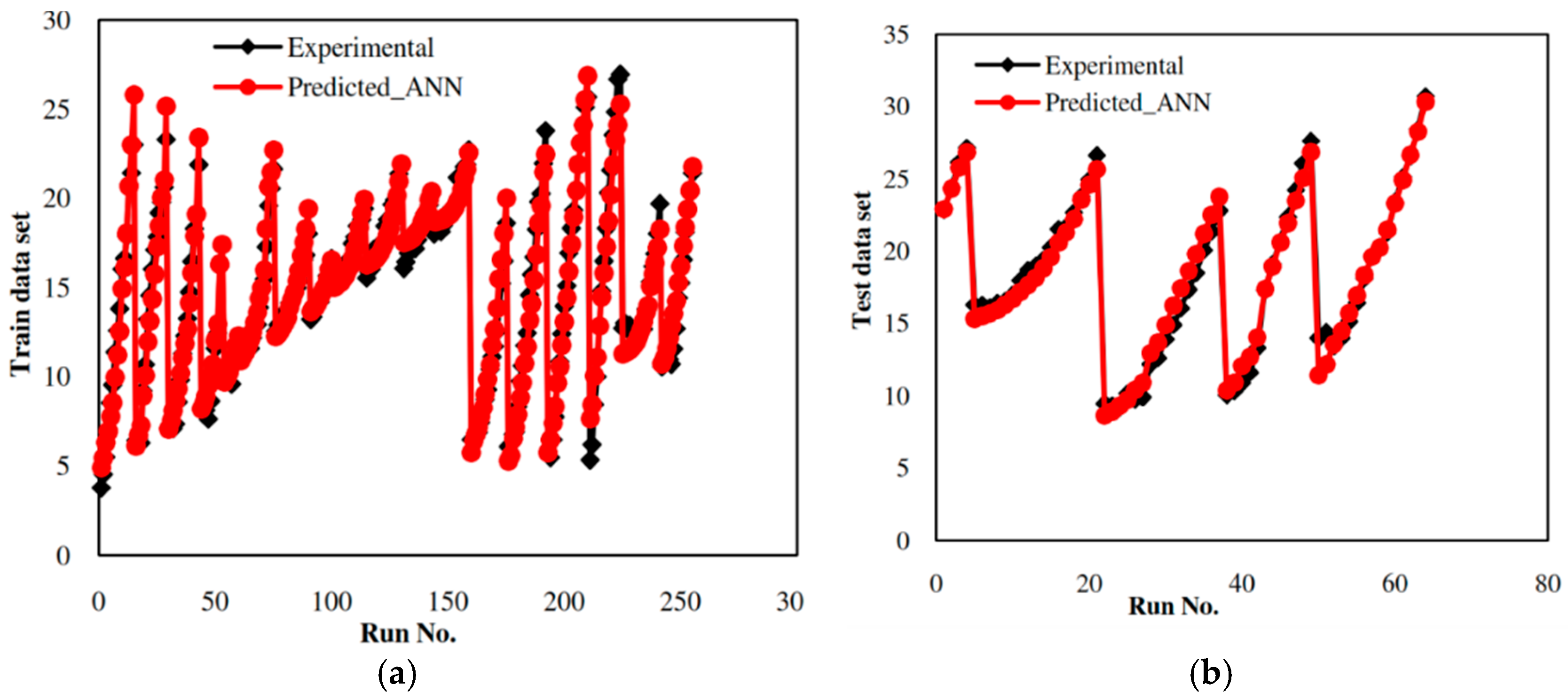
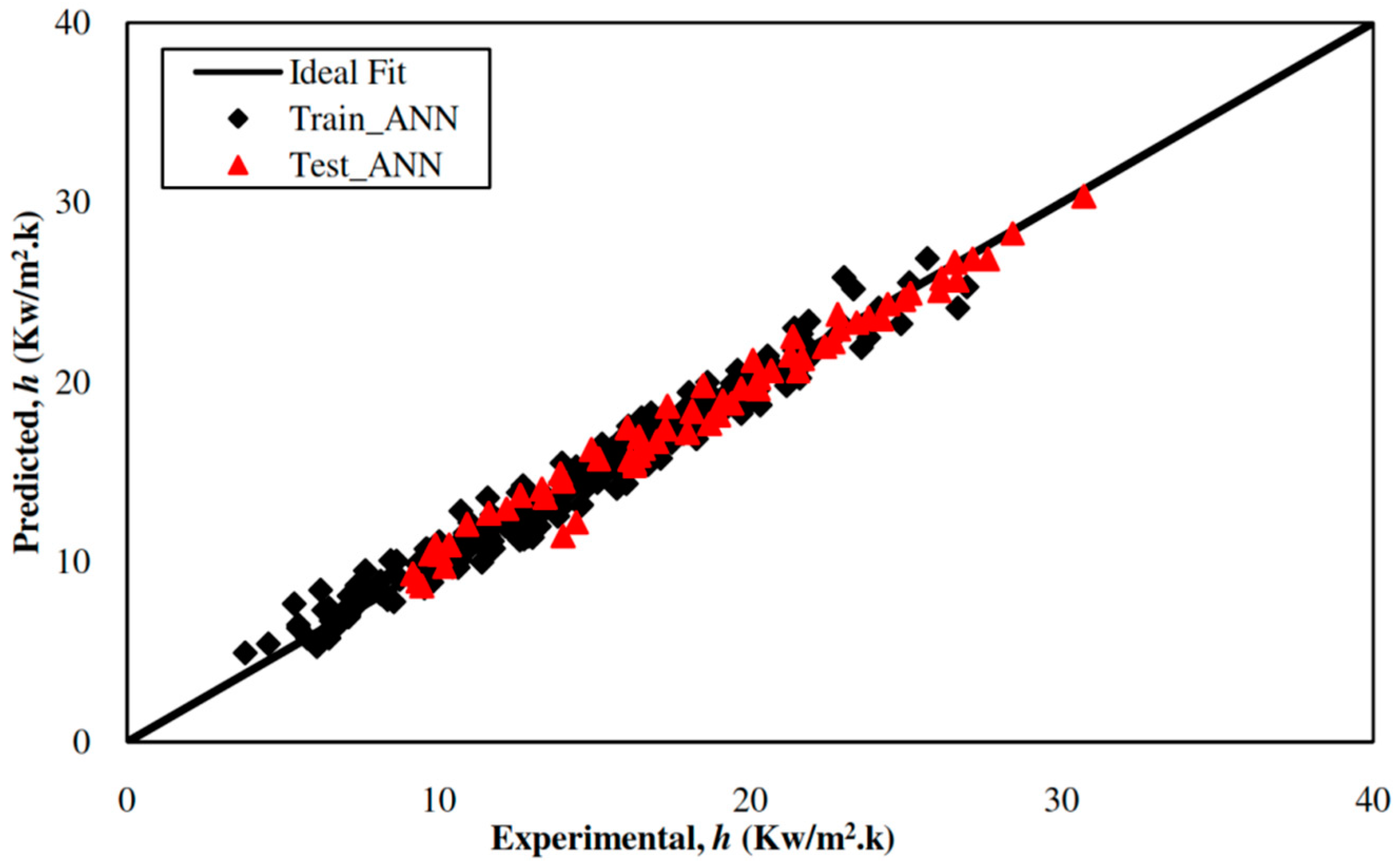
5.1. Development of the ANN-Based Model

The schematic representation of the multilayer perceptron neural network shown in Figure 1 is comprised of the input layer (independent variables), hidden layers, and the output layer (dependent/target variables). The optimum neural network structure of 4:7:1 has been found using the DTREG software. A three layered (4:7:1) feed-forward neural network has been used for modeling the heat transfer coefficient (h), with four neurons in the input layer for mass flux (G, kg/m²·s), saturation temperature (T_sat, °C), heat flux (q, kW/m²), and vapor fraction (x), seven neurons in one hidden layer, and one neuron for the heat transfer coefficient, h (kW/m²·k) in the output layer. The number of neurons at the input and output layers are set according to the particular type of problem, whereas the optimal number of hidden layer neurons is seven, and these give a minimum value of residual variance as shown in

Table 1. Optimum neurons at the hidden layer.

Hidden Layer 1 Neurons	% Residual Variance
2	8.27490
3	10.72571
4	4.03148
5	4.51386
6	8.74758
7	3.22918 (Optimal value)
8	3.99854
9	4.41057
10	6.25276
11	5.57635
12	4.74811
13	6.90271
14	4.34555
15	4.46499

. A logistic activation function at the hidden layer and linear activation function at the output layer has been used to develop the ANN model.

A training and test course curve has been constructed using the ANN model output as shown in Figure 2a,b, respectively. A comparison among the experimental and predicted values of the heat transfer coefficient of R600a via the ANN model using the training and test dataset is demonstrated in Figure 3.

Table 2. Evaluation of the ANN-based model based on statistical parameters.

Statistical Indices	Train Data	Test Data
AARE (%)	4.12	5.14
R	0.9884	0.9842
RMSE	0.8142	0.8608
SD	4.7469	5.2438
MRE	0.0412	0.0514
MAE (%)	1.02	1.05
Q2LOO (Train data), Q2ext (Test data)	0.9832	0.9685

exhibits the statistical evaluation parameters of the ANN model for both the training dataset and the test dataset. It is determined from this table that the ANN model has poor performance, especially because the test (unseen) dataset have high values of AARE (5.14%), RMSE (0.8608), MRE (0.0514), etc. ANN employs the empirical risk minimization principle (ERM) which minimizes only empirical error and does not consider the complexity of the model. As a result, it has a high accuracy for the training dataset and a low accuracy for the test (unseen) dataset.

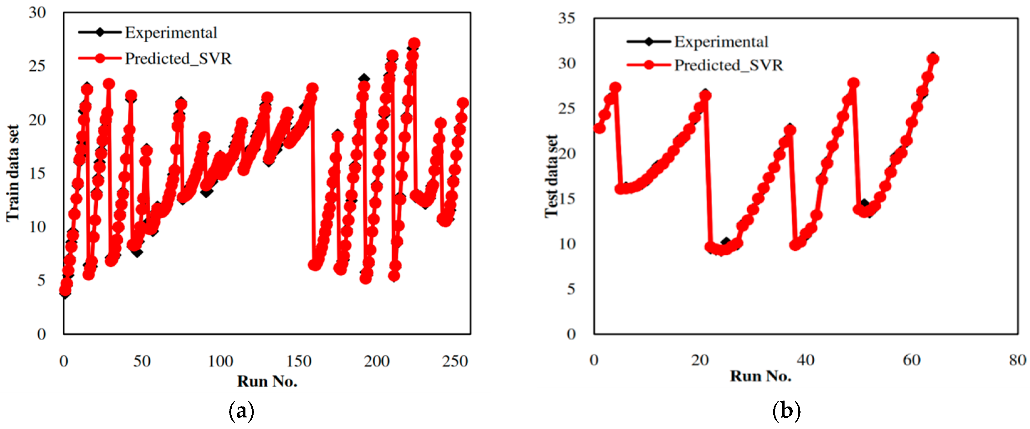
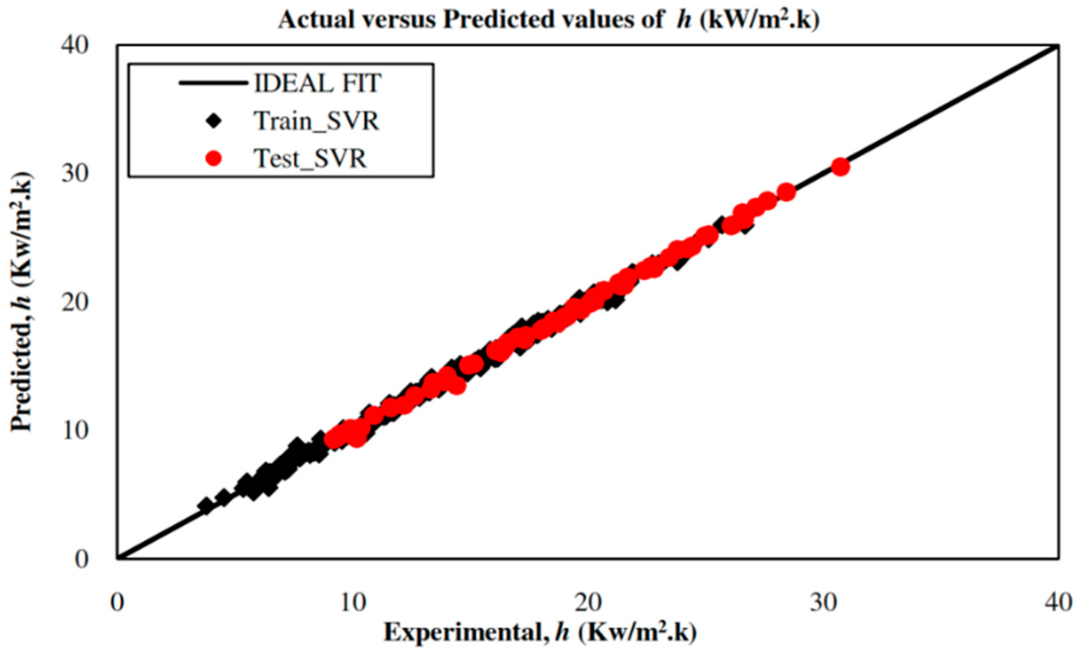
5.2. Development of an SVR-Based Model

The whole dataset is grouped into a dependent parameter (output/target) and independent input parameters for SVR modeling and then divided into two groups of 80% the total data (255 data points) and 20% the total data (64 data points) to create the training dataset and the test dataset, respectively. Among the various kernel functions—such as linear kernel, polynomial kernel, radial basis function (RBF) kernel, and sigmoid—the RBF kernel is chosen for its good general performance and only needing one parameter to be set [12,29].

Table 3. Optimal parameters of the SVR model for the prediction of heat transfer coefficient of R600a.

Model	C	γ = 1/2σ2	ε	Kernel Type	Loss Function	Number of Support Vectors	Number of Training Points
Heat transfer coefficient, h	4907.6	1.3486	0.001	RBF	ε-insensitive	175	255

gives the optimal measures of the SVR hyper-parameters C, ε, and the RBF kernel (γ) using the exhaustive grid search technique, which has 10-fold cross-validation.

The SVR model output has been employed to get the training course curve and the test course curve demonstrated in Figure 4a,b, respectively. Figure 5 was plotted between the actual and predicted values of the heat transfer coefficient of R600a via the SVR-based model for the training and test dataset. The close agreement between the experimental and predicted data points is a testimony to the excellent predictability of the SVR-based model.

Table 4. Evaluation of SVR-based model based on statistical parameters.

Statistical Indices	Train Data	Test Data
AARE (%)	2.05	1.15
R	0.9978	0.9991
RMSE	0.3241	0.2365
SD	5.4354	4.8343
MRE	0.02045	0.0115
MAE (%)	0.41	0.28
Q2LOO (Train data), Q2ext (Test data)	0.9955	0.9986

exhibits the statistical evaluation parameters of the SVR-based model for both the training and the test dataset. The SVR-based model has been observed to have a significant improvement in predicting the test dataset.

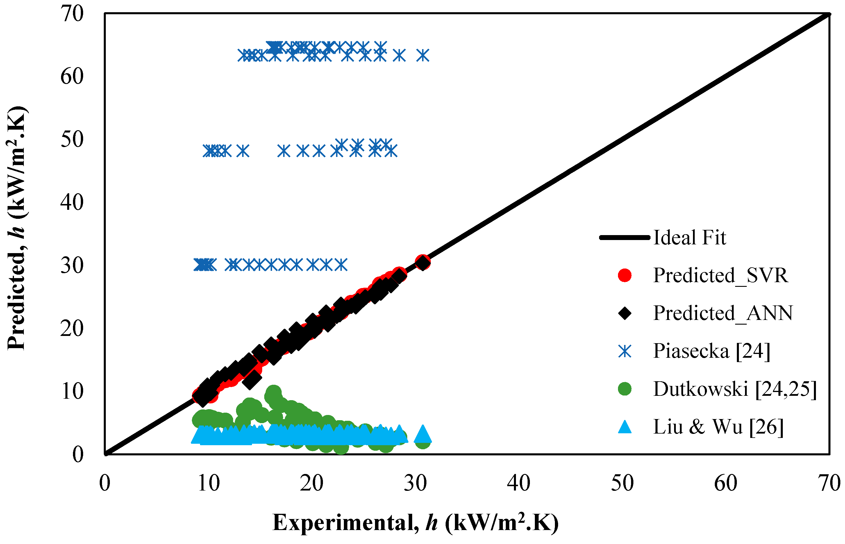
5.3. Comparative Study

This section presents a comparative study of the developed AI-based models with the existing correlations for the prediction of heat transfer coefficient of R600a in mini-channels.

Table 5. Evaluation of the AI-based models versus existing correlations over the test dataset.

Correlations	Model Evaluation Indices
	AARE (%)	R2	RMSE	SD	MRE	MAE (%)
SVR (Present study)	1.15	0.9981	0.2365	4.8343	0.0115	0.28
ANN (Present study)	5.14	0.9685	0.8608	5.2438	0.0514	1.05
Piasecka [24]	62.52	0.1600	35.61	14.0801	6.252	33.2313
Dutkowski [24,25]	43.89	0.2624	15.32	12.2	4.3893	13.68
Li and Wu [26]	47.68	0.0095	16.19	17.78	4.76	18.35

shows the performances of AI-based models and the existing correlations in terms of statistical measures over the test dataset (unseen data). A small average absolute relative error (1.15%), root mean square error (0.2365), and high R² value (0.9981) suggest that the SVR-based model has highly improved statistical parameters in comparison to the other models. In Figure 6, all the predicted data points of the SVR model lie close to the ideal fit line while the predicted data points found using the ANN model lie slightly away from the ideal fit line. Thus, the obtained results in Table 5 and Figure 6 reveal the superior predictability of the SVR-based model. The SRM of the SVR model exhibits superior prediction performance as it optimizes the generalization accuracy around the empirical error and the flatness of the model or the capacity of SVM. While the ERM of the ANN minimizes the empirical error (error associated with the training data) and does not consider the capacity of the learning machines. This results in overtraining, i.e., high accuracy for the training dataset and low for test data, giving poor generalization performance [12,20]. Furthermore, none of the existing correlations (namely Piasecka [24], Dutkowski [24,25], and Li and Wu [26]) predict the heat transfer coefficient of R600a accurately. This might be due to the fact that these correlations have been developed for different refrigerants with different flow conditions.

Table 6. Percentage of predicted data points for the heat transfer coefficient of R600a via the ANN-based and SVR-based model in terms of absolute deviation (AD) for the training dataset.

Absolute Deviation (AD) (%)	% of ANN Model Predicted Values	Cumulative Score	% of SVR Model Predicted Values	Cumulative Score
AD < 5	61.96	61.96	93.73	93.73
5 < AD < 10	23.53	85.49	5.09	98.82
AD > 10	14.51	100	1.18	100
Total	100		100

illustrates the distribution of the predicted data points of the heat transfer coefficient of R600a based on ANN-based and SVR-based models in terms of the absolute deviation (AD) for the training dataset. 61.96% of predicted data points via ANN model are observed nearly within an AD of less than 5%. 23.53% of predicted data points are between an absolute deviation of 5 and 10%, and 14.51% of predicted data points are above an AD of 10%. Now, in the SVR-based model, 98.82% predicted data points lie below an AD of 10%, and only 1.18% predicted data points are above an AD of 10%.

Table 7. Percentage of predicted data points for the heat transfer coefficient of R600a via the ANN-based and SVR-based model in terms of absolute deviation for test (unseen) dataset.

Absolute Deviation (AD) (%)	% of ANN Model Predicted Values	Cumulative Score	% of SVR Model Predicted Values	Cumulative Score
AD < 5	68.75	68.75	96.88	96.88
5 < AD < 10	28.12	96.87	3.12	100
AD > 10	3.13	100	0.00
Total	100		100

summarizes the distribution of predicted data points of heat transfer coefficient of R600a based on ANN-based and SVR-based models in terms of the absolute deviation for the test dataset. 68.75% of predicted data points via the ANN model are within an absolute deviation of less than 5%. 28.12% of predicted data points are in between an absolute deviation of 5% and 10%, 96.87% data points lie below an absolute deviation of 10%, and 54.55% data points are above an AD of 10%. The SVR-based model predicts nearly 96.88% of data points, having less than 5% absolute deviation, and all the data points falls within an absolute deviation of not more than 10%.

5.4. Parametric Study

The following section discusses the performance of AI-based models for predicting the effects of input parameters, namely heat flux (q), vapor quality (x), mass flux (G), and saturation temperature (T_sat) on the heat transfer coefficient (h) of R600a in a mini-channel.

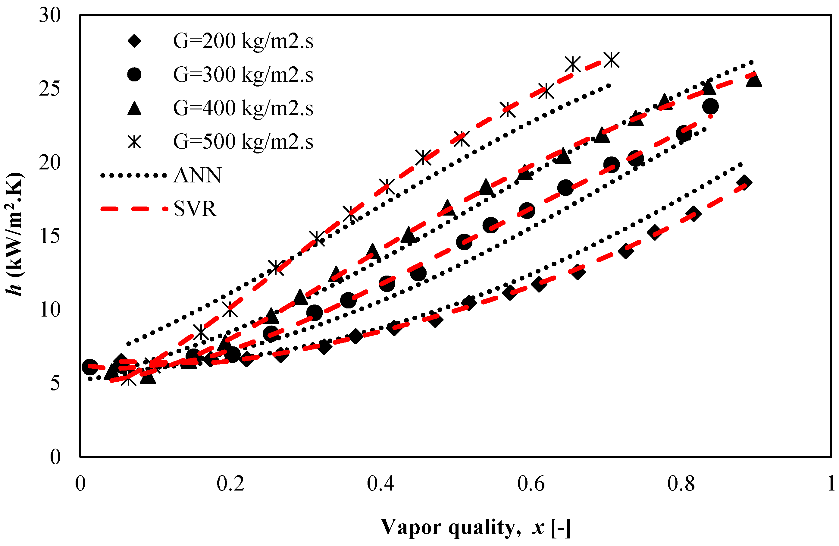
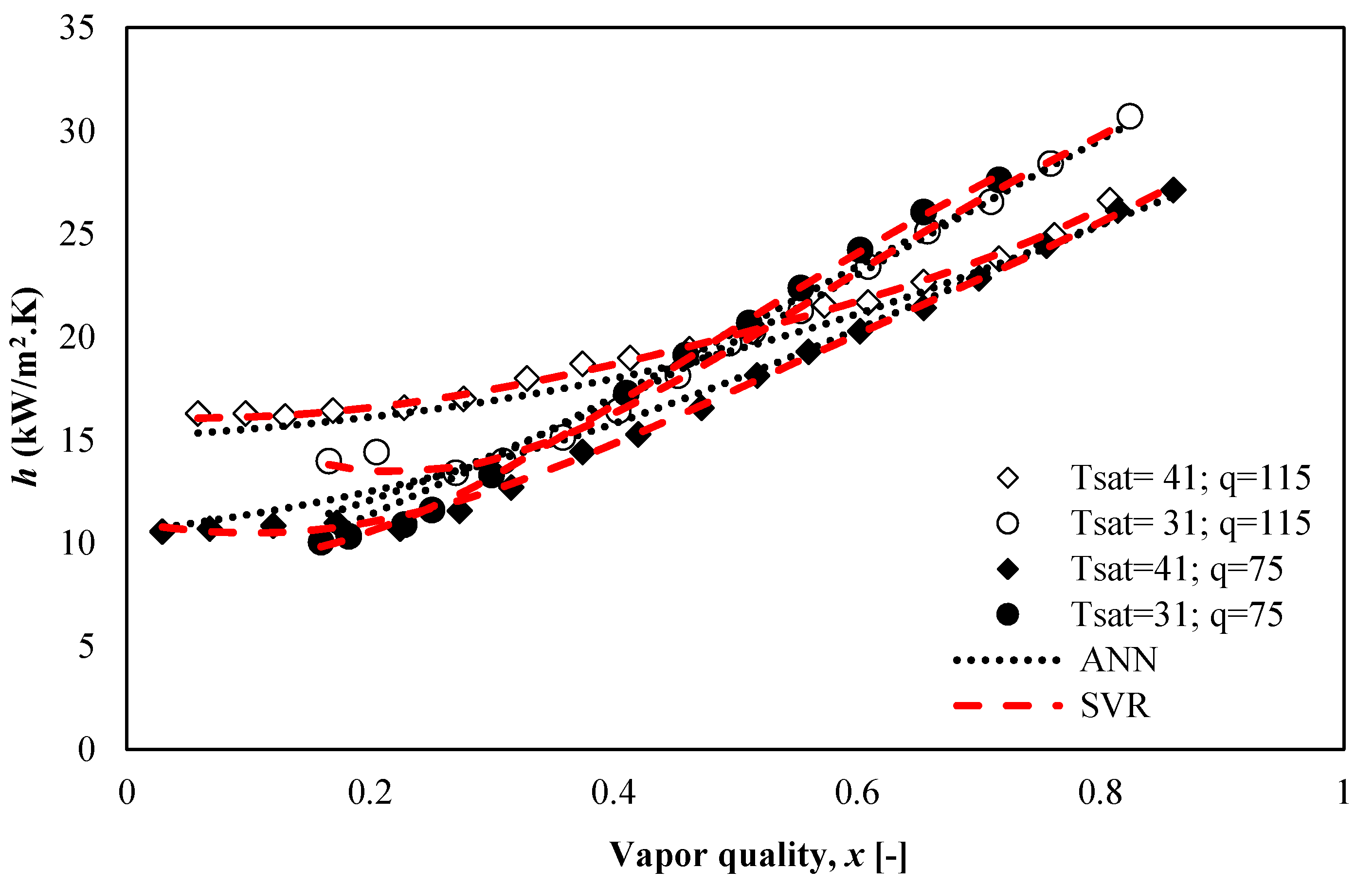
5.4.1. Effect of Heat Flux and Vapor Quality on the Heat Transfer Coefficient of R600a

Figure 7 is a plot of vapor quality versus the heat transfer coefficient of R600a for various heat fluxes at a constant mass flux (400 kg/m²·s) and saturation temperature (41 °C). It depicts the increase of the heat transfer coefficient with the increase of heat flux at low and intermediate vapor qualities. However, at high vapor qualities heat flux does not have much influence over the heat transfer coefficient. This implies the nucleate boiling dominant region at high heat flux levels and low vapor qualities [27,30]. The simulated results from ANN-based and SVR-based models follow the same trend as that of experimental results. Moreover, the predicted results from the ANN-based model slightly deviate from the observed values because of the ERM principle on which ANN is based upon.

5.4.2. Effect of Mass Flux on the Heat Transfer Coefficient, h of R600a

Figure 8 demonstrates the effect of mass flux (kg/m²·s) on the heat transfer coefficient for R600a at a constant heat flux (45 kW/m²) and saturation temperature (31 °C). This figure clearly shows that the heat transfer coefficient increases with increasing mass flux at intermediate and high vapor qualities as convective boiling occurs. At low vapor qualities, the nucleate boiling dominates and the heat transfer coefficient was found to be almost independent of mass flux [27].The modeled heat transfer coefficient is found to have been a sound match with the experimental results. In fact, the SVR-based model has excellent prediction performance due to its SRM principle.

5.4.3. Effect of Saturation Temperature on the Heat Transfer Coefficient of R600a

Figure 9 demonstrates the observed and modeled heat transfer coefficient for R600a at two different values of T_sat (i.e., 31 and 41 °C) and heat fluxes (115 and 75 kW/m²) with a constant mass flux (500 Kg/m²·s). At low vapor qualities, the heat transfer coefficient increases with increasing saturation temperature. However, at high vapor qualities, an opposite trend occurs. This change of behavior is mainly because of a decrease in heat flux [27]. Furthermore, the SVR-based model most accurately predicts the heat transfer coefficient, followed by the ANN-based model.

6. Conclusions

AI-based models have been built to predict the heat transfer coefficient of R600a in a mini-channel. The simulated results obtained were in good agreement with the experimental results. Moreover, based on the statistical measures, training and test course curve, and the AD value, the predictability of the SVR-based model outperforms the ANN model and the existing correlations. Neither of the existing correlations, namely Piasecka [24], Dutkowski [24,25], and Li and Wu [26], provide an accurate prediction of the heat transfer coefficient of R600a. This is because these correlations have been developed for different refrigerants which have different flow conditions. Moreover, parametric studies clearly depict the excellent prediction performance of the SVR model, which is attributed to the fact that it is based on an SRM principle. This optimizes the generalization accuracy over the empirical error and the model complexity or the capacity of the machines. Good SVR prediction results can be helpful in the more efficient design and fabrication of heat transfer equipment, and it appears to be a promising technique for the prediction in micro- or mini-channels. Thus, the SVR method, as an artificial intelligence technique, can be applied in chemical engineering and its allied fields.

References

1. Kandlikar, S.G. Fundamental issues related to flow boiling in minichannels and microchannels. Exp. Therm. Fluid Sci. 2002, 26, 389–407. [Google Scholar] [CrossRef] [Green Version]
2. Rao, M.; Khandekar, S. Simultaneously Developing Flows Under Conjugated Conditions in a Mini-Channel Array: Liquid Crystal Thermography and Computational. Heat Transf. Eng. 2009, 30, 751–761. [Google Scholar] [CrossRef]
3. Copetti, J.B.; Macagnan, M.H.; Zinani, F. Experimental study on R-600a boiling in 2.6 mm tube. Int. J. Refrig. 2013, 36, 325–334. [Google Scholar] [CrossRef]
4. Choi, K.I.; Oh, J.T.; Saito, K.; Jeong, J.S. Comparison of heat transfer coefficient during evaporation of natural refrigerants and R-1234yf in horizontal small tube. Int. J. Refrig. 2014, 41, 210–218. [Google Scholar] [CrossRef]
5. de Oliveira, J.D.; Copett, J.B.; Passos, J.C. An experimental investigation on flow boiling heat transfer of R-600a in a horizontal small tube. Int. J. Refrig. 2016, 72, 97–110. [Google Scholar] [CrossRef]
6. Smola, A.J.; Schölkopf, B. A tutorial on support vector regression. Stat. Comput. 2004, 14, 199–222. [Google Scholar] [CrossRef] [Green Version]
7. Zaidi, S. Development of support vector regression (SVR)-based model for prediction of circulation rate in a vertical tube thermosiphon reboiler. Chem. Eng. Sci. 2012, 69, 514–521. [Google Scholar] [CrossRef]
8. Parveen, N.; Zaidi, S.; Danish, M. Support Vector Regression Prediction and Analysis of the Copper (II) Biosorption Efficiency. Indian Chem. Eng. 2017, 59, 295–311. [Google Scholar] [CrossRef]
9. Akande, K.O.; Owolabi, T.O.; Olatunji, S.O.; Raheem, A.A.A. A hybrid particle swarm optimization and support vector regression model for modelling permeability prediction of hydrocarbon reservoir. J. Pet. Sci. Eng. 2017, 150, 43–53. [Google Scholar] [CrossRef]
10. Santamaría-Bonfil, G.; Reyes-Ballesteros, A.; Gershenson, C. Wind speed forecasting for wind farms: A method based on support vector regression. Renew. Energy 2016, 85, 790–809. [Google Scholar] [CrossRef]
11. Moazami, S.; Noori, R.; Amiri, B.J.; Yeganeh, B.; Partani, S.; Safavi, S. Reliable prediction of carbon monoxide using developed support vector machine. Atmos. Pollut. Res. 2016, 7, 412–418. [Google Scholar] [CrossRef]
12. Zaidi, S. Novel application of Support Vector Machines to model the two phase-boiling heat transfer coefficient in a vertical tube thermosiphon reboiler. Chem. Eng. Res. Des. 2015, 98, 44–58. [Google Scholar] [CrossRef]
13. Parveen, N.; Zaidi, S.; Danish, M. Support vector regression model for predicting the sorption capacity of lead (II). Perspect. Sci. 2016, 8, 629–631. [Google Scholar] [CrossRef]
14. Parveen, N.; Zaidi, S.; Danish, M. Development of SVR-based model and comparative analysis with MLR and ANN models for predicting the sorption capacity of Cr(VI). Process Saf. Environ. Prot. 2017, 107, 428–437. [Google Scholar] [CrossRef]
15. Yunos, Y.M.; Rosli, M.A.; Ghazali, N.M.; Pamitran, A.S. Performance of natural refrigerants in two phase flow. J. Teknol. Sci. Eng. 2016, 78, 77–83. [Google Scholar]
16. Kim, M.; Lim, B.; Chu, E. The Performance Analysis of a Hydrocarbon Refrigerant R-600a in a Household Refrigerator/Freezer. KSME Int. J. 1998, 12, 753–760. [Google Scholar] [CrossRef]
17. Vapnik, V.N. An overview of statistical learning theory. IEEE Trans. Neural Netw. 1999, 10, 988–999. [Google Scholar] [CrossRef] [PubMed]
18. Gunn, S. Support Vector Machines for Classification and Regression; ISIS Technical Report; University of Southampton: Southampton, UK, 1997; pp. 1–42. [Google Scholar]
19. Hearst, M.A.; Dumais, S.T.; Osman, E.; Platt, J.; Scholkopf, B. Support vector machines. IEEE Intell. Syst. 1998, 13, 18–28. [Google Scholar] [CrossRef]
20. Vapnik, V.; Golowich, S.E.; Smola, A. Support Vector Method for Function Approximation, Regression Estimation, and Signal Processing. Adv. Neural Inf. Process. Syst. 1996, 9, 281–287. [Google Scholar]
21. Sibi, P.; Jones, S.; Siddarth, P. Analysis of different activation functions using back propagation neural networks. J. Theor. Appl. Inf. Technol. 2013, 47, 1264–1268. [Google Scholar]
22. Devabhaktuni, V.; Yagoub, M.; Fang, Y.; Xu, J.; Zhang, Q.-J. Neural networks for microwave modeling: Model development issues and nonlinear modeling techniques. Int. J. RF Microw. Comput. Eng. 2001, 11, 4–21. [Google Scholar] [CrossRef]
23. Kung, C.; Yang, W.; Kung, C. A Study on Image Quality Assessment using Neural Networks and Structure Similarty. J. Comput. 2011, 6, 2221–2228. [Google Scholar] [CrossRef]
24. Sempértegui-Tapia, D.F.; Ribatski, G. Flow boiling heat transfer of R134a and low GWP refrigerants in a horizontal micro-scale channel. Int. J. Heat Mass Transf. 2017, 108, 2417–2432. [Google Scholar] [CrossRef]
25. Sherrod, P.H. DTREG: Predictive Modeling Software; DTREG: Brentwood, TN, USA, 2013. [Google Scholar]
26. Peng, H.; Ling, X. Predicting thermal-hydraulic performances in compact heat exchangers by support vector regression. Int. J. Heat Mass Transf. 2015, 84, 203–213. [Google Scholar] [CrossRef]
27. Piasecka, M. Correlation for flow boiling heat transfer in minichannels with various orientations. Int. J. Heat Mass Transf. 2015, 81, 114–121. [Google Scholar] [CrossRef]
28. Dutkowski, K. Heat Transfer and Pressure Drop during Single-Phase and Two-Phase Flow in Minichannels (in Polish), Monograph; The Publishing House of Kozalin University of Technology: Kozalin, Poland, 2011. [Google Scholar]
29. Li, W.; Wu, Z. A general correlation for evaporative heat transfer in micro/mini-channels. Int. J. Heat Mass Transf. 2010, 53, 1778–1787. [Google Scholar] [CrossRef]
30. Bertsch, S.S.; Groll, E.A.; Garimella, S.V. Effects of heat flux, mass flux, vapor quality, and saturation temperature on flow boiling heat transfer in microchannels. Int. J. Multiph. Flow 2009, 35, 142–154. [Google Scholar] [CrossRef] [Green Version]
Figure 1. The schematic topology of the 4:7:1 ANN architecture.
Chemengineering 02 00027 g001
Figure 2. (a) Training course curve for the heat transfer coefficient. (b) Test course curve for the heat transfer coefficient.
Chemengineering 02 00027 g002
Figure 3. ANN model performance assessment using the training and test dataset.
Chemengineering 02 00027 g003
Figure 4. (a) Training course curve for the heat transfer coefficient. (b) Test course curve for the heat transfer coefficient.
Chemengineering 02 00027 g004
Figure 5. SVR simulation of heat transfer coefficient of R600a using the optimal parameters.
Chemengineering 02 00027 g005
Figure 6. Performance comparison of AI-based models versus existing correlations for predicting the heat transfer coefficient on the test dataset.
Chemengineering 02 00027 g006
Figure 7. Observed and modeled heat transfer coefficient for R600a in a mini-channel at different heat fluxes (G = 400 kg/m2·s; Tsat = 41 °C).
Chemengineering 02 00027 g007
Figure 8. Observed and modeled heat transfer coefficient for R600a in a mini-channel at different mass fluxes (q = 45 kW/m2; Tsat = 31 °C).
Chemengineering 02 00027 g008
Figure 9. Observed and modeled heat transfer coefficient for R600a in a mini-channel at two different saturation temperatures in °C (q = 115 kW/m2 and 75 kW/m2; G = 500 kg/m2·s).
Chemengineering 02 00027 g009