Optimization of Chemical Processes by the Hydrodynamic Simulation Method (HSM)

Abstract

We describe a hydrodynamic simulation method (HSM) that is based on hydrodynamic considerations in Batch and Semi Batch stirred reactor systems. The method combines hydrodynamic studies of the mixing procedure obtained from experiments in small and large scale stirred reactors together with process simulation by VisiMix software. We describe how this hydrodynamic simulation method can aid in process optimization and scale up. The use of the simulation method described in this article, will offer the user the possibility to achieve the best results during production stage, saving time and currency, and at the same time increasing the knowledge of the performed process. Several examples in the article demonstrate the benefits of the proposed method.

1. Introduction

Chemical production is based on chemical reactions, purification steps, and product characterization [1]. Understanding the reaction system has a critical impact on the yields of each step since the total yield of the crude product has a great impact on the purification step and hence on the final product quality and cost [2,3].

Chemical reactions in the industries are frequently performed in stirred reactors that are operated at batch, semi-batch, or continuous flow configuration [4]. The choice of the operation configuration is done in the planning stages of the process development. However, if the chemistry of the reaction and its hydrodynamics are not well understood, wrong selection of conditions will be adopted in the process development [5,6].

According to some sources, the estimated amount of currency that can be saved by optimizing a process of a blockbuster drug on the market is approximately 500 million US dollars. And the estimated loss resulted from un-optimized hydrodynamics is approximately 1 to 10 billion dollars in the US chemical industry alone [5].

Scale up and transfer of technical activities are expansive, risky stages. This is due to the use of different equipment that has geometrical differences leading to differences in mass and heat transfer [7,8]. Obviously, scale up activities performed in large reactors involve high cost because large quantities of solvents and materials are used in the process [6]. If, for some reason, it is impossible to manufacture a product with high yield and good quality, the consequences could be a failure in the operation. Since the raw materials and the chemical production procedures at this stage are not about to change, the main reason for the failure arise from the selection of inappropriate equipment and process operation protocol [9]. The operation conditions are mainly governed by the mixing operation, and thus by controlling mixing it is possible to improve the operation [6]. Good mixing is considered as the capability to provide conditions to the process that generate appropriate operation, that results in high yield and quality at every step of the production process. Identification of the mixing and hydrodynamic parameters will provide the knowledge to dramatically reduce the uncertainty in process development [4].

Once a process is well known, not only from the chemical aspect, but also from the hydrodynamic aspect (e.g., heat, mass, and momentum transfer), only then is it possible to design an optimal process for production. The reason is that the yields of some diffusion controlled reactions are highly depended on the hydrodynamic properties. For example, semi-batch reactions and multiphase reactions are process that are diffusion dependent [1,5,9]. There is a common issue in production yields when transferring a process to a different location or scale it up [5,6,9,10]. Since large scale processes highly depend on the hydrodynamics, controlling it will decrease the effect of the changes in scale or location on the yields of the process [5,11]. Simulations and calculations of hydrodynamics parameters can dramatically increase the efficiency of the process and hence decrease the process development time, resulting in a better optimization course [5].

In this paper, we will describe a hydrodynamic simulation method (HSM) for the simulation of the effect of mixing and hydrodynamics on the process parameters, and describe how the control of mixing parameters can be used for evaluation of chemical processes.

2. Materials and Methods

2.1. Scale-Down Scale-Up (SDSU) Methodology in Process Development

The SDSU concept is used to collect crucial hydrodynamic data from bench scale equipment. The data exploited by mathematical and computational methods [12]. Thus, scale-down is used to characterize the process in small scales giving information on the hydrodynamic and chemical properties, resulting in better understanding of the system. When a process is fully characterized, simulation can be used for scale up to a pilot step in the chemical industries. The simulation keeps many crucial hydrodynamic parameters in control, thus saving time in the design of a pilot and producing a more optimized process [13].

After few loops of bench scale experiments and suitable calculations it will be possible to scale up the designed plant to pilot plant facilities and confirm the hybrid model-experimental data at plant facilities conditions. After the last critical step it will be possible to perform fine-tuning and design the large scale production process.

When the SDSU methodology is used, recognition of the important elements allows more efficient simulation. The important elements are: chemical mechanism, first class analytical follow up methods, reaction feasibility, correct equipment for practical and theoretical simulation of the reaction and an ability to verify the data.

VisiMix process simulation tool is in use by more than 200 companies for process optimization. The superiority of this tool demonstrated in variety of case studies [5,14]. The high accuracy of these simulations produced reliable alternative to pilot experiments.

2.2. The Use of the Hydrodynamic Simulations Method for Process Development and Optimization

When the parameters of the reaction and reactor are known, they can be fed into VisiMix simulation program to estimate the hydrodynamic parameters. The program gives us as output the characteristics of the hydrodynamics during the reaction. VisiMix program can estimate the parameters of Hydrodynamic Turbulence Single Liquid Phase (HT-SLP) with high accuracy. The simulated data input into trail experiments and tested, after few trail experiment the process is ready for high scale production [15,16,17,18].

Hydrodynamics is a sub discipline of fluid mechanics that describes the flow of fluids and deals with the motion of fluids and the interaction forces with the solid environment. The motion of the fluids generates turbulent flow that plays key role in the momentum, heat and mass transfer during the operation of the reactor. Motion of fluids in a stirred reactor is provided by the rotation of an impeller, this source of motion in fluids also known as mixing [19]. There are crucial mixing parameters in different type of reaction and they can be calculated by VisiMix simulation tool [20]. The key parameters for each type of process are shown in

Table 1. Mixing Key Parameters for Different Applications [5].

Application	Key Process and Scale-Down Scale-Up Parameters
Newtonian Non Newtonian Hydrodynamics and Scale-up	Circulation flow rate
	Local values of energy dissipation
	Turbulent Shear rates
Blending-Single Phase mixing	Macro and micro mixing times
	Max./Min. concentration difference ΔC
Liquid-Solid Suspension, Crystallization, Dissolution	Max. local concentrations
	Max. shear rate
	Crystal collision energy
Liquid-Liquid Emulsification, Heterogeneous Synthesis	Drop size distribution
	Specific mass transfer area
	Micro mixing time for disperse phase
Liquid-Gas Gas injection, Absorption, Gas Liquid Reactors	Gas hold up
	Specific mass transfer area
	Specific mass transfer coefficient
Biotechnology	Oxygen mass transfer rate
Heat Transfer in Vessels with Different Heating/Cooling Devices	Media temperature
	Heat transfer coefficient
	Specific heat/cool rate

.

VisiMix simulation tool gives us important parameters that should be always taken into consideration such as: Mixing power that has different limits in different equipment and the user should be aware of equipment limits; Reynolds Number (Re) characterizes the turbulent or laminar flow regime based on average flow and reactor size; Vortex Parameters which have impact on media near the reactor walls and affect the heat and mass transfer; Gas pick-up from the surface that can cause the formation of gas bubbles in the liquid; Circulation flow rate that indicate the average time for media circulation in the reactor, this parameter is especially crucial in semi batch reactor with pipe inlet; Dissipation energy is the energy distribution in different zones of reactor, this parameter is crucial for process such as micro mixing, crystallization and emulsification; Turbulent shear rates is a micro scale characteristic of shear rate that affects dissolution rate of solid particles; and mixing time that indicates the time to form a homogenous solution with uniform distribution of substances. The simulation not only calculates important parameters but can also visualize the flow pattern in the reaction vessel.

When all the parameters are known, it is possible to design a trail experiment for additional data collection, which will result in easy and convenient scale up process.

3. Results

The following examples were performed by different VisiMix users from several companies:

3.1. Example 1: Single-Phase Flow

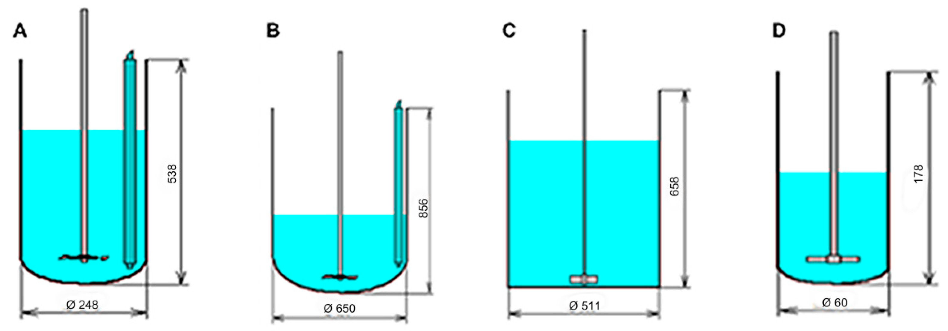
This study shows a comparison of mixing between four types of reactors for semi batch processes. And the task is to identify the differences between the mixing parameters in each reactor. The parameters of each reactor are shown in Figure 1.

The parameters simulated with additional standard consideration of density = 1000 kg/m³ and viscosity of 1 cP. The simulation data is shown in

Table 2. Full data for simulation of all the reactors.

General Hydrodynamics Main Characteristics
Parameter	Unit	Reactor A	Reactor B	Reactor C	Reactor D
Rotation Speed	rpm	45	45	200	500
Mixing Power	W	0.00224	0.0289	0.419	0.00712
Reynolds for Flow	----	3610	19800	42300	6470
Tangential Velocity (Average)	m/s	0.0241	0.0611	0.165	0.215
Circulation Flow Rate	m3/s	0.00042	0.000109	7.46 × 10−5	6.44 × 10−6
Circulation Velocity (Average)	m/s	0.0164	0.000616	0.000364	0.00226
Turbulence Main Characteristics
Rotation Speed	rpm	45	45	200	500
Energy Dissipation, Maximum	W	0.0192	0.0306	8.14	8.97
Energy Dissipation, Average	W	0.000134	0.00029	0.00419	0.0285
Energy Dissipation, Bulk Volume	W	9.4 × 10−5	0.00021	0.00161	0.0123
Turbulent Shear Rate Near Impeller	1/s	139	175	2860	3000
Turbulent Shear Rate in Bulk Volume	1/s	9.74	14.5	40.3	111
Single-Phase Mixing. Main Characteristics
Rotation Speed	rpm	45	45	200	500
Macro Mixing Time	s	102	122	198	27.2
Mean period of circulation	s	39.8	921	1340	38.8
Micro Mixing Time	s	103	69	24.9	9.02

.

As expected, the main parameter characteristics of mixing of the four reactors are very different.

As a general rule, for a semi batch chemical reaction process, it is recommended that the Mean Period of Circulation should be as small as possible and the shear rate at the point of feeding is as high as possible. Under these considerations, the reactors that seem to be more suitable for this case are reactors A and D.

3.2. Example 2: Two Phase Flow without Chemical Reaction

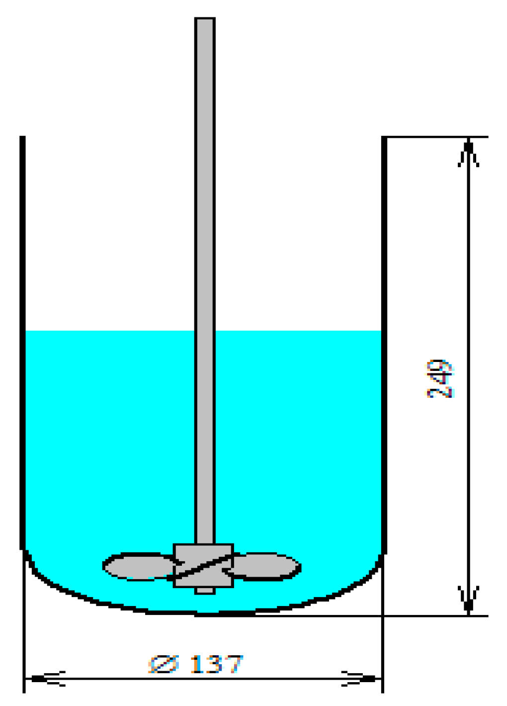
This case shows the importance of mixing in bioreactors with a combination of liquid-solid and liquid-gas two-phase processes in water. The task is to study the process in the bioreactor and improve the gas and solid distribution inside the bioreactor with 10 micron size particles in 200 kg/m³ concentration. The parameters of the bioreactor shown in Figure 2.

Simulation performed with these parameters giving the hydrodynamic parameters that should be constant in the scale up process. The parameters are shown in

Table 3. Hydrodynamic parameters in the bioreactor.

Parameter	Units	Value
General Basic Parameters
Circulation flow rate	m3/s	2.39 × 10−5
Energy dissipation in the bulk of volume	W/kg	0.00506
Microscale of turbulence in the bulk of volume	m	0.000119
Liquid-Solid Mixing
Complete suspension expected	----	YES
Maximum degree of non-uniformity-Axial	%	15.6
Maximum degree of non-uniformity-Radial	%	57.4
Maximum local concentration of solids	kg/m3	247
Minimum local concentration of solids	kg/m3	73.2

.

Suitability of the equipment to gas dispersion processes and its efficiency depend on the possibility for the complete dispersion of the gas entered under the agitator and on the distribution of the bubbles in the tank volume. Because of this condition simulation is not possible and calculations for scale-up/down have to be done by approach to General Basic Parameters, the impeller rotation increased to 270 to increase axial circulation rate. The parameters that were simulated in these conditions are shown in

Table 4. Hydrodynamic parameters in the bioreactor after changing the conditions.

Parameter	Units	Value
General Basic Parameters
Circulation flow rate	m3/s	0.00108
Energy dissipation in the bulk of volume	W/kg	0.0217
Microscale of turbulence in the bulk of volume	m	8.24 × 10−5
Liquid-Solid Mixing
Complete suspension expected	----	YES
Maximum degree of non-uniformity-Axial	%	4.27
Maximum degree of non-uniformity-Radial	%	0.166
Maximum local concentration of solids	kg/m3	209
Minimum local concentration of solids	kg/m3	191
Gas Dispersion and Mass Transfer
Gas distribution	-----	Satisfactory
Gas hold-up	-----	0.000247
Sauter mean bubble diameter	m	0.00197
Estimated surface aeration rate	m/s	0
Specific mass transfer area	m2	0.754
Specific mass transfer coefficient	1/s	0.000228
Gas mass transfer rate	kg/h	6.56 × 10−5

.

3.3. Example 3: Two-Phase Flow with Chemical Reaction

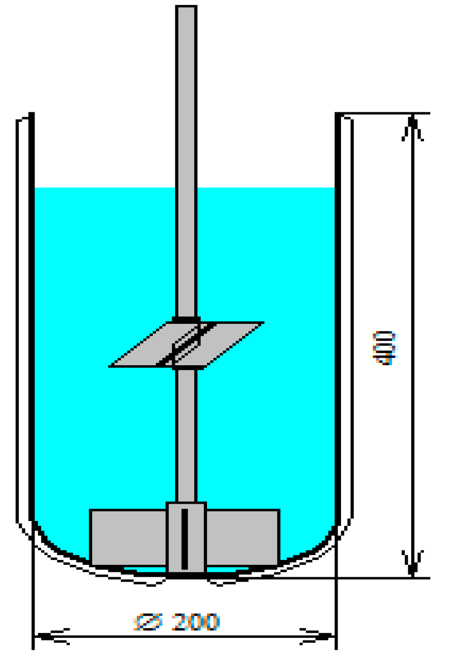
The case in this example is a chemical reaction which occurring in continuous flow within heterogeneous liquid-solid system. The problem is as follows: Solid raw materials A and B dissolved in solvent C (A + B is 70 wt% total) at 80 °C, and heated to 145 °C for 11 h for full conversion to product D. After 1.5 h the product D is starting to crystallize. The system at the end of the reaction is a heterogeneous system with 30% of the solvent C and 70% of the solid D. the task is to determine the characteristic parameters of the process during mixing for the purpose of satisfactory scale up. The known parameters of the reactions are the average density of the solution which is 1100 kg/m³ and the dynamic viscosity which is around 5 cP. Also the parameters of the vessel used are known. The inlet tubing radius: 9.7 mm, the height from bottom: 450 mm and the volume flow rate: 1 × 10⁻⁶ m³/s. The outlet height from bottom is 100 mm. And reactor parameters as shown in Figure 3.

Simulation by the VisiMix program showed that the main contributor to the mixing is the bottom impeller. And the circulation flow rate is 0.00167 m³/s which is much higher than the volume flow rate. This means that the volume flow rate is irrelevant. From these results we learn that we can do the simulation by only using the bottom impeller in turbulent flow.

Continuous flow dynamics used with mathematical simulation of the stimulus-response testing technique which is generally used to evaluate the reactor deviation from ideal. The testing method is based on tracing the reactor with a tracer, usually with a radioactive isotope solution. The tracer is injected in the reactor (“pulse-mode input”), and the response function curve is obtained by measuring the tracer’s concentration at the outlet of the vessel.

The response functions for different inlet and outlet positions can be calculated. The deviation of the actual residence distribution (RTD) can be calculated from RTD in an ideal (“perfect mixing”) reactor of the same volume.

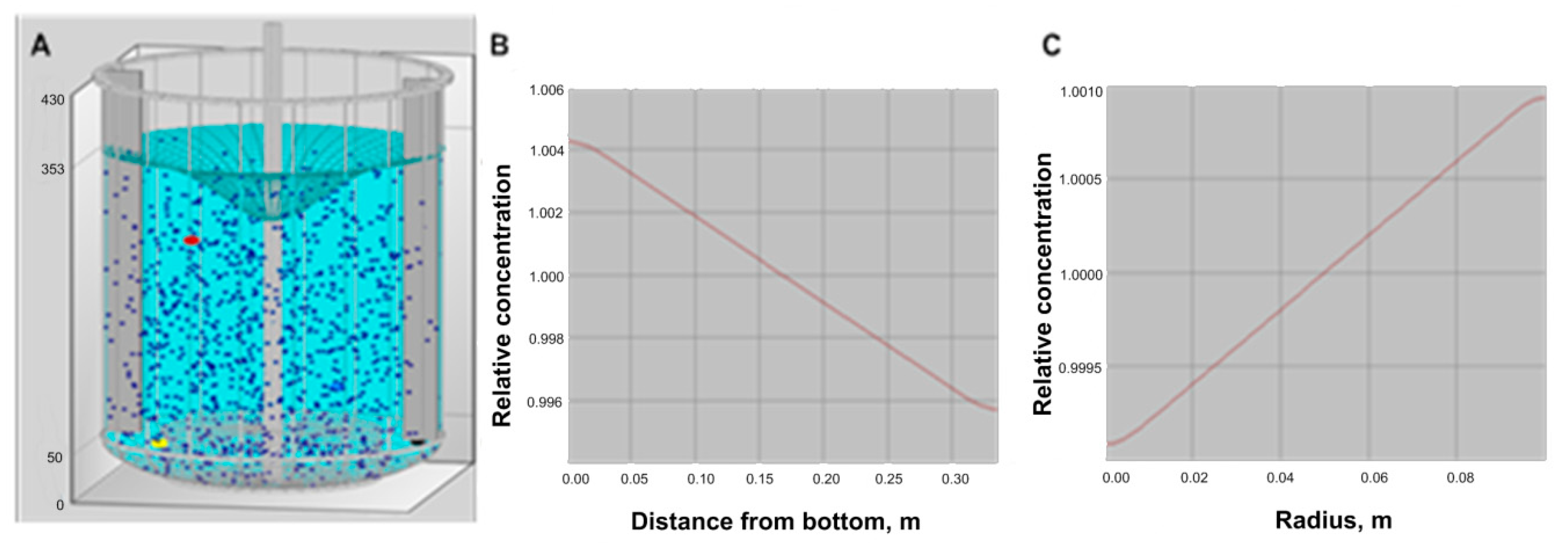
Liquid-Solid Mixing: Use this option to calculate the mixing of suspensions. The modeling of the solid phase distribution is based on a diffusion model of turbulent transport in quasi-homogeneous media. Separation under the effect of the rotation flow and practical data on the pick-up of particles from the bottom is also taken into account. Solid distribution is adequate as shown in Figure 4, but because of vortex, high solid concentration, and particles sizes, complete solid suspension is questionable, and could affect the crystallization result.

For solid suspension it is recommended to use a reactor with baffles. Simulation with the addition of two baffles to the system is described in Figure 5. By adding the baffles the vortex is reduced resulting in better solid distribution especially the radial distribution.

4. Conclusions

The VisiMix simulation program allows us to calculate the main hydrodynamics parameters of a reaction. By reaching similar values at any scale it is possible to achieve the optimal solution of the mixing process. In these conditions, one can understand better the processes, reduce dramatically the time and cost of the SDSU processes, and save a huge amount of time & currency. The simulations yield quick results, based on a systematic and serious evaluated experimental data collection. In addition, the simulations were found as very reliable and accurate sources for hydrodynamic parameters in chemical processes.

References

- Levenspiel, O. Chemical reaction engineering. Ind. Eng. Chem. Res. 1999, 38, 4140–4143. [Google Scholar] [CrossRef]
- Faure, A.; York, P.; Rowe, R.C. Process control and scale-up of pharmaceutical wet granulation processes: A review. Eur. J. Pharm. Biopharm. 2001, 52, 269–277. [Google Scholar] [CrossRef]
- Schmidt, F.R. Optimization and scale up of industrial fermentation processes. Appl. Microbiol. Biotechnol. 2005, 68, 425–435. [Google Scholar] [CrossRef] [PubMed]
- Kunii, D.; Levenspiel, O. Fluidization Engineering; Howard Brenner: New York City, NY, USA, 1991; ISBN 9780409902334. [Google Scholar]
- Bentolila, M.; Novoa, R. Scale up Methodology for the Fine Chemical Industry—The Influence of the Mixing in the Process; VISIMIX Ltd.: Jerusalem, Israel, 2011. [Google Scholar]
- Harnby, N.; Edwards, M.F.; Nienow, A.W. Mixing in the Process Industries; Butterworth-Heinemann: Oxford, UK, 1997; ISBN 9780080536583. [Google Scholar]
- Holman, J. Heat Transfer; Mc Graw Hill: New York City, NY, USA, 2010. [Google Scholar]
- Dutta, B.K. Principles of mass transfer and separation processes. Can. J. Chem. Eng. 2009, 87, 818–819. [Google Scholar] [CrossRef]
- Paul, E.L.; Kresta, S.M. Handbook of Industrial Mixing; John Wiley & Sons: Hoboken, NJ, USA, 2004. [Google Scholar] [CrossRef]
- Ng, K.M.; Wibowo, C. Beyond process design: The emergence of a process development focus. Korean J. Chem. Eng. 2003, 20, 791–798. [Google Scholar] [CrossRef]
- Mah, R.S.H. Chemical Process Structures and Information Flows; Butterworths: Oxford, UK, 1990; ISBN 9781483278339. [Google Scholar]
- Berty, J.M. Changing Role of the Pilot Plant. Chem. Eng. Prog. 1979, 75, 48–51. [Google Scholar]
- Basu, P.K.; Mack, R.A.; Vinson, J.M. Consider a new approach to pharmaceutical process development. Chem. Eng. Prog. 1999, 95, 82–90. [Google Scholar]
- Genck, W.; Hasson, M.; Manoff, E.; Novoa, R.; Bentolila, M. Computer aided process engineering at chemagis. Pharm. Eng. 2011, 31, 30–38. [Google Scholar]
- Braginskii, L.N.; Kokotov, Y.V.; Gordeev, L.S. Characteristics of macroscale transfer during mixing in apparatus with reflecting partitions. Teor. Osn. Khimicheskoi Teknol. 1986, 20, 375–380. [Google Scholar]
- Barabash, V.M.; Bragisnkii, L.N.; Gorbacheva, G.V. Calculating the Gad Concentration in Apparatus Equiped with Agitator. Teor. Osn. Khimicheskoi Teknol. 1988, 21, 654–660. [Google Scholar]
- Barabash, V.M.; Braginskii, L.N.; Liv’yant, R.Z.; Sadovskii, V.L. Effect of near-wall turbulance on mixing hydrodynamics. Teor. Osn. Khimicheskoi Teknol. 1986, 20, 798–804. [Google Scholar]
- Barabash, V.M.; Bragisnkii, L.N.; Kozlova, E.G. Use Mixing Apparatus for Highly Concentrated Suspensions. Teor. Osn. Khimicheskoi Teknol. 1990, 24, 63–68. [Google Scholar]
- Rane, C.V.; Ekambara, K.; Joshi, J.B.; Ramkrishna, D. Effect of impeller design and power consumption on crystal size distribution. AIChE J. 2014, 60, 3596–3613. [Google Scholar] [CrossRef]
- Visimix Review of Some Mathematical Models Used in VisiMix. Available online: http://visimix.com/wp-content/uploads/2015/11/Review-of-the-Main-Mathematical-Models.pdf (accessed on 20 November 2017).
Figure 1.
Four different reaction vessels used in the simulation. (A) Reaction vessel contains disk turbine with six blades. Diameter of the reactor is 248 mm and height is 538 mm, the disk tip diameter is 100 mm and blade length of 20 mm. the disk is located 63 mm above the bottom and rotation frequency is 45 RPM. (B) Reaction vessel contains disk turbine with six blades. Diameter of the reactor is 650 mm and height is 856 mm, the disk tip diameter is 175 mm and blade length of 45 mm. the disk is located 75 mm above the bottom and rotation frequency is 45 RPM. (C) Flat bottom reaction vessel contains paddle with two blades. Diameter of the reactor is 511 mm and height is 658 mm, the tip diameter is 102 mm. the paddle is located 25.5 mm above the bottom and rotation frequency is 200 RPM. (D) Reaction vessel contains paddle with 2 blades. Diameter of the reactor is 60 mm and height is 178 mm, the tip diameter is 30 mm and blade length of 45 mm. the paddle is located 20 mm above the bottom and rotation frequency is 500 RPM.
Figure 2.
Reaction vessel which contains one propeller type impeller. Diameter of the reactor is 137 mm and height is 249 mm, the impellers contain three blades the tip diameter is 76.2 mm. The impeller is located 25.5 mm above the bottom and rotation frequency is 200 rpm.
Figure 3.
Reaction vessel with two impellers. Diameter of the reactor is 200 mm and height is 400 mm, both impellers contain four blades the bottom impeller tip diameter is 127 mm and blade sizes of 51 mm and the top impeller tip diameter is 102 mm and blade size 44.5. The bottom impeller is 31.8 mm above the bottom and the top one is 200 mm above the bottom.
Figure 4.
Simulation for solid distribution in a reactor. (A) is the visualization of the particle distribution and the vortex, (B) is the axial distribution of the solid phase, and (C) is the radial distribution of the solid phase.
Figure 5.
Simulation for solid distribution in a reactor with addition of baffles. (A) is the visualization of the particle distribution and the vortex, (B) is the axial distribution of the solid phase, and (C) is the radial distribution of the solid phase.