Article

Modelling of Bubbly Flow Using CFD-PBM Solver in OpenFOAM: Study of Local Population Balance Models and Extended Quadrature Method of Moments Applications

1
Chemical Engineering Department, Sherbrooke University, Sherbrooke, QC J1H5N4, Canada
2
Mechanical Engineering Department, Iowa State University, Ames, IA 50011, USA
*
Author to whom correspondence should be addressed.
ChemEngineering 2018, 2(1), 8; https://doi.org/10.3390/chemengineering2010008
Submission received: 8 January 2018 / Revised: 15 February 2018 / Accepted: 22 February 2018 / Published: 27 February 2018
(This article belongs to the Special Issue Bubble Column Fluid Dynamics)

Abstract

:
In order to optimize and design new bubbly flow reactors, it is necessary to predict the bubble behavior and properties with respect to the time and location. In gas-liquid flows, it is easily observed that the bubble sizes may vary widely. The bubble size distribution is relatively sharply defined, and bubble rises are uniform in homogeneous flow; however bubbles aggregate, and large bubbles are formed rapidly in heterogeneous flow. To assist in the analysis of these systems, the volume, size and other properties of dispersed bubbles can be described mathematically by distribution functions. Therefore, a mathematical modeling tool called the Population Balance Model (PBM) is required to predict the distribution functions of the bubble motion and the variation of their properties. In the present paper, two rectangular bubble columns and a water electrolysis reactor are modeled using the open-source Computational Fluid Dynamic (CFD) package OpenFOAM. Furthermore, the Method of Classes (CM) and Quadrature-based Moments Method (QBMM) are described, implemented and compared using the developed CFD-PBM solver. These PBM tools are applied in two bubbly flow cases: bubble columns (using a Eulerian-Eulerian two-phase approach to predict the flow) and a water electrolysis reactor (using a single-phase approach to predict the flow). The numerical results are compared with measured data available in the scientific literature. It is observed that the Extended Quadrature Method of Moments (EQMOM) leads to a slight improvement in the prediction of experimental measurements and provides a continuous reconstruction of the Number Density Function (NDF), which is helpful in the modeling of gas evolution electrodes in the water electrolysis reactor.

1. Introduction

In recent years, there has been a growing interest in two-phase flows as they can be observed in various industries such as petroleum, mining, chemical and biotechnology [1,2,3,4]. In a two-phase flow, the dispersion of the particles (bubbles) in the continuous phase plays an important role in the process. One of the main challenges is to use the population balance model to predict the evolution of the number of bubbles and of their size in bubbly flow. To give an example, in order to optimize and enhance the efficiency of electrochemical reactors, the evolved bubbles should be under control, since the presence of bubbles has favorable and unfavorable effects, such as a resistive film for the electric current flow and ions supply heading to the electrode to participate in the electrode reaction. Bubbles can also play a role as a turbulence promoter and inducer of convection over the electrode surface [5,6,7,8]. The accurate description of bubble size evolution is then beneficial to formulate predictive models for design optimization.
In the literature concerning the simulation of gas-liquid systems, several authors have used a monodisperse model only accounting for a mean bubble size (Deen et al. [9]; Holzinger [10]; Friberg [11], Morud and Hjertager [12]; Ranade and Deshpande [13]; Ranade [14]; Schwarz and Turner [15]; Schwarz [16]). While these models reduce the computational cost of the numerical simulation, they are unable to predict the evolution of the bubble size distribution, limiting their applicability and reliability for industrial design purposes [17]. One of the main problems in modeling of multiphase dispersion is the prediction of bubble size distribution. Global polydisperse models, in which a spatially-varying field of bubble sizes is considered, can globally account for the polydispersity of the bubbles, in addition to the phase continuity equation. As global polydispersity models yield a non-constant bubble size, the disperse phase is global polydisperse with a locally monodispersed size distribution (Kerdouss et al. [18] and Ishii et al. [19]). However, by applying this approach, the local probability distribution of the bubble size is not considered. Detailed models using the locally polydisperse approach give more information on the secondary phase behavior (Dhanasekharan et al. [20]; Venneker et al. [21]). The most used methods of locally polydisperse models are the Method of Classes (CM) (Balakin et al. [22]; Bannari et al. [1]; Becker et al. [23]; Kumar and Ramkrishna [24]; Kumar and Ramkrishna [25]; Puel et al. [26]), Quadrature Method of Moments (QMOM) (McGraw [27]; Marchisio et al. [28]; Marchisio et al. [29]; Marchisio et al. [30]; Sanyal et al. [31]) and Direct Quadrature Method of Moments (DQMOM) (Silva and Lage [32]; Selma et al. [33]; Marchisio and Fox [34]). The method of classes, while intuitive and accurate, is computationally intensive due to the large number of classes required to finely discretize the Number Density Function (NDF) with a large number of classes. Compared with CM, the QMOM can consider a wide range of bubble sizes with a reduced number of equations for the moments of the NDF. However, in some evaporation and combustion problems (Fox et al. [35]; Yuan et al. [36]), the value of the NDF for null internal coordinates needs to be known, which is not the case if the QMOM method is used. DQMOM solves the equations for weights and abscissae directly. Shortcomings related to the conservation of moments affect the DQMOM approach since weights and abscissas are not conserved quantities (Yuan et al. [36]). In order to overcome these limitations, Yuan et al. [36] introduced the Extended Quadrature Method of Moments (EQMOM), which enables the shape of NDF to be reconstructed from a moment set using continuous kernel density functions instead of Dirac delta functions.
QMOM and EQMOM have been recently compared in the study of liquid-liquid dispersion in a stirred tank [33,37]. Li et al. [37] performed a comparison between QMOM and EQMOM in turbulent liquid-liquid dispersion, and they observed that these two methods provided similar predictions. They managed to reconstruct the droplet size distribution by using EQMOM. CM and DQMOM have been compared in bubbly flow by Selma et al. [33], as well. Their study was carried out based on two test cases, one involving a bubble column and the other a stirred tank. They reported that it is more computationally efficient to use DQMOM compared to CM even with a relatively low number of classes. A summary of some works concerning the coupling of E-E with Population Balance Model (PBM) and the comparison among PBMs are provided in Table 1 and Table 2, respectively.
In the present work, we simulate a gas-liquid flow in two rectangular bubble columns using CM, QMOM, DQMOM and EQMOM. The numerical results obtained in these two cases are used to compare the four solution methods for the PBE. The implementation of EQMOM provided by OpenQBMM [41] is coupled to a two-fluid solver in OpenFOAM to describe the bubble evolution in bubble columns. The EQMOM approach, coupled with a single-phase CFD solver in OpenFOAM, is then used to describe the evolution of the bubble phase in an electrochemical cell. This simplification, in the case of the electrochemical system, is possible because the bubble sizes of interest in this system are of the order of a micron, significantly smaller and having a lower Stokes number than in the case of the bubble column. In this case, then, a one-way coupling approach is sufficient.
The remainder of this article is organized as follows. First, the modeling approach is explained in Section 2. The numerical solution method used in the present work is summarized in Section 3. The numerical results obtained for the bubble columns and the electrochemical cell are presented in Section 4, comparing them to the experiments for validation purposes. Conclusions are drawn in Section 5.

2. Numerical Model

The governing equations of single-phase and two-phase system (two-fluid model) used in this model are shown in Table 3.

2.1. Population Balance Modeling

The evolution of the size distribution of a particle population, which may consist of solid particles, bubbles or droplets, is described studying the changes in space and time of the Number Density Function (NDF) n ( ζ ; x , t ) . Here, ζ indicates the internal coordinate representing the size of the discrete element of the disperse phase, x is the position vector in physical space and t is time.
Assuming the velocity of the disperse phase is known, the evolution of the NDF is defined by the population balance equation (Marchisio et al. [28], Marchisio and Fox [49], D. Ramkrishna [50]):
n ( ζ ; x , t ) t + x · U G n ( ζ ; x , t ) x · [ Γ x n ( ζ ; x , t ) ] + ζ · [ G ( ζ ) n ( ζ ; x , t ) ] = B ¯ a g ( ζ ; x , t ) D ¯ a g ( ζ ; x , t ) + B ¯ b r ( ζ ; x , t ) D ¯ b r ( ζ ; x , t ) + N ( ζ ; x , t ) ,
where U G is the velocity of the disperse phase, Γ is the diffusivity and G ( ζ ) the continuous rate of change in the space of internal-coordinate. The first term of Equation (1) represents accumulation; the second term describes convection; and the third diffusion in physical space. The source terms B ¯ br ( ζ ; x , t ) , B ¯ br ( ζ ; x , t ) , D ¯ ag ( ζ ; x , t ) and D ¯ ag ( ζ ; x , t ) are birth rate due to breakage, birth rate due to coalescence, death rate due to breakage and death rate due to coalescence, respectively. Finally, N ( ζ ; x , t ) is the rate of change of the NDF due to nucleation. In the present study, the NDF has the form of being length-based and G ( ζ ) is defined as growth rate.
Bubbles may nucleate when the liquid is supersaturated with gas. When the dissolved gas concentration reaches a critical value, bubbles nucleate. This critical value might be theoretically obtained from Classical Nucleation Theory (CNT) (Abraham [51]). The nucleation theory provides information about the generation of nuclei (the formation of cluster of molecules after reaching some critical size) per unit time and volume of the liquid as a function of the local parameters. The bubbles can grow in size if the liquid is saturated with dissolved gas. The remaining gas is transported into the liquid on a molecular level and gives rise to supersaturation that causes an increases of the growth of bubbles that move through liquid. In this case, the growth term is included in the PBE as a source term. In some systems such as a gas-evolving electrode, bubble growth and nucleation terms might be treated as boundary conditions, since the sources of nucleation are usually irregularities of the electrode surfaces, and once a nucleus exists, the bubble growth occurs on the electrode surface in a concentration boundary layer. Gas bubbles develop at nucleation sites on the electrode surface, grow in size until they reach a critical break-off diameter and detach into the electrolyte afterwards (Nierhaus [3], Tomasoni [52]). In other words, the bubble formation happens on the electrode. Consequently, it can be described by means of a boundary condition (an ingoing flux boundary).
Growth, nucleation and diffusivity were not taken into account in the example applications presented in this work, since the focus is on bubble coalescence and breakage. Therefore, the final form of the evolution equation of the NDF is:
n ( ζ ; x , t ) t + x · U G n ( ζ ; x , t ) = B ¯ a g ( ζ ; x , t ) D ¯ a g ( ζ ; x , t ) + B ¯ b r ( ζ ; x , t ) D ¯ b r ( ζ ; x , t ) .
The breakage and coalescence source terms are modeled as (Marchisio et al. [28], Marchisio and Fox [49]):
B ¯ ag = ζ 2 2 0 ζ β ζ 3 ζ 3 1 / 3 , ζ ζ 3 ζ 3 2 / 3 n ζ 3 ζ 3 1 / 3 ; x , t n ( ζ ; x , t ) d ζ ,
D ¯ ag = n ( ζ ; x , t ) 0 β ( ζ , ζ ) n ( ζ ; x , t ) d ζ ,
B ¯ br = ζ a ( ζ ) b ( ζ | ζ ) n ( ζ ; x , t ) d ζ ,
D ¯ br = a ( ζ ) n ( ζ ; x , t ) .
Here, β ( ζ , ζ ) is the coalescence rate between bubbles of size ζ and ζ ; a ( ζ ) is the break-up frequency of a bubble with size ζ ; b ( ζ | ζ ) represents daughter distribution function generated from the breakup of a bubble of size ζ .

2.1.1. Class Methods

The class method solves the bubble’ number density, directly [50]. In CM, the continuous size range of bubbles can be realized through the discretization of the bubbles size distribution into a number of classes of discrete sizes. For each class, the equation of the number density of bubbles is solved and coalescence and breakup rates are transformed into birth and death rates. The population balance equation for the i-th bubble class is represented as:
n i t + · ( U G n i ) = B ¯ i , a g r D ¯ i , a g r + B ¯ i , b r D ¯ i , b r
where n i is the number of the bubbles from group i per unit volume. B ¯ b r and B ¯ a g r are the birth rates caused by breakup and coalescence, respectively, and D ¯ a g r and D ¯ b r the corresponding death rates, from coalescence and breakage, respectively.
The relationship between the volume fraction and the number density is:
n i = α i ν i
where ν i is the volume of a bubble of class i.
α i = α G
where α G is the volume fraction of the dispersed phase.
To solve the population balance equation using the scalars f i , Equation (7) is changed to the following equation:
α G f i t + · ( α G U G f i ) = B ¯ i , a g r D ¯ i , a g r + B ¯ i , b r D ¯ i , b r
f i = α i α G
f i = 1
Here, f i is the bubble volume fraction of group of size i. As Equation (10) shows, all bubbles in a computational cell move with the same velocity U G . This approach is called the MUlti SIzeGroup (MUSIG) [53]. It is worth observing that assuming all the bubbles in a computational cell move with the same velocity is a limitation of the approach, which may be acceptable for narrow bubble size distributions, but not in general. A class of Quadrature-based Moments Methods (QBMM) that is not affected by this limitation was proposed by Yuan et al. [54], and its adoption will be the topic of future work.
The method of classes calculates the Sauter mean diameter d 32 as follows:
d 32 = i f i i f i / d i
The Sauter mean diameter represents the average bubble size, and it is defined as the diameter of a sphere that has the same volume to surface area ratio as the bubble under consideration. The Sauter diameter is often used in problems where the active surface area is the relevant parameter [49].
Ramkrishna [50] proposed an approach named fixed pivot in order to discretize the source terms in the PBE. The approach assumes that the population of bubbles is distributed on pivotal grid points x i with x i + 1 = s x i and s > 1 , where i refers to the class i with i < n . Assuming spherical bubbles, ( 4 / 3 ) π ( d i + 1 / 2 ) 3 = ( 4 s / 3 ) π ( d i / 2 ) 3 , where s is calculated to ensure d n = d 2 r + 1 = d max = d max and d r = d m e a n .
In the CM technique, the bubble size is divided into n = 2 r + 1 classes, where n is odd in order to have symmetrical divisions. This gives the following relation:
d i = s ( i r 1 / 3 ) d m e a n s = d max d m e a n 3 / r
Bannari et al. [1] evaluated the the values of r and s for different classes assuming d max = 5 mm and d m e a n = 10 mm (Table 4).
Breakage and aggregation may create bubbles with volume ν such that x i < ν < x i + 1 . This bubble must be split by assigning respectively fraction γ i and γ i + 1 to x i and x i + 1 . The following limitations preserve the number balance and mass balance.
γ i x i + γ i + 1 x i + 1 = ν γ i + γ i + 1 = 1
Ramkrishna [50] has also reported the birth in class i due to coalescence in this way:
B ¯ i , a g r = k = 0 n j = 0 n θ ( x i 1 < x j + x k < x i ) × ( 1 1 2 δ j k ) × γ i 1 ( x j + x k ) β ( x k , x j ) 36 α g 2 π 2 f j f k ( d j d k ) 3 + k = 0 n j = k n θ ( x i < x j + x k < x i + 1 ) × ( 1 1 2 δ j k ) × γ i ( x j + x k ) β ( x k , x j ) 36 α g 2 π 2 f j f k ( d j d k ) 3 ,
where θ is a test function expressed as:
θ ( φ ) = 0 φ is false 1 φ is true .
and:
γ i 1 ( ν ) = ν x i 1 x i x i 1 , γ i ( ν ) = x i + 1 ν x i + 1 x i .
The death rates D ¯ i , a g r in class i due to coalescence is defined as follows:
D ¯ i , a g r = 36 f i α G 2 π 2 d i 3 k = 0 n β ( x i , x k ) f k d k 3 ,
while the birth rate B ¯ i b r in class i due to breakup as:
B ¯ i b r = 6 α G π k = i n b ( x k | x i ) a ( x k ) π i , k f k d k 3 ,
and the death rate D ¯ i , b r in class i due to break-up:
D ¯ i , b r = 6 α G f i π d i 3 a ( x i ) ,
where:
π i , k = x i 1 x i ν x i 1 x i x i 1 p ( ν , ν k ) d ν + x i x i + 1 x i + 1 ν x i + 1 x i p ( ν , ν k ) d ν
The mentioned integrals are solved by the Gaussian quadrature integration as follows:
π i , k j = 1 5 ( 1 + W j ) 3 ( j + 1 ) 2 p 5 2 p ( W j ) p x i x i 1 2 ( 1 + W j ) x i 1 , x k + j = 1 5 ( 1 + W j ) 2 ( 1 W j ) ( j + 1 ) 2 p 5 2 p ( W j ) p x i + 1 x i 2 ( 1 + W j ) x i , x k
P n is a Legendre polynomial and can be formulated using the recurrence relation:
P n = ( 2 n 1 ) x P n 1 ( n 1 ) P n 2 n ; P 0 = 1 ; P 1 = x
W j is the weighting function of the orthogonal polynomials as shown in Table 5. If j equals five, adequate accuracy is achieved.
Boundary and initial conditions to solve CM equations are shown in Table 6. It is assumed that the bubble size at the inlet is monodispersed and spatially uniform, equal to the mean diameter ( d 2 r ). The first-order upwind scheme is used to discretize the advection term of the f i equations.

2.1.2. Quadrature-Based Moments Method

Quadrature-based Moment Methods (QBMM) consider the evolution of a set of moments of the NDF. If integer moments are considered, their definition is:
M k = 0 n ( L ; x , t ) L k d L , k = 0 , 1 ,
Evolution equations for the moments of the NDF read:
M k ( t , x ) t + · [ U G M k ( t , x ) ] = B ¯ a g , k D ¯ a g , k + B ¯ b r , k D ¯ b r , k
By solving Equation (26) for a set of at least four moments, the Sauter mean diameter d 32 = m 3 / m 2 can be calculated.

2.1.3. Quadrature Method of Moments

In the QMOM technique, the unknown NDF is represented by a weighted summation of Dirac delta distributions δ ( L L α ) :
n ( L ) α = 1 N W α δ ( L L α )
where W i are non-negative weights of each kernel density function, L i are the corresponding quadrature abscissae and N is the number of kernel density functions to approximate the NDF. Source terms in the moment Equation (26) become:
B ¯ a g , k = 1 2 α = 1 N W α β = 1 N W β ( L α 3 + L β 3 ) k / 3 β ( L α , L β ) ,
D ¯ a g , k = α = 1 N W α L α k β = 1 N W β β ( L α , L β ) ,
B ¯ b r , k = α = 1 N W α b ¯ α ( k ) a ( L α ) ,
D ¯ b r , k = α = 1 N W α L α k a ( L α ) ,
where the N is the number of weights w α , and the corresponding abscissae L α are determined from the first 2 N integer moments of the NDF. β α β is the aggregation kernel for the bubbles of size L α and L β ; a α is the breakage kernel for the bubble size of L α ; and b ¯ α ( k ) represents daughter bubble distribution function.
Boundary conditions and initial conditions to solve the moment equations are shown in Table 7. Gauss upwind is utilized as the divergence scheme. If the bubble size, which can be represented by a constant value or a distribution function, is known, the moments will be easily calculated. The moments for constant bubble size are found by:
M i = α G i = 0 M 0 ζ i i 0
where ζ is bubble size and α G is gas phase fraction.

2.1.4. Direct Quadrature Method of Moments

DQMOM is based on the direct solution of the transport equations for weights and abscissas of the quadrature approximation (Fan et al. [55]). The transport equations for weights and abscissas are written as:
t W α + ( ϕ W α ) = a α
t L α + ( ϕ L α ) = b α
where a i and b i are found by the solution of the following linear system in terms of the unknown a i and b i (Bove [56]):
α = 1 N [ ( 1 k ) L α k a α + k L α k 1 b α ] = 1 2 α = 1 N W α β = 1 N W β ( L α 3 + L β 3 ) k / 3 β ( L α , L β ) α = 1 N W α L α k β = 1 N W β β ( L α , L β ) + α = 1 N W α b ¯ α ( k ) a ( L α ) α = 1 N W α L α k a ( L α ) k = 0 , , 2 N 1 .
The source terms S ( k ) are taken to be the as same as for the QMOM method. Boundary and initial conditions to solve for weights and abscissae are shown in Table 8. The first-order upwind scheme is used to discretize the advection term in both Equations (33) and (34). The linear system obtained from Equation (35) is solved using the Gauss–Seidel technique.

2.1.5. Extended Quadrature Method of Moments

The EQMOM approach approximates the unknown NDF with a weighted sum of smooth, non-negative kernel density functions δ σ ( L , L α ) [36,57]:
n ( L ) p N ( L ) = α = 1 N W α δ σ ( L , L α )
In this work, the log-normal kernel density is used [58]:
δ σ ( L , L α ) = 1 L σ 2 π exp ( L L α ) 2 2 σ 2 ,
Source terms are then closed in terms of the primary and secondary quadrature found with the EQMOM procedure, leading to:
B ¯ a g , k = 1 2 α 1 = 1 N γ 1 = 1 N α W α 1 W α 1 γ 1 α 2 = 1 N γ 2 = 1 N α W α 2 W α 2 γ 2 ( L α 1 γ 1 3 + L α 2 γ 2 3 ) k / 3 β α 1 γ 1 α 2 γ 2 ,
D ¯ a g , k = α 1 = 1 N γ 1 = 1 N α L α 1 γ 1 k W α 1 W α 1 γ 1 α 2 = 1 N γ 2 = 1 N α W α 2 W α 2 γ 2 β α 1 γ 1 α 2 γ 2 ,
B ¯ b r , k = α 1 = 1 N γ 1 = 1 N α W α W α γ b ¯ α γ ( k ) a α γ ,
B ¯ b r , k = α 1 = 1 N γ 1 = 1 N α W α W α γ L α γ k a α γ ,
where the N primary weights W α , the corresponding primary abscissae L α , together with the parameter σ are determined from the first 2 N + 1 integer moments of the NDF. The 2 N α quantities W α γ , called secondary weights and abscissae, respectively, are computed using the standard Gaussian quadrature formulae for known orthogonal polynomials to the kernel NDF [36,57]. β α 1 γ 1 α 2 γ 2 is the aggregation kernel for the bubbles of size L α 1 γ 1 and L α 2 γ 2 ; a α γ is the breakage kernel for the bubbles size of L α γ ; and b ¯ α γ represents the daughter distribution function.
Boundary conditions and initial conditions used to solve the moment equations are the same as those used for the QMOM approach (Table 7).

2.1.6. Closure Models for Coalescence and Breakage

There are many breakage and coalescence kernels available for bubbly flow, but they are essentially written in a similar form with some minors differences in the model constants or assumptions [38]. The discussion of aggregation and breakage kernels is beyond the scope of this paper. Therefore, it was decided to utilize the ones (Luo and Svendsen [46] and Hagesather et al. [47]) that have been widely adopted for the bubble columns (Bannari et al. [1], Kerdouss et al. [18], Kerdouss et al. [59], Kerdouss et al. [60] and Selma et al. [33]). The equations of coalescence and breakage kernels are shown in Table 3.

3. Numerical Solution

The models described in the present work were solved using the OpenFOAM library [61]. Two-fluid model and single-phase flow libraries in OpenFOAM (twoPhaseEulerFOAM and pimpleFoam) were customized in order to couple the PBE approaches used in this work to the two -phase flow model, to simulate bubbly flows in bubble columns, and to the single-phase flow model (dilute system), to simulate the electrochemical cell. Equations are solved iteratively, relying on the semi-implicit PIMPLE (merged PISO-SIMPLE) approach provided by OpenFOAM, which is a combination of the PISO (Pressure Implicit with Split Operator) and SIMPLE (Semi Implicit Method for Pressure Linked Equations) procedures.

4. Results and Discussion

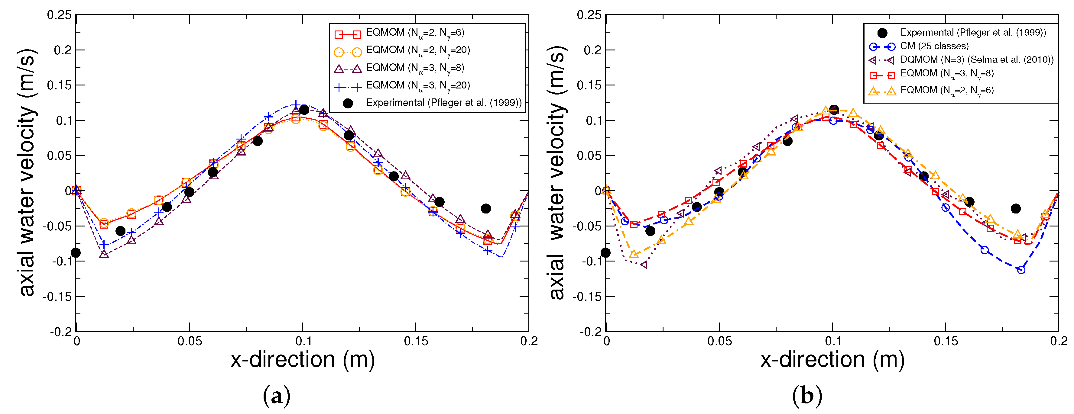
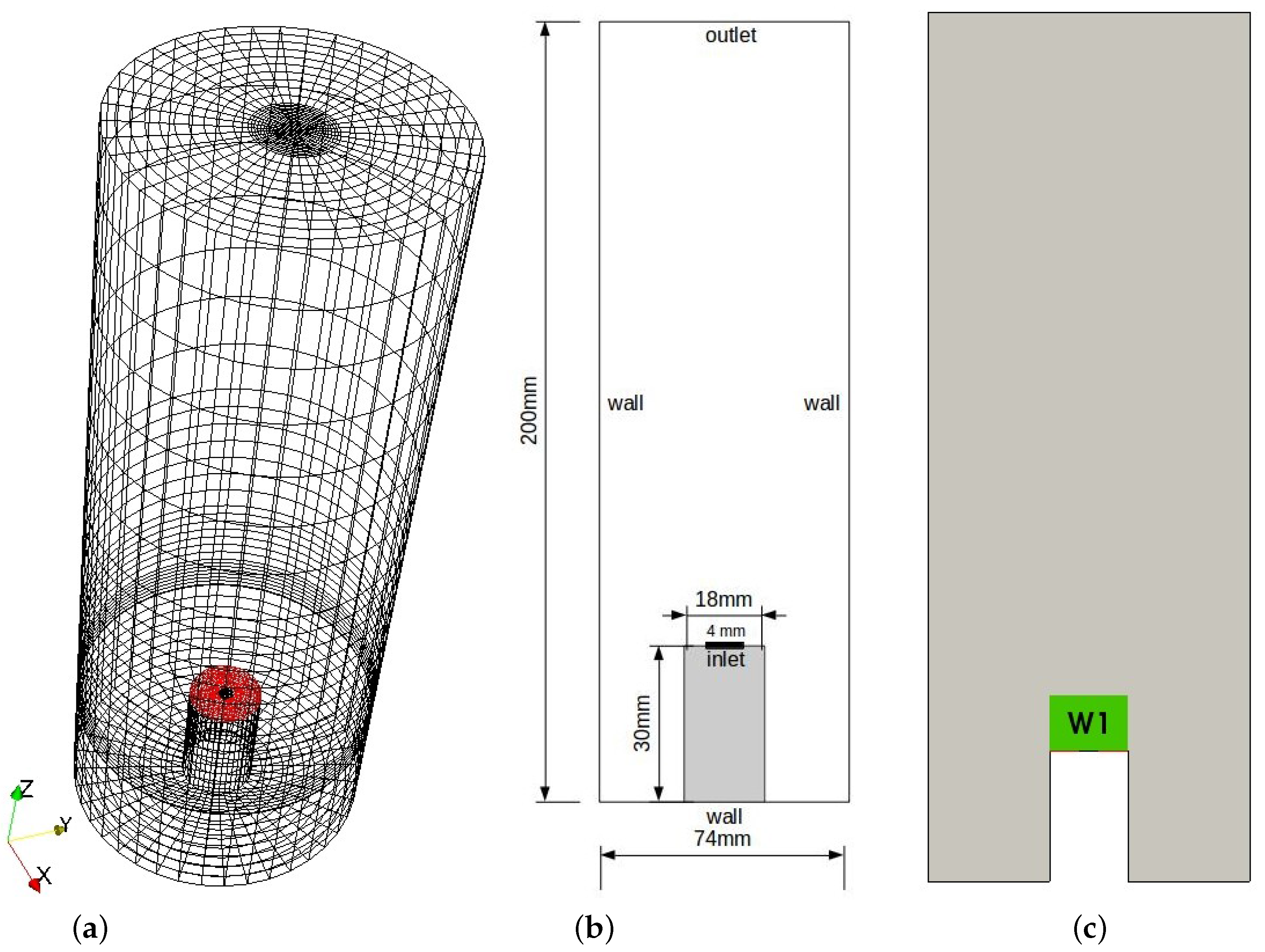
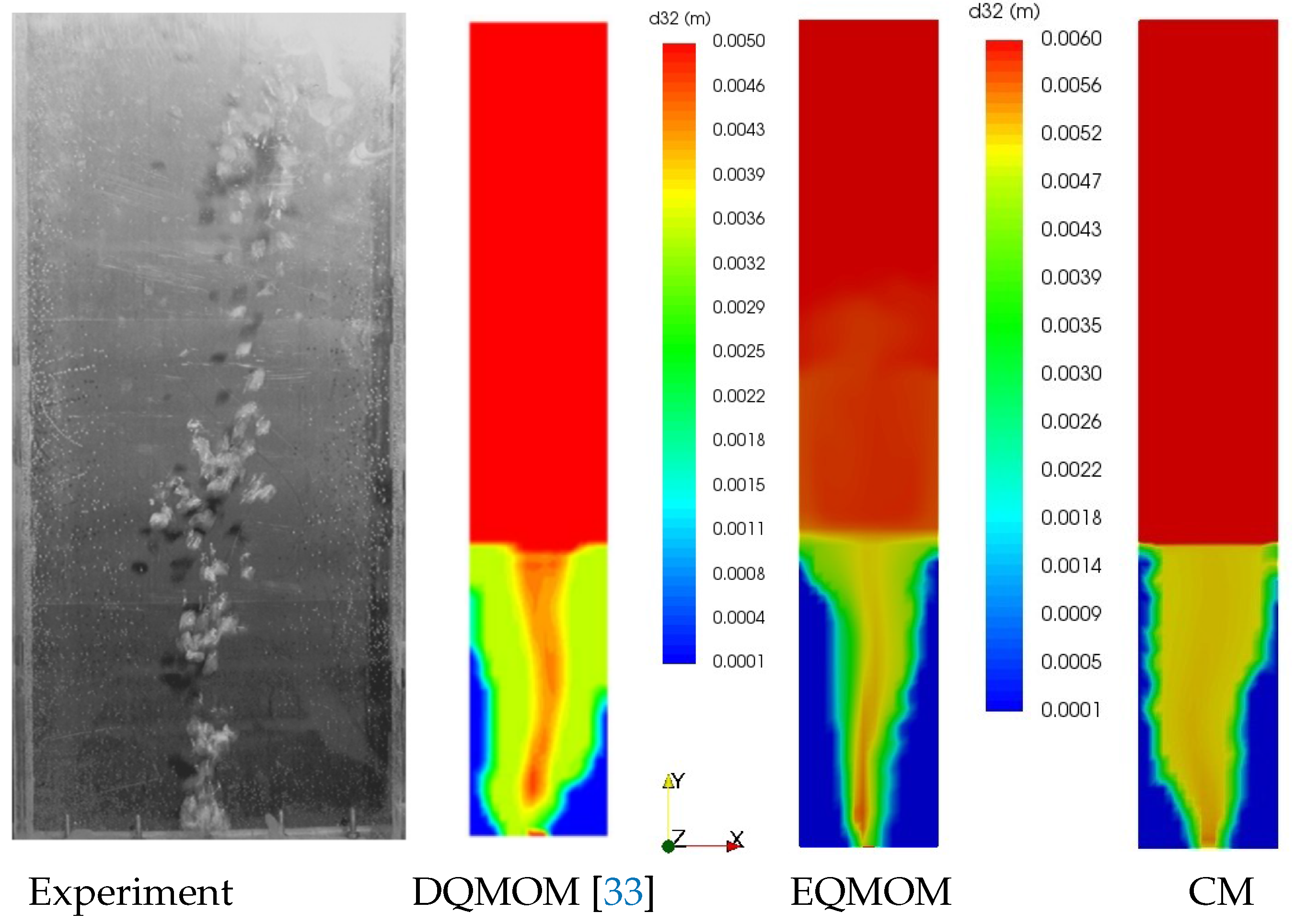
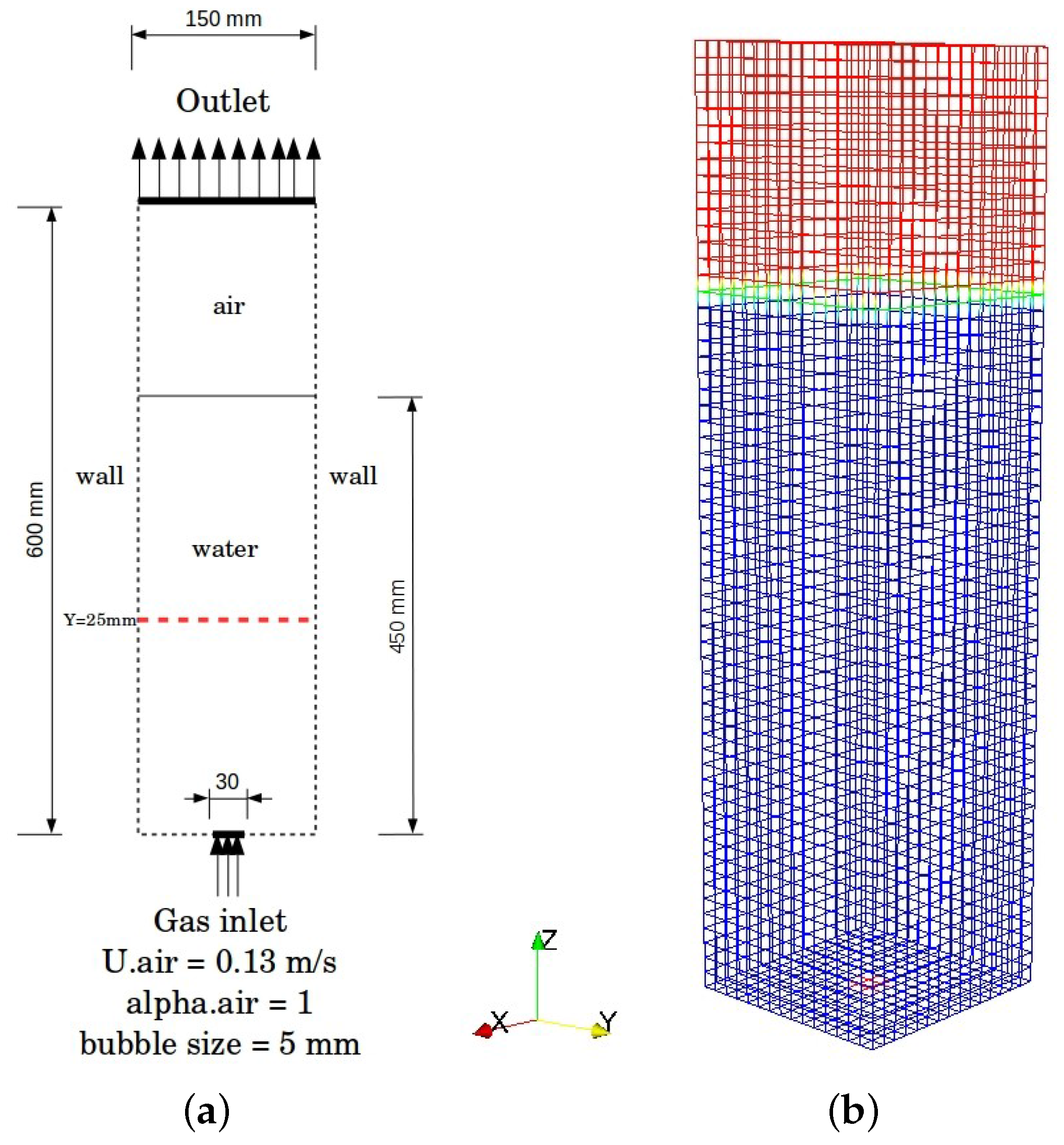
4.1. Test Case 1: Pseudo-2D Bubble Column

The first test case for the coupled Population Balance Model and Two Fluid Model (PBM-TFM) approach is a simple geometry (a rectangular bubble column [1]). The same test case was used in [33] to compare CM and DQMOM. Consequently, only the simulations with EQMOM were necessary to allow the comparison.
The dimensions and boundary conditions used to perform the simulations are shown in Figure 1, while Table 9 summarizes the models used in the simulations for this test case. Table 10, Table 11 and Table 12 demonstrates the boundary and initial conditions applied in CM, QMOM, EQMOM and DQMOM, respectively.
Figure 2 depicts a comparison between experimental measurements [62] and axial liquid velocity provided by the CFD-PBM solver on a line along y = 37 cm. The comparison confirms that the solver using EQMOM works properly for the bubble column. Figure 2a shows that the variation of secondary nodes does not have a significant impact. However, the increase of primary nodes from two to three provides better accuracy, as was expected. Figure 2b demonstrates the differences among population balance models. It is observed that EQMOM using three nodes represents a slight improvement in comparison with CM (25 classes) and DQMOM (three nodes). It is noteworthy that the CM (25 classes) computationally is very expensive [33]. By contrast, DQMOM and EQMOM have less computational demand.
Figure 3 demonstrates the radial bubble segregation based on the Sauter mean diameter contour. In fact, the bubble size decreases heading toward the wall due to breakage phenomena. However, the high gas phase fraction and coalescence events at the center of column lead to the creation of larger bubble sizes. As Figure 3 shows, Sauter mean diameter distributions predicted by the applied PBMs (DQMOM, EQMOM, CM) are qualitatively confirmed by comparison with experimental observation.
EQMOM is capable of providing a smooth reconstruction of the NDF for each arbitrary zone or cell in the computational domain. While this reconstruction is not unique for the set of transported moments, examining the reconstructed NDF can provide a better insight into the behavior of the dispersed phase. In order to plot NDF, weights and abscissae calculated by EQMOM and extracted from CFD-PBM solver are utilized to approximate Equation (37). Figure 4 indicates the shape of NDF in the liquid phase (water zone) at t = 60 s. It can be observed that the mean bubble diameter ranges from 1 mm to 6 mm, and thus, the monodispersity is not a suitable approximation. As can be observed from Figure 4a, the NDF is represented by a Dirac delta function for N = 2 , while Figure 4b exhibits a continuous NDF for N = 3 . This means the increase of the nodes in EQMOM configuration applied in the bubble column leads to the creation of a spread in bubble sizes, even locally.

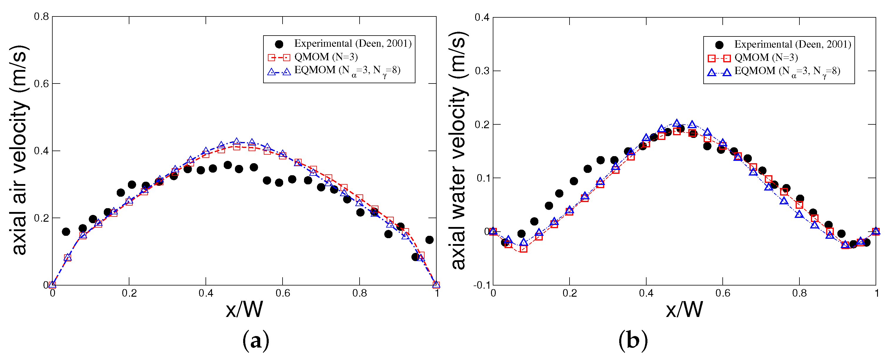
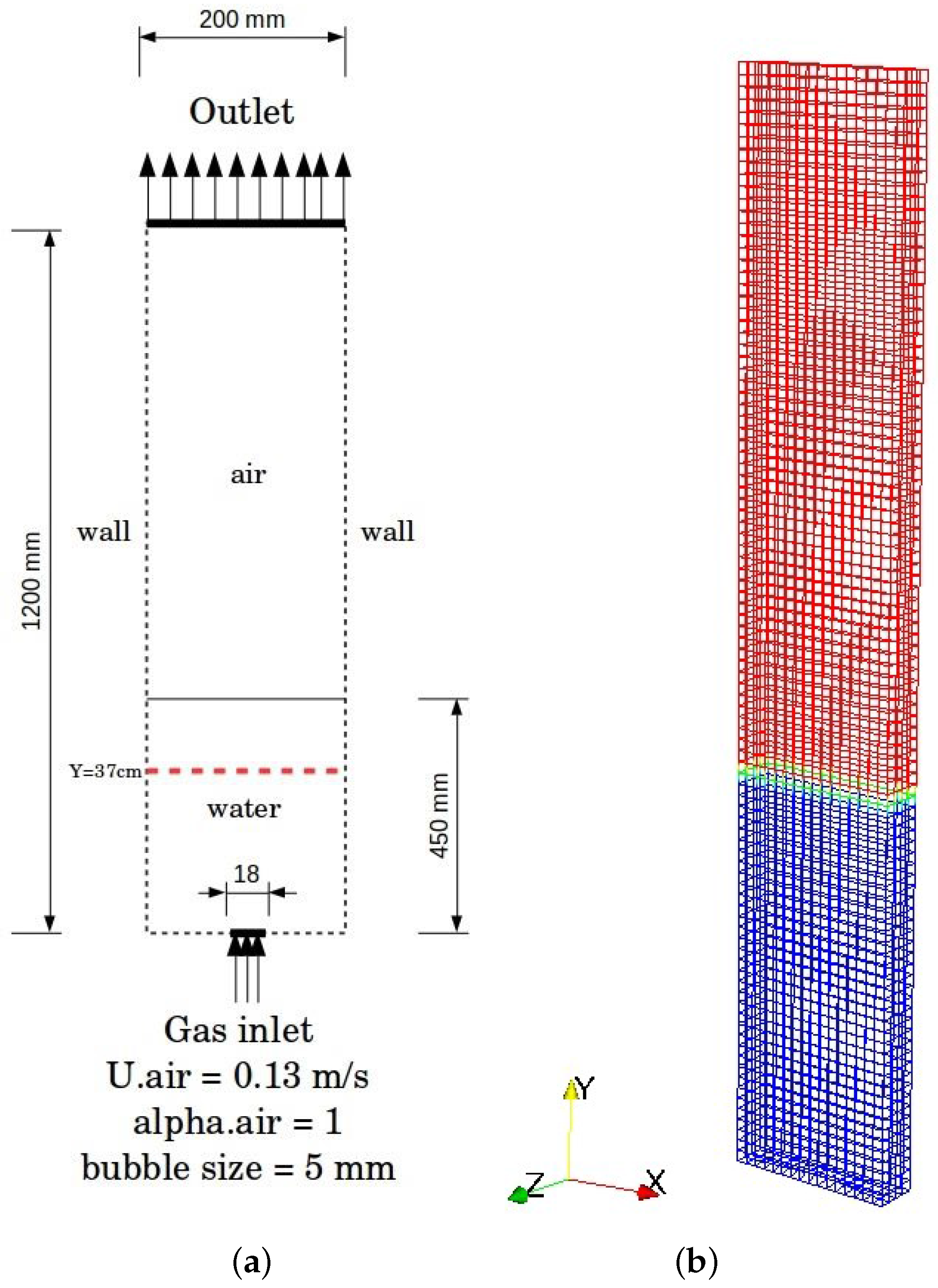
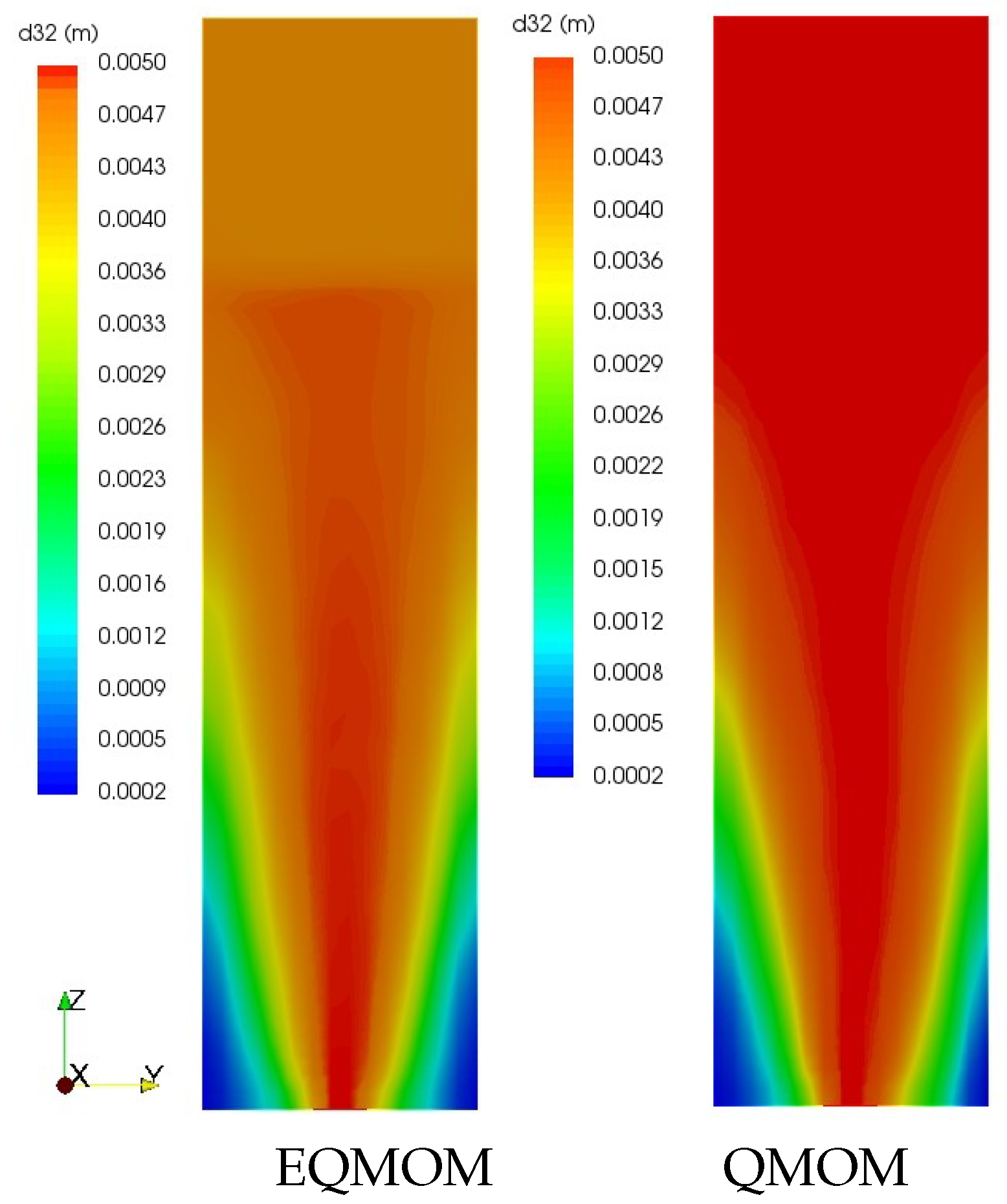
4.2. Test Case 2: 3D Bubble Column

For the second case, the coupled PBM-TFM solver was tested in a square bubble column (Deen [64]). The models used in the simulations are summarized in Table 13. This configuration is based on the work of Holzinger [10] in which the same test case was studied using a monodisperse bubble size distribution. In Test Case 2, QMOM and EQMOM simulations were performed.
The column has a square cross-section with W (width) = D (depth) = 0.15 m. The sparger is in the form of a square, the are of which is A i n = 0.03 × 0.03 m. The dimensions and boundary conditions are shown in Figure 5. The domain is discretized into 15 × 15 × 60 control volumes, a total of 13,500 cells. Figure 6 shows the comparison between QMOM and EQMOM with the experimental measurements reported by Deen [64]. Three nodes were used for QMOM, and three primary nodes were used for EQMOM. The EQMOM approach yielded a minor improvement in the gas velocity profile, while no change was observed through the liquid velocity profile. Likewise, the color maps of the Sauter mean diameter are similar for both methods, as shown in Figure 7. In spite of the similarity, the computational cost of EQMOM is higher than the QMOM method, as Madadi-Kandjani and Passalacqua [58] reported for a zero-dimension case, as well as the current simulation process.

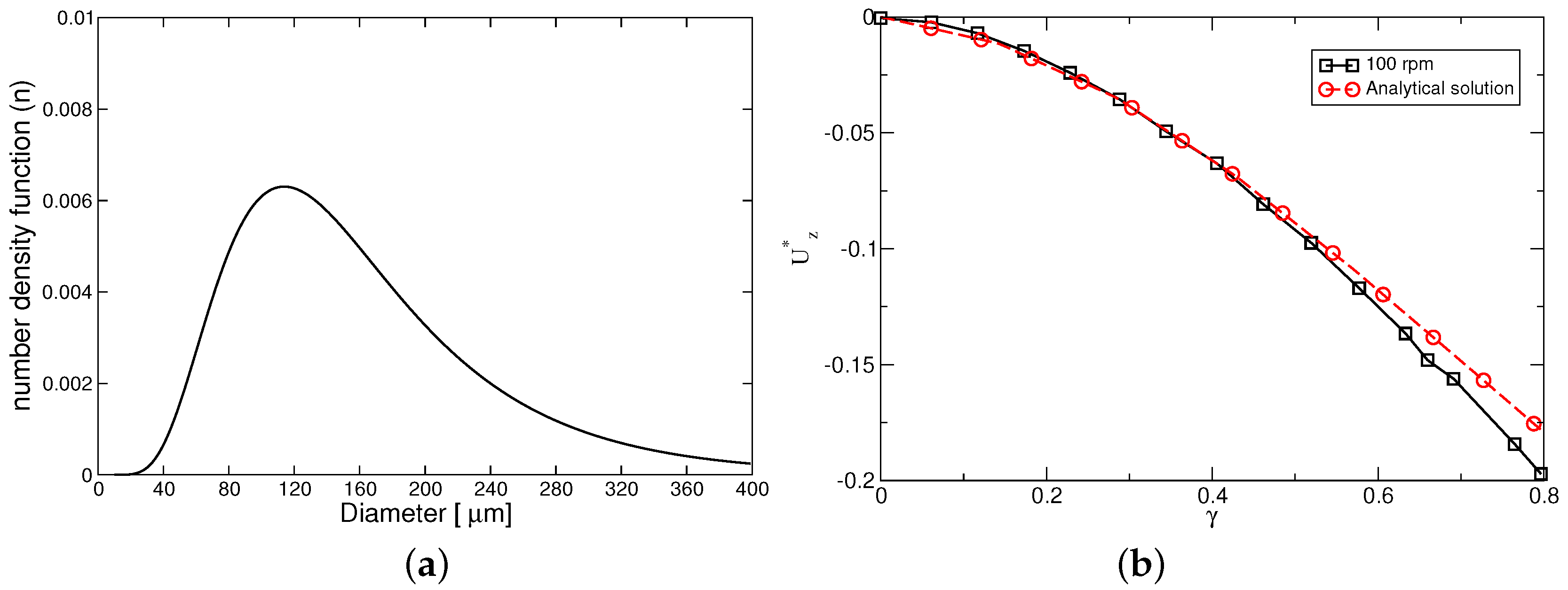
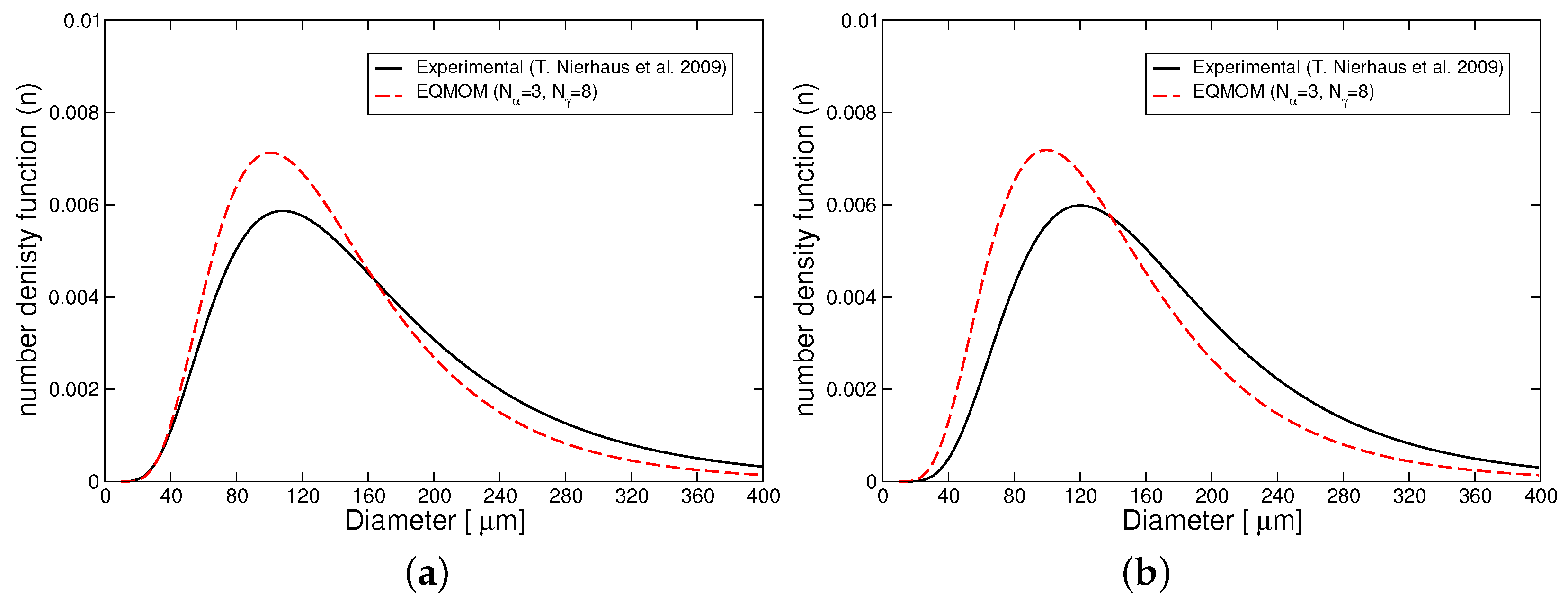
4.3. Test Case 3: Water Electrolysis Reactor

The bubbly flow in a water electrolysis reactor consisting of a gas evolution electrode was chosen as the third case. This decision is based on the simplicity of the case and on the availability of experimental data for the bubble size distribution. It was decided to investigate the Inverted Rotating Disk Electrode (IRDE) proposed by Van Parys et al. [65], which is composed of three electrodes as follows:
  • Reference electrode: Ag/AgCl saturated with KCl
  • Counter electrode: platinum grid
  • Working electrode (rotating electrode): made by embedding a platinum rod in an insulating Poly Vinylidene Fluoride (PVFD) cylinder.
When a potential difference is applied between electrodes, hydrogen is produced at the cathode and oxygen at the anode in the form of bubbles. In this case, we put aside the influence of the anode, because the experimental bubble distribution is only available over cathode and hydrogen bubbles. Consequently, the impact of oxygen bubbles is not taken into account in the simulation. The specifications of the IRDEreactor are presented in Figure 8. In this system, the rotating cathode is considered as an inlet boundary with imposed velocity, volume fraction and bubble size distribution. The angular component of the liquid velocity is set according to the rotational speed of working electrode ( ω = 100 and 250 rpm). According to the applied rotational speeds, the calculated Reynolds number is less than the critical ones [66]. Therefore, the flow regime is laminar, which allows neglecting source terms in the population balance model because of ϵ = 0 . In the present study, gas hold-up is extremely low. The bubbles follow the bulk flow and are affected by the continuous phase (water), but not vice versa. Hence, the flow field was calculated with a single-phase solver. The flow field obtained from the single-phase approach was then imported in the population balance solver, in order to advect the bubble size distribution imposed at the inlet and study how bubbles distribute in the IRDE. The settings, boundary and initial conditions used in the simulation are summarized in Table 14 and Table 15.
A distribution of bubble sizes is observed at the electrodes of the IRDE reactor. For this reason, the continuous distribution function reported by Nierhaus et al. [66] was used in the simulation and imposed at the electrode surface, which is treated as an inlet boundary for the gas phase (Figure 9a).
A grid with 34,300 hexahedra yielded sufficiently accurate results for the proposed problem and was selected for the IRDE study.
Nierhaus et al. [66] reported the experimental bubble size distributions in an optical window (W1) for two different rotating velocities, 100 rpm and 250 rpm. Figure 8 illustrates how the W 1 volume has been configured in the IRDE reactor. W1 was located above the electrode to enable tracking bubbles in the rising plume.
Figure 9b compares the computed axial velocity component profile u z * ( = u z ω z ν ) as a function of the dimensionless height ( γ = z δ ), where δ is the displacement thickness of the fluid boundary layer ( δ = ν ω z ). The comparison shows that the numerical results match with the analytical solution [68] in the region close to the electrode. The confirmed flow field applied in population balance calculations for its NDF consists of the accumulation and convection term (physical space).
To validate the CFD-PBM solver in IRDE, an analysis is applied to investigate the bubble size distribution in volume W1. The comparison of the bubble size distribution between the experimental study and current CFD-PBM using EQMOM (three nodes) is presented in Figure 10. The results thus obtained are compatible with experimental measurements (Figure 10a,b). The fair agreement confirms the assumptions in the PBM model, particularly for 150 rpm. In fact, since the bubble size is so small (low Stokes number), most of the effect is due to advection, and no segregation occurs.
In the case of 150 rpm, simulation data better match experimental data, while there is a disagreement for a higher rotational speed. The prime cause of the discrepancy might be the result of the neglect of size change effects in the PBM model.

5. Conclusions

In this paper, an analysis was performed for comparison among local Population Balance Models (PBM), CM, QMOM, DQMOM and EQMOM, based on three cases in the presence of bubbly flow. The purpose of the paper is to validate the CFD-PBM solver, which was applied for two different bubble columns and a water electrolysis reactor to predict the bubble size distribution. The originality of the OpenFOAM solver lies on the fact that it employs the novel method of PBM, which can accept the continuous bubble size distribution as a boundary condition. Moreover, the solver is able to export the distribution function for a specified region in an arbitrary time based on the EQMOM method. It was observed that the CFD-PBM using EQMOM provides a reasonable prediction, as well as CM consisting of 25 classes, but requires less computational demand compared with CM (Table 16). From the research that has been carried out, it is possible to conclude that QMOM and EQMOM have similar predictions. EQMOM is computationally more expensive than QMOM, although it is able to obtain a continuous NDF of the model. In order to simulate bubbly flow in the bubble column, it is proposed to use at least three nodes in the EQMOM technique. This minimum value is required to acquire a continuous NDF function. It is evident that the experimental and numerical NDF can be compared in the water electrolysis reactor (IRDE). Agreement is achieved using EQMOM in the IRDE reactor. The results proved that the most dominant term is advection in the PBM model.

Acknowledgments

The authors would like to thank Hydro-Québec and NSERC, which financially supported this study. A. P. would like to gratefully acknowledge the support of the U.S. National Science Foundation (NSF) under the Software Infrastructure for Sustained Innovation (SI 2 )–Scientific Software Elements (SSE) award NSF–ACI (Advanced Cyber Infrastructure) 1440443, which funded the development of the OpenQBMM framework.

Author Contributions

Ehsan Askari developed the libraries including CM, QMOM, Coalescence and Breakage kernels, carried out the simulations, performed the analysis and wrote the initial manuscript. Pierre Proulx supervised the project. Alberto Passalacqua is one of the team members of OpenQBMM. All authors discussed the results and contributed to the final manuscript.

Conflicts of Interest

The authors declare no conflict of interest.

Nomenclature

Symbols
a ( ζ ) breakage kernels 1
Bbirthm 3 s 1
b ( ν ) break-up frequency functions 1
C D drag coefficient
C l lift coefficient
C ν m virtual mass coefficient
c f increase coefficient of surface area
Ddeathm 3 s 1
dbubble diameterm
d 32 Sauter mean diameterm
E o Eotvos number
ffriction coefficient for flow around bubbles
f i volume fraction of bubble class i
F volumetric forceN m 3
g acceleration vector due to gravitym s 2
I = unit tensor
kturbulent kinetic energyj kg 1
Lbubble sizem
m ( ν ) mean number of daughter produced by breakage
nnumber density of bubblesm 3
Nangular velocityrad s 1
ppressurePa
P c coalescence efficiency or collision probability
p ( ν , ν ) pressureN m 2
r position vectorm
R interphase forceN m 3
R e Reynolds number
R ¯ ϕ e f f Reynolds (turbulent) and viscous stressm s 2
tTimes
U average velocity of phasem s 1
u i j bubble approaching turbulent velocitym s 1
W e Weber number
Greek Symbols
α Volume fraction
β constant 2.05 or s 1
β ( ζ , ζ ) coalescence rates 1
ϵ Turbulent kinetic energy dissipation ratem 2 s 3
θ i , j collision frequencym 3 s 1
μ dynamic viscosity of the continuous phaseN/m 3
λ eddy sizem
ρ densitykg/m 3
σ surface tension or varianceNm 1 or m
ζ internal variable
Ω B breakage frequencys 1
ν bubble size or kinematic viscositym 3 or m 2 / s
ξ i j size ratio d i / d j
Γ ( a , x ) incomplete Gamma function
η diameter ratio d i / d j
τ = stress tensorkg m 1 s 2
Subscripts
a g aggregation
b r breakage
e f f effective
Ggas phase
Lliquid phase
mmixture
iphase number
l a m laminar
tturbulent

References

  1. Bannari, R.; Kerdouss, F.; Selma, B.; Bannari, A.; Proulx, P. Three dimensional mathematical modeling of dispersed two-phase flow using class method of population balance in bubble columns. Comput. Chem. Eng. 2008, 32, 3224–3237. [Google Scholar] [CrossRef]
  2. Rusche, H. Computational Fluid Dynamics of Dispersed Two-Phase Flows at High Phase Fractions. Ph.D. Thesis, University of London, London, UK, 2002. [Google Scholar]
  3. Nierhaus, T. Modeling and Simulation of Dispersed Two-Phase Flow Transport Phenomena in Electrochemical Processes. Ph.D. Thesis, Universiteit Brussel, Brussels, Belgium, 2009. [Google Scholar]
  4. Karimi, M.; Droghetti, H.; Marchisio, D. PUFoam: A novel open-source CFD solver for the simulation of polyurethane foams. Comput. Phys. Commun. 2017, 217, 138–148. [Google Scholar] [CrossRef]
  5. Sequira, C.A.C.; Santos, D.M.F.; Sljukie, B.; Amaral, L. Physics of electrolytic gas evolution. Braz. J. Phys. 2013, 43, 199–208. [Google Scholar] [CrossRef]
  6. Leahy, M.J.; Phillip Schwarz, M. Modeling Natural Convection in Copper Electrorefining: Describing Turbulence Behavior for Industrial-Sized Systems. Metall. Mater. Trans. B 2011, 42, 875–890. [Google Scholar] [CrossRef]
  7. Leahy, M.J.; Philip Schwarz, M. Experimental Validation of a Computational Fluid Dynamics Model of Copper Electrowinning. Metall. Mater. Trans. B 2010, 41, 1247–1260. [Google Scholar] [CrossRef]
  8. Leahy, M.J.; Philip Schwarz, M. Computational Fluid Dynamics Modelling of Natural Convection in Copper Electrorefining. In Proceedings of the 16th Australasian Fluid Mechanics Conference, Gold Coast, Australia, 2–7 December 2007; pp. 112–116. [Google Scholar]
  9. Deen, N.G.; Solberg, T.; Hjertager, B.H. Flow generated by an aerated Rushton impeller: Two-phase PIV Experiments and numerical simulations. Can. J. Chem. Eng. 2002, 80, 1–15. [Google Scholar] [CrossRef]
  10. Holzinger, G. Eulerian Two-Phase Simulation of the Floating Process with OpenFOAM. Ph.D. Thesis, Johannes Kepler Universitat Linz, Linz, Austria, 2016. [Google Scholar]
  11. Friberg, P.C. Three-Dimensional Modeling and Simulations of Gas-Liquid Flows Processes in Bioreactors. Ph.D. Thesis, Telemark Institute of Technology, Bø, Norway, 1998. [Google Scholar]
  12. Morud, K.E.; Hjertager, B.H. LDA measurements and CFD modeling of gas-liquid flow in a stirred vessel. Chem. Eng. Sci. 1996, 51, 233–249. [Google Scholar] [CrossRef]
  13. Ranade, V.V.; Deshpande, V.R. Gas-liquid flow in stirred vessels: Trailing vortices and gas accumulation behind impeller blades. Chem. Eng. Sci. 1999, 54, 2305–2315. [Google Scholar] [CrossRef]
  14. Ranade, V.V. An efficient computational model for simulating flow in stirred vessels: A case of Rushton Turbine. Chem. Eng. Sci. 1997, 52, 4473–4484. [Google Scholar] [CrossRef]
  15. Schwarz, M.P.; Turner, W.J. Applicability of the standard k-e turbulence model to gas-stirred baths. Appl. Math. Model. 1988, 12, 273–279. [Google Scholar] [CrossRef]
  16. Schwarz, M.P. Simulation of gas injection into liquid melts. Appl. Math. Model. 1996, 20, 41–51. [Google Scholar] [CrossRef]
  17. Kresta, S.M.; Etchells, A.W., III; Dickey, D.S.; Atiemo-Obeng, V.A. Advances In Industrial Mixing; John Wiley & Sons: New York, NY, USA, 2016. [Google Scholar]
  18. Kerdouss, F.; Bannari, A.; Proulx, P. CFD modeling of gas dispersion and bubble size in a double turbine stirred tank. Chem. Eng. Sci. 2006, 61, 3313–3322. [Google Scholar] [CrossRef]
  19. Ishii, M.; Kim, S.; Uhle, J. Interfacial area transport equation: Model development and benchmark experiments. Int. J. Heat Mass Transf. 2002, 45, 3111–3123. [Google Scholar] [CrossRef]
  20. Dhanasekharan, K.; Sanyal, J.; Jain, A.; Haidari, A. A generalize approach to model oxygen transfer in boreactors using population balances and computational fluid dynamics. Chem. Eng. Sci. 2005, 60, 213–218. [Google Scholar] [CrossRef]
  21. Venneker, B.C.H.; Derksen, J.J.; Van den Akker, H.E.A. Population balance modeling of aerated stirred vessels based on CFD. AIChE J. 2002, 48, 673–684. [Google Scholar] [CrossRef]
  22. Balakin, B.V.; Hoffmann, A.C.; Kosinski, P. Coupling STAR-CD with a population balance technique based on the classes method. Powder Technol. 2014, 257, 47–54. [Google Scholar] [CrossRef]
  23. Becker, P.J.; Puel, F.; Henry, R.; Sheibat-Othman, N. Investigation of discrete population balance models and breakage kernels for dilute emulsification systems. Ind. Eng. Chem. Res. 2011, 50, 11358–11374. [Google Scholar] [CrossRef]
  24. Kumar, S.; Ramkrishna, D. On the solution of population balance equations by discretization-I. A fixed pivot technique. Chem. Eng. Sci. 1996, 51, 1311–1332. [Google Scholar] [CrossRef]
  25. Kumar, S.; Ramkrishna, D. On the solution of population balance equations by discretization-II. A moving pivot technique. Chem. Eng. Sci. 1996, 51, 1333–1342. [Google Scholar] [CrossRef]
  26. Puel, F.; Fvotte, G.; Klein, J.P. Simulation and analysis of industrial crystal-lization processes through multidimensional population balance equations. Chem. Eng. Sci. 2003, 58, 3715–3727. [Google Scholar] [CrossRef]
  27. McGraw, R. Description ofaerosol dynamics by the quadrature method ofmoments. Aerosol Sci. Technol. 1997, 27, 255–265. [Google Scholar] [CrossRef]
  28. Marchisio, D.L.; Vigil, R.D.; Fox, R.O. Quadrature method of moments for aggregation-breakage processes. J. Colloid Interface Sci. 2003, 258, 322–334. [Google Scholar] [CrossRef]
  29. Marchisio, D.L.; Pikturna, J.T.; Fox, R.O.; Vigil, R.D. Quadrature method of moments for population-balance equations. AIChE J. 2003, 49, 1266–1276. [Google Scholar] [CrossRef]
  30. Marchisio, D.L.; Vigil, R.D.; Fox, R.O. Implementation of the quadrature method of moments in CFD codes for aggregation-breakage problems. Chem. Eng. Sci. 2003, 139, 3337–3351. [Google Scholar] [CrossRef]
  31. Sanyal, J.; Marchisio, D.L.; Fox, R.O.; Dhanasekharan, K. On the comparaison between population balance models for CFD simulation of bubble columns. Ind. Eng. Chem. Res. 2005, 44, 5063–5072. [Google Scholar] [CrossRef]
  32. Silva, L.; Lage, P. Development and implementation of a polydispersed multiphase model in OpenFOAM. Comput. Chem. Eng. 2011, 35, 2653–2666. [Google Scholar] [CrossRef]
  33. Selma, B.; Bannari, R.; Proulx, P. Simulation of bubbly flows: Comparison between direct quadrature method of moments (DQMOM) and method of classes. Chem. Eng. Sci. 2010, 65, 1925–9141. [Google Scholar] [CrossRef]
  34. Marchisio, D.L.; Fox, R.O. Solution of population balance equations using the direct quadrature method of moments. J. Aerosol Sci. 2005, 36, 43–73. [Google Scholar] [CrossRef]
  35. Fox, R.; Laurant, F.; Massot, M. Numerical simulation of spray coalescence in an Eulerian framework: Direct quadrature method of moments and multi-fluid method. J. Comput. Phys. 2008, 227, 3058–3088. [Google Scholar] [CrossRef]
  36. Yuan, C.; Laurant, F.; Fox, R.O. An extended quadrature method of moments for population balance equations. J. Aerosol Sci. 2012, 32, 1111–1116. [Google Scholar] [CrossRef]
  37. Li, D.; Gao, Z.; Buffo, A.; Podgorska, W.; Marchisio, D.L. Droplet breakage and coalescence in liquid-liquid dispersions: Comparison of different kernels with EQMOM and QMOM. AIChE J. 2017, 63, 2293–2311. [Google Scholar] [CrossRef]
  38. Gimbun, J.; Rielly, C.D.; Nagy, Z.K. Modelling of mass transfer in gas-liquid stirred tanks agitated by Rushton turbin and CD-6 impeller: A scale up study. Chem. Eng. Res. Des. 2017, 87, 437–451. [Google Scholar] [CrossRef] [Green Version]
  39. Gupta, A.; Roy, S. Euler–Euler simulation of bubbly flow in a rectangular bubble column: Experimental validation with Radioactive Particle Tracking. Chem. Eng. J. 2013, 225, 818–836. [Google Scholar] [CrossRef]
  40. Askari, E.; Lemieux, G.S.P.; Vieira, C.B.; Litrico, G.; Proulx, P. Simulation of Bubbly Flow and Mass Transfer in a Turbulent Gas-Liquid Stirred Tank with CFD-PBM solver in OpenFOAM: EQMOM applicationg. In Proceedings of the 15th International Conference of Numerical Analysis and Applied Mathematics, Thessaloniki, Greece, 25–30 September 2017. [Google Scholar]
  41. OpenQBMM. An open-source implementation of Quadrature-Based Moment Methods. Zenodo 2017. [Google Scholar] [CrossRef]
  42. Schiller, L.; Naumann, Z. A drag coefficient correlation. Z. Ver. Deutsch. Ing. 1935, 77, 318–320. [Google Scholar]
  43. Ishii, M.; Zuber, N. Drag coefficient and relative velocity in bubbly, droplet or particulate flows. AIChE J. 1979, 25, 843–855. [Google Scholar] [CrossRef]
  44. Tomiyama, A.; Celata, G.; Hosokawa, S.; Yoshida, S. Terminal velocity of single bubbles in surface tension force dominant regime. Int. J. Multiph. Flow 2002, 28, 1497–1519. [Google Scholar] [CrossRef]
  45. Behzadi, B.; Issa, R.I.; Rusche, H. Modelling of dispersed bubble and droplet flow at high phase fractions. Chem. Eng. Sci. 2004, 59, 759–770. [Google Scholar] [CrossRef]
  46. Luo, H.; Svendsen, H.F. Theoretical model for drop and bubble breakup in turbulent dispersions. AIChE J. 1996, 42, 1225–1233. [Google Scholar] [CrossRef]
  47. Hagesather, L.; Jakobsen, H.A.; Hjarbo, K.; Svendsen, H.F. A coalescence and breakup module for implementation in CFD codes. Comput. Aided Chem. Eng. 2000, 8, 367–372. [Google Scholar]
  48. Saffman, P.G.; Turner, J.S. On the collision of drops in turbulent clouds. J. Fluid Mech. 1956, 1, 16–30. [Google Scholar] [CrossRef]
  49. Marchisio, D.L.; Fox, R.O. Multiphase Reacting Flows: Modelling and Simulation; Springer: NewYork, NU, USA, 2007. [Google Scholar]
  50. Ramkrishna, D. Population Balances; Academic Press: San Diego, CA, USA, 2000. [Google Scholar]
  51. Abraham, F. Homogeneous Nucleation Theory; Academic Press: New York, NY, USA, 1974. [Google Scholar]
  52. Tomasoni, F. Non-Intrusive Assessment of Transport Phenomena at Gas-Evolving Electrodes. Ph.D. Thesis, Vrije Universiteit Brussel, Brussels, Belgium, 2010. [Google Scholar]
  53. Lo, S. Application of Population Balance to CFD Modeling of Bubbly Flow via the MUSIG Model; AEA Technology: Harwell, UK, 1996; p. 1096. [Google Scholar]
  54. Yuan, C.; Kong, B.; Passalacqua, A.; Fox, R.O. An extended quadrature-based mass-velocity moment model for polydisperse bubbly flows. Can. J. Chem. Eng. 2014, 92, 2053–2066. [Google Scholar] [CrossRef]
  55. Fan, R.; Marchisio, D.L.; Fox, R.O. Application of the direct quadrature method of moments to polydisperse gas–solid fluidized beds. Powder Technol. 2004, 139, 7–20. [Google Scholar] [CrossRef]
  56. Bove, S. Computational Fluid Dynamics of Gas–Liquid Flows Including Bubble Population Balances. Ph.D. Thesis, Aalborg University, Aalborg, Denmark, 2005. [Google Scholar]
  57. Nguyen, T.T.; Laurent, F.; Fox, R.O.; Massot, M. Solution of population balance equations in applications with fine particles: Mathematical modeling and numerical schemes. J. Comput. Phys. 2016, 325, 129–156. [Google Scholar] [CrossRef]
  58. Madadi-Kandjani, E.; Passalacqua, A. An extended quadrature-based moment method with log-normal kernel density functions. Chem. Eng. Sci. 2015, 131, 323–339. [Google Scholar] [CrossRef]
  59. Kerdouss, F.; Bannari, A.; Proulx, P. Two-phase mass transfer coefficient prediction in stirred vessel with a CFD model. Comput. Chem. Eng. 2007, 32, 1943–1955. [Google Scholar] [CrossRef]
  60. Kerdouss, F.; Kiss, L.; Proulx, P.; Bilodeau, J.F.; Dupuis, C. Mixing Characteristics of an axial flow rotor: Experimental and numerical study. Int. J. Chem. React. Eng. 2005, 3. [Google Scholar] [CrossRef]
  61. OpenFOAM 4.0; The OpenFOAM Foundation: London, UK, 2017.
  62. Pfleger, D.; Gomes, S.; Gilbert, N.; Wagner, H.G. Hydrodynamic simulations of laboratory scale bubble columns. Fundamental studies of the Eulerian–Eulerian modeling approach. Chem. Eng. Sci. 1999, 54, 5091–5099. [Google Scholar] [CrossRef]
  63. Buwa, V.V.; Deo, D.S.; Ranade, V.V. Eulerian–Lagrangian simulations of unsteady gas–liquid flows in bubble columns. Int. J. Multiph. Flow 2006, 32, 864–885. [Google Scholar] [CrossRef]
  64. Deen, N.G. An Experimental and Computational Study of Fluid Dynamics in Gas-Liquid Chemical Reactors. Ph.D. Thesis, Aalborg University Esbjerg, Esbjerg, Denmark, 2001. [Google Scholar]
  65. Van Parys, H.; Tourwe, E.; Breugelmans, T.; Depauw, M.; Deconinck, J.; Hubin, A. Modeling of mass and charge transfer in an inverted rotating disk electrode (IRDE) reactor. J. Electroanal. Chem. 2009, 622, 44–50. [Google Scholar] [CrossRef]
  66. Nierhaus, T.; Parys, H.V.; Dehaeck, S.; Beeck, J.V.; Deconinck, H.; Deconinck, J.; Hubinc, A. Simulation of the Two-Phase Flow Hydrodynamics in an IRDE Reactor. J. Electrochem. Soc. 2009, 156, 139–148. [Google Scholar] [CrossRef]
  67. SuperMarine. Available online: https://github.com/Spationaute/SuperMarine (accessed on 8 January 2018).
  68. Cochran, W.G. The flow due to a rotating disc. Math. Proc. Camb. Philos. Soc. 1934, 30, 365–375. [Google Scholar] [CrossRef]
Figure 1. (a) Dimension and boundary conditions in the bubble column [1] and (b) mesh.
Chemengineering 02 00008 g001
Figure 2. Profile of axial liquid velocity through a line at y = 37 cm from the bottom of the bubble column. (a) The variation of primary and secondary nodes and their effects on the predicted velocity profile. (b) The comparison among CM (classes), DQMOM (3 nodes), EQMOM (3 nodes) and EQMOM (2 nodes).
Chemengineering 02 00008 g002
Figure 3. Experimental snapshot of a meandering bubble plume by Buwa et al. [63] and the predicted Sauter mean diameter using DQMOM ([33]), EQMOM and CM.
Chemengineering 02 00008 g003
Figure 4. Number density function in water zone (liquid phase) using EQMOM (a) N α = 2 and (b) N α = 3 .
Chemengineering 02 00008 g004
Figure 5. (a) Dimension and boundary condition in the bubble column (Deen [64]) and (b) the mesh (13,500 cells) in the case of Deen [64].
Chemengineering 02 00008 g005
Figure 6. Comparison between EQMOM and QMOM against experimental data: (a) axial gas velocity and (b) axial liquid velocity for the case of Deen [64].
Chemengineering 02 00008 g006
Figure 7. Color maps of time-averaged Sauter diameter along the plane located in the middle of the column of Deen [64].
Chemengineering 02 00008 g007
Figure 8. (a) Schematic of hexahedral mesh [67]. (b) The specifications of the reactor and (c) the location of volume W1.
Chemengineering 02 00008 g008
Figure 9. (a) The continuous distribution function imposed at the electrode surface (Nierhaus et al. [66]); (b) mean axial velocity component profile u z * = u z ω z ν and comparison to the analytical solution.
Chemengineering 02 00008 g009
Figure 10. Bubble size distribution in W1 for (a) EQMOM (three nodes) and rpm = 100; (b) EQMOM (three nodes) and rpm = 250.
Chemengineering 02 00008 g010
Table 1. The most remarkable studies in the field of bubbly flow modeling using Population Balance Model (PBM). CM, Method of Classes; EQMOM, Extended Quadrature Method of Moments; DQMOM, Direct Quadrature Method of Moments.
ReferenceTest CasePBMHypothesesRemarks
Bannari et al. [1]bubble columnCMaccumulation, advection, coalescence, breakageConstant mean bubble size does not give satisfactory results compared to those based on PBM; 25 classes give better results
Gimbun et al. [38]gas-liquid stirred tankQMOMaccumulation, coalescence, breakageBetter agreement is achieved using PBM compared to a uniform bubble size
Li et al. [37]liquid-liquid stirred tankEQMOM and QMOMaccumulation, advection, coalescence, breakageSimilar predictions for EQMOM and QMOM; EQMOM provides a continuous BSD
Selma et al. [33]gas-liquid stirred tank; bubble columnDQMOM and CMaccumulation, advection, coalescence, breakageHigh number of classes is required; CM is computationally heavy; DQMOM is much more efficient (computationally) compared to CM
Gupta and Roy [39]bubble columnDQMOM and QMOMaccumulation, coalescence, breakageA summary of studies done on bubble columns flow modeling using PBM; no significant difference between DQMOM and QMOM
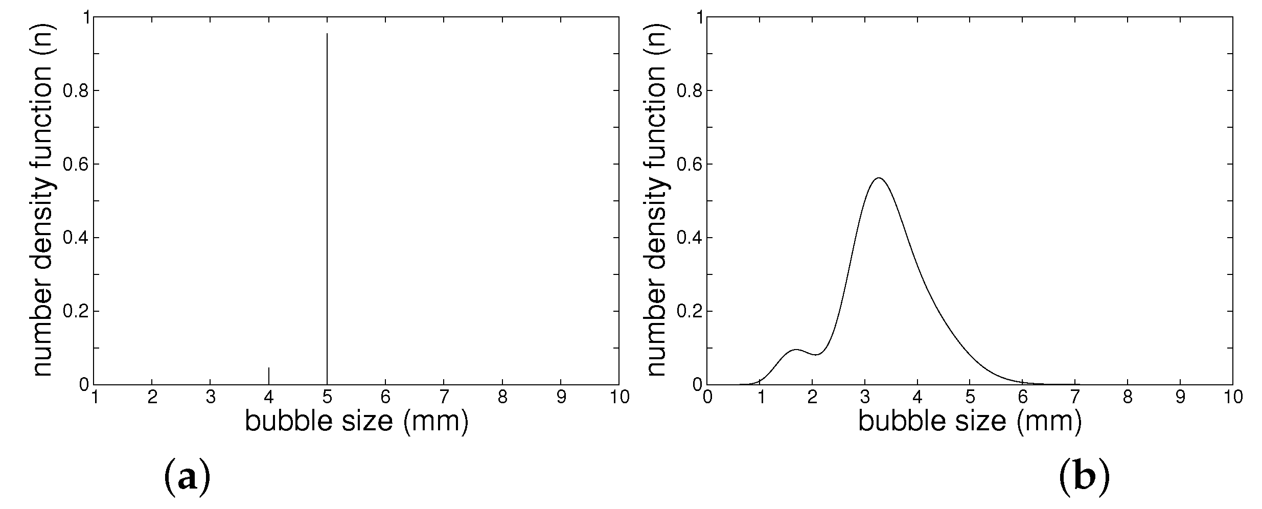
Askari et al. [40]gas-liquid stirred tankEQMOMaccumulation, coalescence, breakageThe agreement between experimental data and simulation results using EQMOM; reconstruction of bubble size distribution
Table 2. An overview of locally polydisperse PBMs. NDF, Number Density Function.
PBMAdvantagesDisadvantages
CMIntuitive and accurateComputationally intensive
QMOMWide range of bubble sizes with a reduced computational costDisabled in case of null internal coordinates
DQMOMWide range of bubble sizes with a reduced computational costShortcomings related to non-conservative quantities (weights and abscissas)
EQMOMWide range of bubble sizes with a reduced computational cost (ONLYcompared to CM) and reconstruction capability of continuous NDFHeavy computation compared to QMOM and DQMOM
Table 3. Governing equations of the CFD-PBM model.
EquationFormulation
Continuity (single-phase) ρ t + · ρ U = 0
Momentum (single-phase) t ρ U + · ( ρ U U ) = p + · τ ¯ ¯ effi
Continuity (multi-phase) t ρ i α i + · α i ρ i U i = 0.0
Reynolds stress tensor τ ¯ ¯ effi = μ lam + μ t U + U T 2 3 ρ k + μ lam + μ t · U I ¯ ¯
Momentum (multi-phase) t ρ i α i U i + · α i ρ i U i U i = α i p + · ( α i τ ¯ ¯ effi , i ) + R i + F i + α i ρ i g
Interfacial momentum exchange R G = R L = R G , drag + R G , lift + R G , vm
Liquid-gas exchange coefficient K = 3 4 ρ L α G C D d 32 U G U L ( U G U L ) + α G C l ρ L U r × ( × U L ) + α L C vm ρ L D L U L D t D G U G D t
Schiller–Naumann drag coefficient [42] C D = 24 Re 1 + 0.15 Re 0.687 Re 1000 0.44 otherwise
Ishii–Zuber drag coefficient [43] C D = max { min [ 2 3 Eo , 8 3 ] , 24 Re ( 1 + 0.1 Re 0.75 ) }
Tomiyama lift coefficient [44] C l = min ( 0.288 tanh ( 0.121 Re ) , f ( Eo G ) ) Eo G < 4 f ( Eo G ) 4 Eo G 10.7
Mixture k- ϵ model [45] t ρ m k m + · ρ m U m k m = · μ t , m σ k k m + P k m ρ m ϵ m + S k m
t ρ m ϵ m + · ρ m U m ϵ m = · μ t , m σ ϵ k m + ϵ m k m C 1 ϵ G k , m C 2 ϵ ρ m ϵ m + C ϵ 3 ϵ m ϵ k S k m
Break-up rate function [46] Ω B ( d j : d i ) = 3 k 1 ( 1 α ) 11 b 8 / 11 n j ϵ d j 2 1 / 3 { Γ ( 8 / 11 , t m ) Γ ( 8 / 11 , b ) + 2 b 3 / 11 ( Γ ( 5 / 11 , t m ) Γ ( 5 / 11 , b ) )
+ b 6 / 11 ( Γ ( 2 / 11 , t m ) Γ ( 2 / 11 , b ) ) }
Coalescence rate [47] β ( d i , d j ) = θ i j P c
Coalescence frequency [48] θ ( i , j ) = π 4 n i n j ( d i + d j ) 2 ϵ 1 / 3 d i 2 / 3 + d j 2 / 3 1 / 2
Coalescence efficiency [47] P C ( d i , d j ) = exp c 0.75 ( 1 + ξ i j 2 ) ( 1 + ξ i j 3 ) 1 / 2 ( ρ d / ρ c + 0.5 ) 1 / 2 ( 1 + ξ i j ) 3 We i j 1 / 2
Table 4. Values of r and s used in different classes.
Number of Classes7111525
Value of r35712
Value of s21.51571.34591.1892
Table 5. Values of weights used in Gaussian quadrature.
W 1 W 2 W 3 W 4 W 5
35 + 2 70 63 35 2 70 63 0 35 2 70 63 35 + 2 70 63
Table 6. Boundary and initial condition for f i equations.
Boundary ConditionsInitial Condition
InletWallOutletInlet value
f i = 1 i = 2 r 0 i 2 r NeumannNeumann
Table 7. Boundary conditions, initial conditions and divergence scheme corresponding m i equations.
Boundary ConditionsInitial Condition
InletWallOutletInlet value
Equation (32)NeumannNeumann
Table 8. Boundary conditions and initial condition for DQMOM equations.
Boundary ConditionsInitial Condition
InletWallOutletInlet value
L i and W i corresponding to m i NeumannNeumann
Table 9. Models used in the simulation of the bubble column of Pfleger et al. [62]. TFM, Two-Fluid Model.
SettingsModel
Two-phase flowTwo-fluid model (TFM)
DragSchiller and Naumann [42]
LiftTomiyama et al. [44]
Virtual mass C v m = 0.25 [33]
TurbulenceStandard k- ϵ model
Population balanceCM and EQMOM
CoalescenceHagesather et al. [47]
BreakageLuo and Svendsen [46]
Table 10. Boundary and initial conditions for f i equations (25 classes).
Boundary ConditionsInitial Condition
InletWallOutletInlet value
f i = 1 i = 12 0 i 12 NeumannNeumann
Table 11. Boundary and initial conditions for m i equations used in the QMOM and EQMOM methods (Test Cases I and II).
Boundary ConditionsInitial Condition
InletWallOutletInlet value
m i = 1 i = 0 5 i = 1 25 i = 2 125 i = 3 625 i = 4 3125 i = 5 15,625 i = 5 NeumannNeumann
Table 12. Boundary and initial conditions for W i and L i equations used in the DQMOM method [33].
Boundary ConditionsInitial Condition
InletWallOutlet W i = 0.33 i = 0 0.33 i = 1 0.34 i = 2 L i = 0.001 i = 0 0.002 i = 1 0.003 i = 2
W i = 0.1667 i = 0 0.6667 i = 1 0.1667 i = 2 L i = 3.26 i = 0 5.00 i = 1 6.73 i = 2 NeumannNeumann
Table 13. Overview of the models used in the solver.
SettingsModel
Two-phase flowTwo-fluid model
DragIshii and Zuber [43]
Lift C l = 0.5
Virtual mass C v m = 0.5
TurbulenceBehzadi et al. [45]
Population balanceEQMOM and QMOM
CoalescenceHagesather et al. [47]
BreakageLuo and Svendsen [46]
Table 14. Models used in the simulations of Test Case 3.
SettingsModel
single-phase flow-
laminar-
population balanceEQMOM
coalescenceno
breakageno
Table 15. Boundary and initial condition for m i equations used in Test Case 3.
Boundary ConditionsInitial Condition
InletWallOutletInlet value
m i = 1 i = 0 145 i = 1 26,801 i = 2 6.31 × 10 6 i = 3 1.89 × 10 9 i = 4 7.26 × 10 11 i = 5 3.54 × 10 14 i = 6 NeumannNeumann
Table 16. Normalized computational costs of applied PBMs in Test Cases 1 and 2.
CaseDQMOM [33]CM (25 Classes)QMOM (n = 3)EQMOM (n = 2)EQMOM (n = 3)
Test Case 115-1.31.4
Test Case 2--1-1.5

