Evaluation of Maintenance and EOL Operation Performance of Sensor-Embedded Laptops


Department of Mechanical and Industrial Engineering, Northeastern University, Boston, MA 02115, USA
*
Author to whom correspondence should be addressed.
Logistics 2018, 2(1), 3; https://doi.org/10.3390/logistics2010003
Submission received: 20 November 2017
/
Revised: 2 January 2018
/
Accepted: 2 January 2018
/
Published: 8 January 2018
(This article belongs to the Section Artificial Intelligence, Logistics Analytics, and Automation)
Abstract
:Sensors are commonly employed to monitor products during their life cycles and to remotely and continuously track their usage patterns. Installing sensors into products can help generate useful data related to the conditions of products and their components, and this information can subsequently be used to inform EOL decision-making. As such, embedded sensors can enhance the performance of EOL product processing operations. The information collected by the sensors can also be used to estimate and predict product failures, thereby helping to improve maintenance operations. This paper describes a study in which system maintenance and EOL processes were combined and closed-loop supply chain systems were constructed to analyze the financial contribution that sensors can make to these procedures by using discrete event simulation to model and compare regular systems and sensor-embedded systems. The factors that had an impact on the performance measures, such as disassembly cost, maintenance cost, inspection cost, sales revenues, and profitability, were determined and a design of experiments study was carried out. The experiment results were compared, and pairwise t-tests were executed. The results reveal that sensor-embedded systems are significantly superior to regular systems in terms of the identified performance measures.
1. Introduction
Constructing and sustaining efficient closed-loop supply chain systems has become extremely important for organizations because technology advances very quickly and the manufacturing business is highly competitive. In addition, consumers’ increasing environmental awareness and the introduction of legislation that governs the management of EOL products has forced firms to increase the amount of EOL products that are recovered and reprocessed as part of a closed-loop supply chain. While these activities come at a cost, they are also a source of additional revenue if they are managed efficiently.
Closed-loop supply chains take into consideration the use phase of products, as well as their reprocessing potential once they complete their life cycles. Maintenance is one prominent activity that takes place during the use phase of products. Maintenance activities should provide higher value to customers by repairing the products and extending the period over which they can be used. However, maintenance costs can be financially burdensome to firms. In this study, the use of sensors to improve the performance of a predictive maintenance strategy was assessed. The use of embedded sensors in products during their use phases was modeled and tested.
Sensors enable operators to retrieve condition information about the products and their components during the use phase. This information is then interpreted and used to predict the failure of the internal components of a product. Identifying the risk of failures in advance can help operators to proactively take appropriate actions to prevent such failures. Thus, downtime due to failures can be reduced. In addition, sensors eradicate the need for inspection processes because they proactively track and collate the required condition information. Moreover, continuous condition monitoring could increase the lifetime of the products. Since the sensors provide estimation of the failures, taking actions prior to failure prevents further damage to products and subsequently enhance their lifetime. Therefore, number of returned products can be reduced.
Sensors also have the potential to improve the performance of EOL processes. Condition information about the components can be used before products are disassembled. If the data indicates that reprocessing the products and their components will not be of benefit to the system, the operator can make the decision not to disassemble the components and to disassemble only those that are in good condition. This can reduce disassembly costs. As is the case with maintenance, the use of sensors can also eliminate the need for an inspection operation during the EOL processing phase.
This paper presents a model for a closed-loop supply chain study that included maintenance operations and EOL product processing. The performance of sensor-embedded laptop systems and regular laptop systems were compared. The systems were modeled using discrete event simulation. Design of experiments was used for the experimentation. The results revealed that embedding sensors into laptops can significantly improve the performance of closed-loop supply chain systems that are constructed for laptops.
2. Literature Review
2.1. Closed-Loop Supply Chains
This paper evaluates the performance of closed-loop supply chain (CLSC) systems to determine how valuable sensors are when they are used for CLSCs. Govindan et al. [1] defined CLSC management as the design, control, and operation of a system with the intention of maximizing value creation over the entire life cycle of a product through the dynamic recovery of value from different types and volumes of returns over time. According to this definition, CLSC systems aim to achieve zero waste by completely reusing, recycling or composting all materials. Product lines and supply chains that have not carefully considered all the environmental and legal ramifications associated with product disposal can find themselves at risk [2]. In this paper, CLSC systems were developed that were designed to enhance customers’ perception of their value during their life cycles while also providing a mechanism by which further profits can be generated by optimizing decisions related to remanufacturing, refurbishing, or recycling products at the end of their life cycles.
Chen et al. [3] presented a case study that evaluates the performance of a CLSC under uncertainty of market size, return quality, and return quantity. Das and Posinasetti [4] addressed environmental concerns in CLSCs. They developed a new CLSC design that aims to reduce harmful emissions and spent energy. Sgarbossa and Russo [5] examined reuse of food waste in a CLSC. They contribute to the field by constructing efficient, sustainable and cost effective CLSC systems.
2.2. Remanufacturing
Remanufacturing is an industrial process and potential recovery option that involves converting worn-out products into like-new condition [6,7]. Remanufacturing processes add difficulty to the closed-loop supply chain systems because they are highly variable and uncertain. To this end, researchers have proposed various solutions to remanufacturing-related problems.
The remanufacturing scheduling problem is an example of these problems. Scheduling remanufacturing tasks can be viewed as an element of regular assembly scheduling because items that are suitable for remanufacturing follow the assembly process after they are extracted from the used products. However, uncertainty surrounding the conditions of the disassembled items and the number of returns may mean that remanufacturing scheduling presents different problems to those that are associated with regular assembly scheduling. Existing literature has described the methods that can be used to reduce the uncertainty involved in remanufacturing scheduling.
Giglio et al. [8] presented a paper that solves the job scheduling problem by using a relax-and-fit heuristics approach. Quariguasi-Frota-Neto and Bloemhof [9] compared the eco-efficiency of the remanufactured computer and mobile phones to their new counterparts. Abbey et al. [10] presented an empirical study that evaluates the perception of remanufactured products. Green perception enhances the attractiveness of the remanufactured products. Component reuse gains importance in remanufacturing. A model that employs component reuse in remanufacturing was revealed in [11]. Colledani et al. [12] published a paper that explains de-manufacturing systems concept which consists of disassembly, remanufacturing, recycling, and recovery processes. They provide detailed research framework for this area.
2.3. Disassembly
Disassembly can be defined as a systematic method for separating a product into its constituent parts, components, subassemblies, or other groupings [13]. After products are collected for EOL processing, they are disassembled; as such, disassembly plays a crucial role in product recovery. Relevant literature with disassembly scheduling was reviewed for this study.
Scheduling within the context of disassembly processes aims to disassemble components in a given order in accordance with the relationships between them. Disassembly scheduling has been of interest to many researchers. Kim et al. [14] defined the basic disassembly scheduling problem and presented a literature review of existing studies on disassembly scheduling. Morgan and Gagnon [15] published a detailed review paper about disassembly and remanufacturing scheduling.
Gupta and Taleb [16] used a modified reverse MRP for disassembly scheduling and planning. Based on this method, the quantity of the products to be disassembled to fulfill the demand for components and the disassembly schedule over a given time span were determined. Taleb and Gupta [17] proposed a two-phase algorithm to reach the same goal as [16], but for multiple product structures. The algorithm consisted of two phases: core and allocation algorithms. The core algorithm was used to identify the required quantity of products for disassembly, and the allocation algorithm helped plan the disassembly schedule over a time horizon. Taleb et al. [18] considered parts commonality in disassembly scheduling as an extension of the problem presented in [16]. Lee and Xirouchakis [19] developed two-stage heuristics for the disassembly scheduling problem to minimize the total cost of the process; i.e., the sum of the inventory and disassembly costs. The first phase employed the existing algorithm proposed by Gupta and Taleb [16]. In the second phase, improvement heuristics were used to improve the initial solution. Barba-Gutierrez et al. [20] considered lot sizing in disassembly scheduling by further extending Gupta and Taleb’s [16] study.
Habibi et al. [21] published a paper that proposes a model to support circular economy of supply chains. This model considers disassembling EOL products to fulfill component demand of EOL products and gain profit by remanufacturing/recycling products. Jeihoonian et al. [22] presented a case study of durable products to solve a closed-loop supply chain problem. In this paper, they used Benders decomposition to find optimal set of disassembly facilities in the reverse part of the network.
2.4. Maintenance
Maintenance is defined as the combination of activities by which equipment or a system is detained or restored to a state in which it can perform its designated function [23]. Several different maintenance strategies can be employed to maintain products: preventive maintenance, corrective maintenance, predictive maintenance, and proactive maintenance. Olanrewaju and Abdul-Aziz [24] described these strategies in depth. Predictive maintenance is interest of this study. Using sensors for predictive maintenance is a relatively new implementation and the literature does not have a significant contribution to this paper. Hashemian [25] demonstrated the use of wireless sensors for the predictive maintenance of rotating equipment in research reactors. Sensors allow continuous monitoring and provide operators with an opportunity to identify equipment degradation and failures ahead of time so that maintenance can be planned accordingly. In addition, sensors eliminate the need for manual data collection. Vijay Kumar et al. [26] proposed the use of fuzzy modeling to process the condition-monitoring data for predictive maintenance.
2.5. Information Retrieval Systems
The majority of contemporary supply chain networks incorporate information retrieval systems because these systems offer numerous benefits; for example, providing effective inventory management and real-time tracking information, which facilitates efficient routing and planning. Depending on the information flow they provide, information retrieval systems can be divided into two categories: radio-frequency identification (RFID) and sensor embedded systems. RFID tags and embedded sensors allow the unique identification of products. Recent literature refers to sensor-embedded and RFID-attached products as intelligent products.
Angeles [27] explained the benefits of RFID applications in supply chains. They described how visibility throughout the supply chain system is improved by using these technologies. Moreover, they provided an overview of implementation strategies through describing case studies that were conducted in several places including Walmart and the Department of Defense. Bose et al. [28] highlighted the benefits that RFID technology can provide to supply chain systems by explaining how they can increase the efficiency of inventory control. RFID can save labor and inventory costs and reduce the occurrence of stock-outs in the systems. A study by Dutta et al. [29] examined the value that RFID technology can bring to supply chains by improving the inventory performance of the system. As was the case with the work of [28], the main benefits were highlighted as labor cost savings, reduced stock-outs, and enhanced visibility. Dutta and Whang [30] presented several case studies to determine the benefits of RFID applications in inventory control. Dai et al. [31] explained how RFIDs could be helpful in inventory control and pointed out that they can explicitly increase item-level visibility. Madni et al. [32] introduced RFID technology by defining classifications of RFID tags, active and passive, and providing examples of their use in real life. They emphasized the increase in the visibility of supply chain systems and explained the quantitative benefits of RFIDs. Ngai and Riggins [33] summarized the use of RFIDs in supply chain operations and inventory control. Ngai [34] argued that the value that RFID brings to assembly lines, logistics, and supply chain management results from the unique information that they provided.
Vadde et al. [35] assessed the use of embedded sensors in products as a means of collecting information about these products and their components during their life cycles. This information was stored within the sensors’ data storage units. The information was divided into two categories: static and dynamic data. Static data consisted of the product’s bill of materials, details about its components and materials, disassembly sequence, the age of the product and estimated lifetime, and which servicing operations it required during its life cycle. Dynamic data provided simultaneous information about the product. It showed the usage patterns, how many hours the product had been in use, and the environmental conditions to which the product had been exposed. The data was used to determine the conditions of the product components and produce a remaining life estimation for each component. Petriu et al. [36] introduced the use of sensor-based appliances and discussed how they could be beneficial for the environment. Borriello [37] highlighted that sensors could potentially be applied as an extension of passive RFID tags and subsequently used to track products during their life cycles.
Ilgin and Gupta [38] presented a study to evaluate the economic benefits of sensors when they are embedded into products on a multi-product disassembly line. The main purpose of embedding sensors into the products within the context of their study was to estimate the remaining life spans of the components of the products [35]. By using the remaining life information, Ilgin and Gupta [38] aimed to reduce the disassembly, inspection, holding, backordering, transportation, and disposal costs of a reverse supply chain system. They argued that the cost of the disassembly process could be reduced by eliminating any unnecessary disassembly operations related to non-operable components. Since the sensors provided important information about the functionality of the components before the products were disassembled, those that were inoperable were not disassembled unless they were required for the precedence relationship. Moreover, there was no need to inspect the disassembled components because the sensors provided the required information about the respective conditions of the components. Therefore, the inspection costs were eliminated from the expenses. Furthermore, the inventory was managed and updated simultaneously using the data collected by the sensors and this information was used to manage inventory efficiently and fulfill demand on time, resulting in lower holding and backordering costs. Finally, transportation and disposal costs were reduced because the operators had the ability to proactively plan the disposal of non-functional components. In a series of papers, [39,40,41,42,43], the authors experimented the cases that proposes using sensors in different products and discussed the economic benefits of using sensors in product recovery. Ilgin and Gupta [39] presented a single-product disassembly line controlled by a multi-kanban system and investigated the use of sensors in product recovery of this system. Ilgin and Gupta [40] studied the benefits of sensors in a system which requires less complex disassembly compared to [39]. Ilgin et al. [42,43] considered commonality between products and modeled systems allowing for different product types to be disassembled through the same disassembly line.
Ondemir and Gupta [44] developed a model for a sensor-embedded product system to optimize the fulfillment of refurbished product demands by refurbishing products after disassembly or by procuring them from outside vendors. They used a hybrid generic algorithm to solve the model. Ondemir et al. [45] and Ondemir and Gupta [46] introduced DTO and a repair-to-order system. This system operated on the basis of a pull strategy by which demand dictated the disassembly operation. Disassembled components were repaired, and demand was fulfilled. Mathematical modeling and multi-criteria decision-making models were adopted to solve the problem. Ondemir and Gupta [47,48,49] examined a DTO and remanufacturing-to-order system, which operated based on a pull strategy by which remanufactured product demand, component demand, and material demand dictated the disassembly operation. Following the disassembly operation, sensor-embedded products were either remanufactured, refurbished, or recycled to fulfill the respective demands. The authors used fuzzy goal programming [47], integer programming [48], and an Internet of Things approach [49] to solve the problem.
Dulman and Gupta [50,51,52] combined the sensor-embedded product systems of Ilgin and Gupta [38] with those suggested by Ondemir and Gupta [49] and introduced a closed-loop supply chain system that consisted of collecting EOL products, disassembling the EOL products, classifying disassembled components into different quality bins based on their conditions, and gaining revenue by remanufacturing, refurbishing, and recycling the disassembled components. They quantified the benefits of the sensors embedded in cell phones by modeling the proposed system with discrete event simulation. The major benefit of this model was that it could reduce the disassembly and inspection costs of a closed-loop supply chain system. In a later study, Dulman and Gupta [53], demonstrated the use of sensors to improve the performance of maintenance activities in closed-loop supply chains. Alqahtani and Gupta [54,55] presented the use of sensors to determine an optimal warranty policy which is offered for remanufactured products. By using sensors, remaining lives of the products can be estimated prior to remanufacturing products. Thus, a proper warranty period can be determined for those remanufactured products. In these papers, authors examined different warranty policies, such as renewable, one-dimensional, free replacement warranty, pro-rata warranty, and a combination of them.
3. System Description
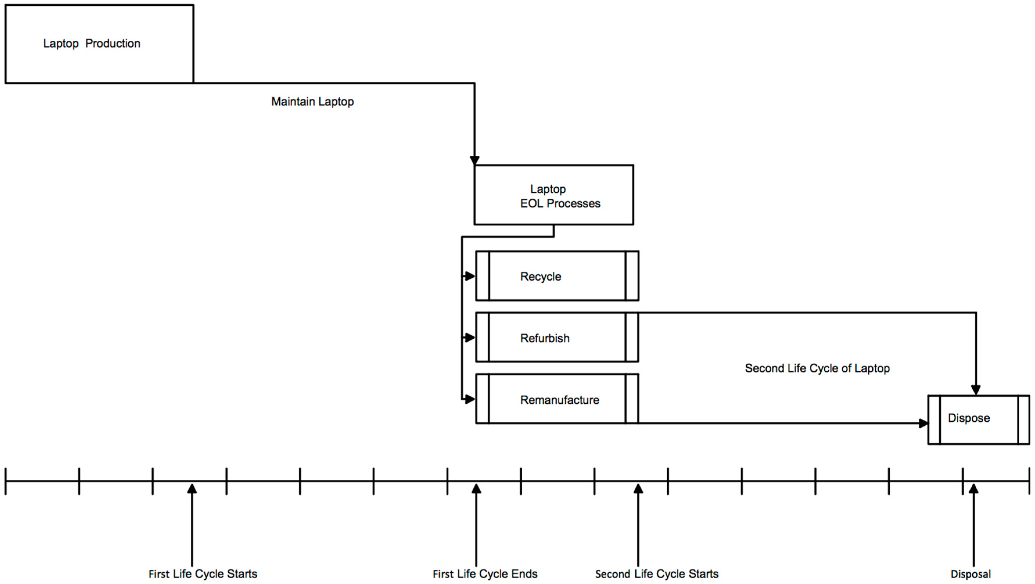
In this section, regular laptop (RL) and sensor-embedded laptop (SEL) systems are described and compared within two subsystems: maintenance operations, which affect the first life cycle of the laptops; and EOL operations, which occur during the second life cycle of the laptops. Figure 1 provides an overview of two life cycles that were modeled in this paper and the relevant operations for each cycle.
After laptops are produced and sold to the customers, the first life cycle starts. In this phase, if a laptop fails, service is provided to the customer. Once laptops complete their useful lives, they are utilized for several EOL processes such as recycling, refurbishing, and/or remanufacturing.
3.1. Maintenance of Laptops
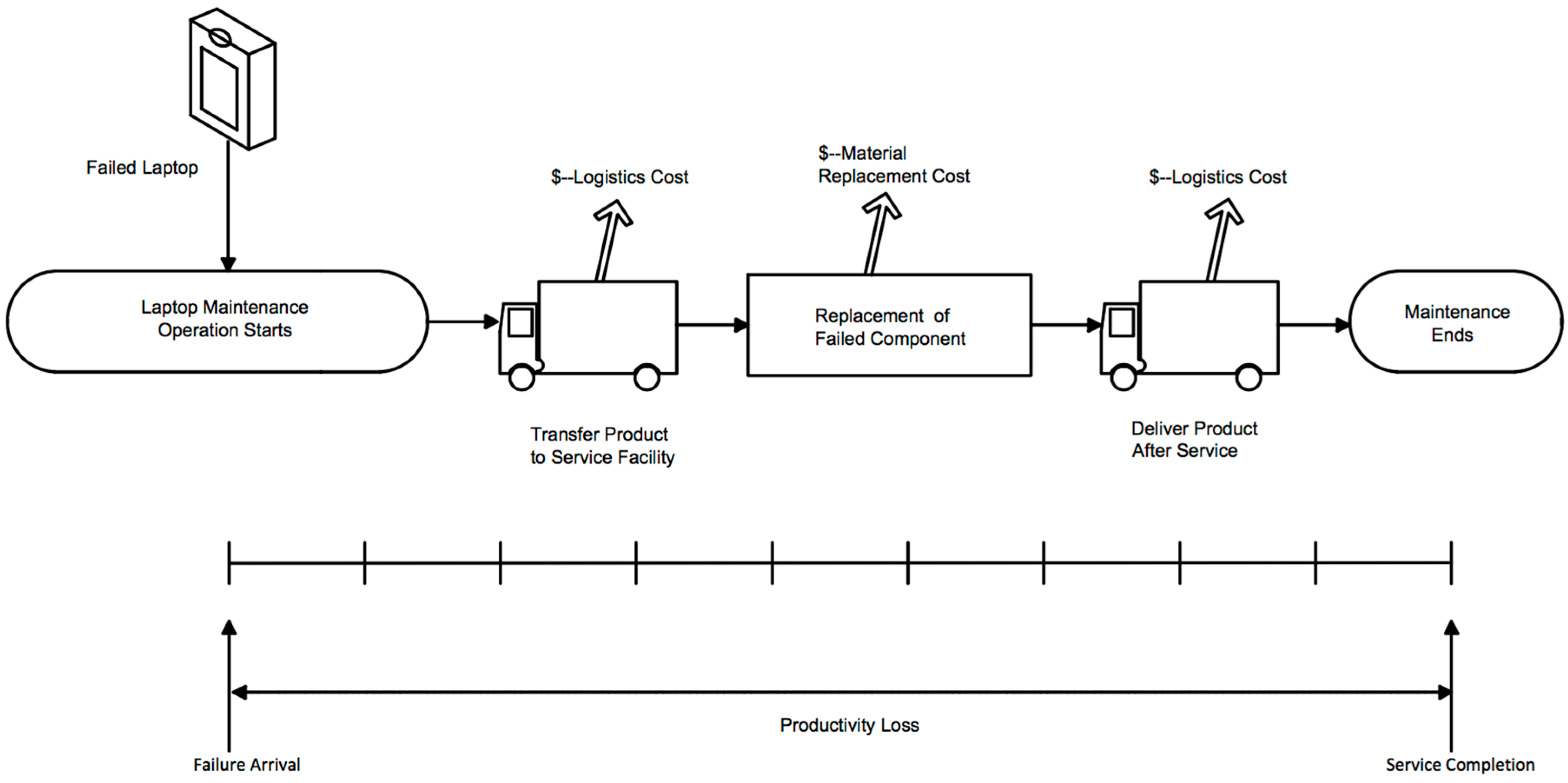
The first life cycle of the laptops involves maintenance operations. Figure 2 demonstrates the maintenance part of the systems that was considered in this study. Laptops are introduced into the system following production and sales. They have an expected usage of three years on average. RL laptops follow a corrective maintenance strategy. If they fail during their use phase, a maintenance service is provided. In this study, it was assumed that failed components are replaced with new parts as opposed to being repaired. The purpose of replacing the failed components with new ones is to increase the EOL quality of the components. Once the laptops complete their life cycles, they are sent to an EOL processing facility.
3.1.1. Maintenance of RL Systems
In RL systems, once the laptops fail, they are inspected to determine which of the components failed. The information about the failure is transmitted to the service personnel who conduct the required service operations; for example, replacing the failed component or components. These operations are represented by the recognition of failure and service activation processes, which are presented in Figure 3. After this process, failed laptops are transferred to the service facility. The replacement process takes place, and laptops are brought back to working condition. Once the service operations are complete, the products are returned to the customers.
Productivity loss occurs when laptops are not in use due to failures. In the system, productivity loss time is calculated by determining the time between the laptop failure and the service completion time. Productivity loss time incurs costs and is a function of the expected lifespan of laptops and their purchase price. Maintenance costs include the costs that are incurred as a result of inspecting the failure. Since a corrective maintenance strategy is chosen and the failed components are replaced, the material cost associated with the replacement of the components is added to the overall maintenance cost. Finally, logistics costs are also taken into consideration within maintenance costs.
3.1.2. Maintenance of SEL Systems
For SEL systems, a predictive maintenance strategy is followed. Failures can be estimated prior to failure in SEL systems since the condition information about the components can be retrieved from the embedded sensors. Inspection operation to detect the failure is not needed because sensors provide required information. By using this information, sensors can estimate the failure and send signals to the service facility to activate the maintenance service. Thus, proper actions can be taken prior to failure. As a result, recognition and service activation process in maintenance operations of RL systems is eliminated in the SEL systems. Figure 4 presents the maintenance operations of SEL systems.
Sensors can provide cost savings in SEL systems by eliminating or reducing inspection and productivity loss costs. Eliminating the inspection operation reduces labor costs. In addition, the maintenance operations required to return the laptops to full working condition can be completed in a shorter time. This will entail that the productivity loss costs are lower in SEL systems than they are in RL systems. In addition to cost saving benefits of sensors, laptops can last longer because the components that are predicted to fail are replaced with the new ones prior to failure and catastrophic failures are avoided.
3.2. Laptop EOL Processes
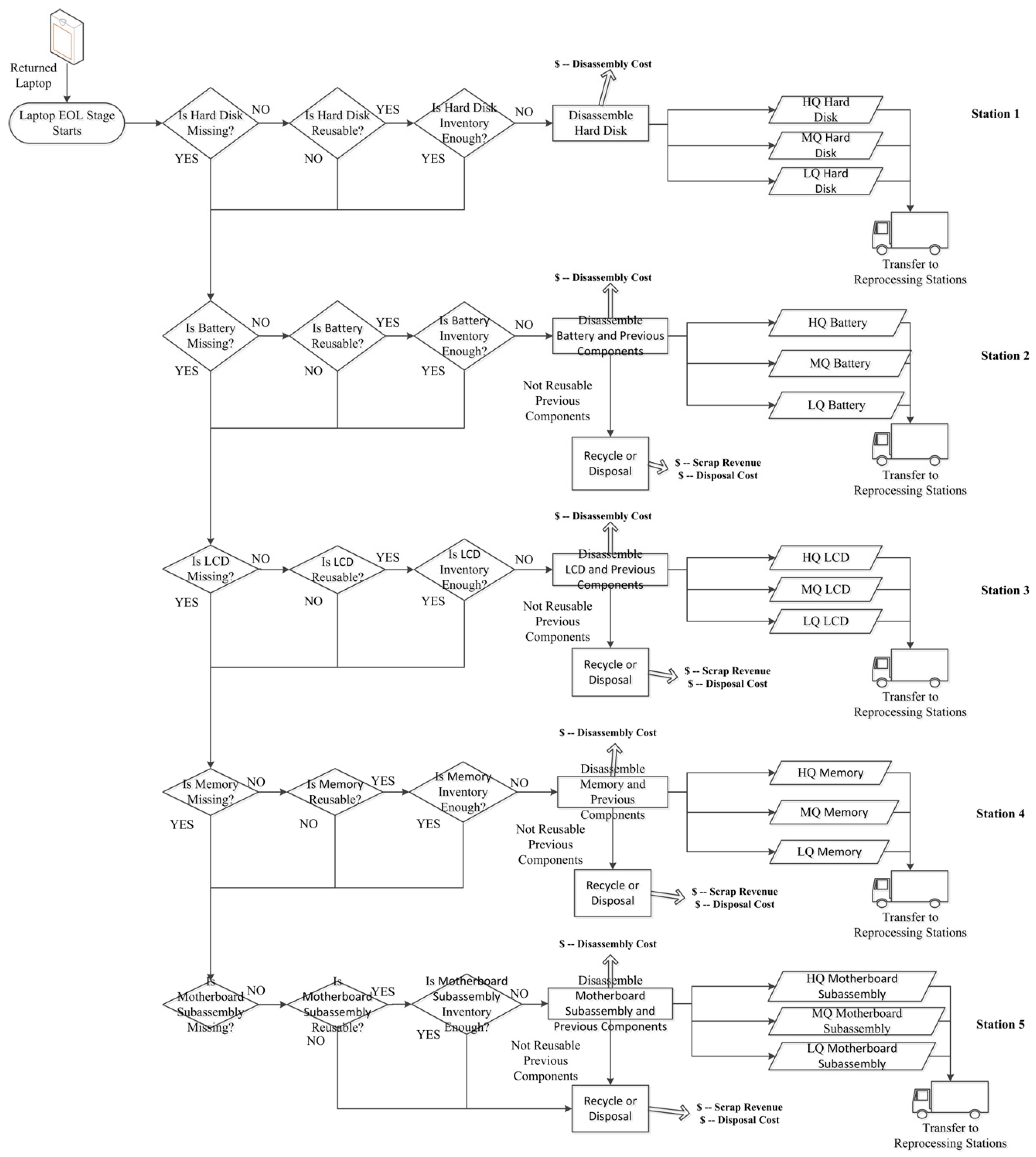
EOL processes take place after the laptops complete their useful lives. EOL laptops are sent to the facility for EOL processing. Disassembly is performed through a five-station disassembly line. Figure 5 and Figure 6 illustrate the disassembly stations that are used within RL and SEL systems. Within the model, the laptops are disassembled according to the sequence presented in Figure 5 and Figure 6.
3.2.1. Disassembly and Inspection Operations of RL Systems
In RL systems, components are disassembled via a disassembly line that follows the given sequence unless they are missing. If a component is missing, the laptop is sent to the next station. The disassembly cost is the function of labor cost and the time required to disassemble the components. As mentioned in the previous sections, inspection follows the disassembly process and is necessary for determining the reusability and quality levels of the components. The inspection costs differ according to inspection time, labor cost, and machining cost. After the inspection process, EOL processes are performed based on the determinations given in the component flows for each quality level. Figure 5 presents the details of EOL processes associated with RL systems that were considered in this research.
3.2.2. Disassembly and Inspection Operations of SEL Systems
The flow of EOL processes in SEL systems are depicted in Figure 6. The disassembly and inspection structure of the SEL systems are more complex than those of the RL systems. Using the information provided by the sensors, the EOL processes can be planned differently.
In the case of SEL, missing components have already been identified prior to disassembly; as such, laptops are transferred to the following station without visiting the station associated with that missing component. If the components are not missing, reusability information is retrieved from the sensors, and the flow is determined based on this information. If they are not reusable, they are not disassembled and sent to the next station. If the other component at the next station requires disassembly, they are disassembled together. Disassembly costs can be reduced by disassembling the reusable and non-reusable components together at the same station. This is not applicable in the RL system because components require manual inspection at the stations. If the components are reusable, the inventory levels are checked for each quality level. If the number of components has not reached maximum inventory levels, they are disassembled and sent to the reprocessing area. Otherwise, they are sent to the next station. If the other component at the next station requires disassembly, they are disassembled together. An upfront inventory check can reduce both the disassembly and inventory costs.
3.2.3. Reprocessing Operations
The quality levels of the components are divided into categories, such as high-quality (HQ), medium-quality (MQ), and low-quality (LQ) components in RL and SEL systems. The expected lifespan of HQ components is between two and three years. MQ components last for between 12 months to two years, and LQ components can last about six months up to one year. Disassembled and inspected components that have quality labels attached to them are transferred to the reprocessing area. The flows of these components are different for each quality level.
The HQ-component flow includes each quality level in the flow. If the maximum HQ remanufactured laptop inventory level is not reached in the system, HQ components are sent to the HQ remanufacturing buffer area. Otherwise, the maximum HQ component inventory is checked for component sale. If the maximum HQ component inventory level is reached, HQ components are sent for use in MQ processes instead of being recycled because they can increase the quality of the MQ level either by using them for remanufacturing or selling them as components. A similar flow can be observed in the MQ level. If the HQ components are not required at the MQ level, they can be used at the LQ level. If none of the options are chosen, HQ components are recycled or disposed of based on the materials they contain. Figure 7 depicts the HQ component flow.
Based on the flow, if the components are sold, they generate revenue for the system, and this is added to sales revenue. If they are not remanufactured or sold as used components, they are recycled, and scrap revenue is generated. If they are not recyclable, disposing of them will increase the disposal cost of the systems.
The MQ-component flow is like the HQ component flow with one exception: the MQ components are not sent to the upper level for replacement. They are sent to the LQ level for replacement if they are not used at the MQ level. The LQ-component flow only considers the flow of LQ-level components without replacement with components of a higher quality.
The components are renewed when they fail and the renewal time of the components is tracked in the systems. Based on this, the time that the components have been in use can be calculated and used to estimate quality of the components when they are disassembled at the end of products’ life cycles. In the study, it was assumed that if the components of laptops are in use for more than 1.5 years, their expected quality levels are lower, and their chance of reuse decreases.
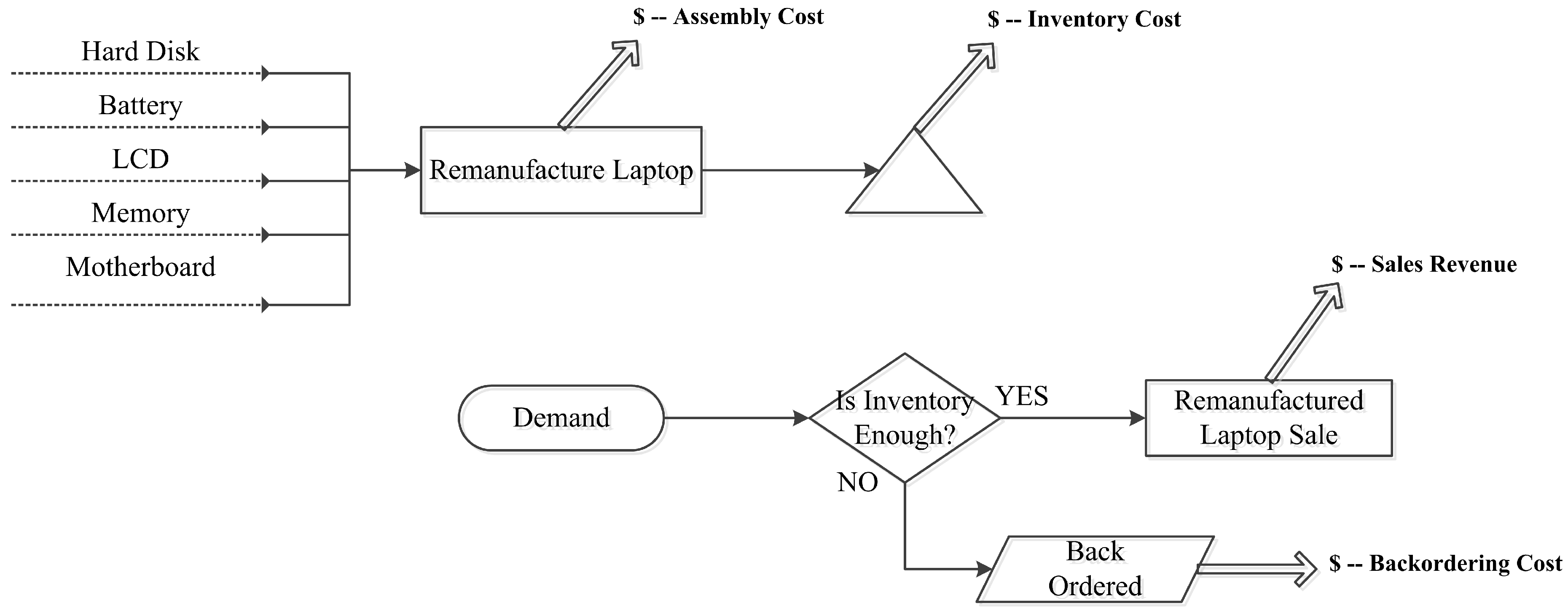
If the remanufacturing option is chosen in these component flows, the components are sent to the remanufacturing buffer area, as previously mentioned. Figure 8 shows the buffer area for each of the components of a laptop. They wait in the buffer area until one component from each component type is available. Once the component package is complete, they are assembled to remanufacture a laptop. The system costs increase relative to the assembly costs associated with remanufacturing laptops. The remanufactured laptops are added to the remanufactured laptop inventory. If there is demand, they are sold. Otherwise, they remain in the inventory, and this increases the inventory cost.
In the current study, demand was anticipated to follow a Poisson distribution. If inventory is sufficient to fulfill the demand, remanufactured laptops are sold, and revenue is generated. If the inventory is insufficient, demand is backordered and the backordering costs in the system increase. Figure 8 reveals the remanufacturing and demand flow of the laptops and the relevant revenue and costs.
4. Design of the Experimental Study
In the current study, a design of experiments study was used to compare the SEL and RL systems. The factors that might affect the revenue and costs were determined. A total of 63 factors and a significant number of experiments were needed to produce a full factorial design. The orthogonal arrays method considers a subset of combinations of those factors and reduces the number of experiments. Using this method, 63 factors with two levels were identified in such a way that 64 experiments were carried out for both systems. The combinations of the factors can be seen in the L64(263) orthogonal array [56]. Relevant data to determine the factor levels was extracted from the study conducted by Ilgin and Gupta [40].
The remanufactured laptop and component prices applied in this study are shown in Table 1. The factorial design considered only HQ- and MQ-level prices. LQ-level prices were not considered because they have insignificant impact on performance measures.
Disassembly is an essential process that can be improved by efficiently utilizing the data provided by sensors. Disassembly-related factors, such as time taken to disassemble the components and the disassembly costs, were considered in the factorial design. These factors and their levels are shown in Table 2.
Table 3 presents the inspection-related factors that were assessed in the current study: component inspection time and costs.
In the current study, missing components, component reusability, and the conditions of the components followed probability distributions, and each of these was deemed to have a direct impact on the number of remanufactured laptops and the number of components that were sold. These measures are also directly related to revenue; therefore, they were considered as factors and included in the factorial design of the study. Condition information of the components is employed in three categories such as HQ, MQ, and LQ levels. Total probability of retrieving HQ-, MQ-, and LQ-level components is equal to 1. For example, if HQ- and MQ-level probability levels are set at 0.5 and 0.3, respectively, LQ-level probability is calculated by subtracting the sum of 0.5 and 0.3 from 1. Thus, in this case, the LQ-level probability will be 0.2. This allows that once HQ- and MQ-level probabilities are identified in the experiments, LQ-level probabilities could be determined. As a result, only HQ- and MQ-level probabilities are included in the factorial design. Table 4 presents probability levels used in the factorial design. Table 5 shows LQ-level probabilities which are excluded in the factorial design.
In addition to the probabilities defined in Table 4 and Table 5, Table 6 shows another level of probabilities that were applied when the renewal-time threshold of 1.5 years was exceeded. It was assumed that, if a component had been in use for more than 1.5 years, retrieving it in HQ condition was less likely; as such, the probability of this occurring was reduced by 0.3.
The maintenance costs of the systems modeled in the current study consisted of several subcategory costs such as labor cost, productivity loss cost, material replacement cost, and logistics costs. Some of the factors that might make difference between SEL and RL systems were considered in the factorial design and can be observed in Table 7. The time taken to recognize the problem and activate the laptop service was among them. In addition, the time at which the failure was inspected was also included, and it was assumed that this followed a normal distribution. The mean and standard deviation values of the normal distribution are presented in the parenthesis in Table 7.
Demand represents an important consideration among the factors because, if there is a demand, producers can generate revenue by selling remanufactured laptops and disassembled components. HQ- and MQ-level demands were considered in the factorial design and were assumed to follow a Poisson distribution. The average daily rates for both levels that were applied are shown in Table 8. As was the case with the LQ-prices, the LQ-level demands were not included in the factorial design.
In the SEL and RL systems, the failure of a component might cause defects in the other components. There is a rate for this measure, and this was included in the factorial design. In addition, the remanufacturing process involves an assembly operation by which the disassembled components are reassembled. The assembly cost and assembly time were of relevance within this process and were considered in the factorial design. These three factors can be seen in Table 9.
Discrete event simulation was used to model the RL and SEL systems. Arena 14.7 simulation software (Rockwell, Austin, TX, USA) was used for the modeling process [57]. To validate the models, they were run by assigning extreme values to variables and corresponding performance measures were observed with these runs. For example, if probability of retrieving HQ components is 1 the systems should not produce any output related to MQ and LQ components such as number of sold MQ and LQ components and remanufactured MQ and LQ laptops. The run length of the simulation experiments was 1500 days, which is approximately 4 years. After a laptop had completed its expected life span of three years, the models were run over the duration of one more year for EOL operations. A total of 63 factors were used within the factorial design, and these were described in this section. The data that were not included in the factorial design, but were required to run the experiments, are shown in Table A1, Table A2, Table A3, Table A4, Table A5, Table A6 and Table A7.
SEL and RL systems were introduced, and the design of experiments study was explained. The purpose of this study was to determine whether SEL systems can substantially increase EOL profit and reduce maintenance costs in comparison to RL systems. The performance measures that were used to calculate this amount is shown below.
5. Results and Analysis
For each system, RL and SEL, experiments were carried out, and the data pertaining to the EOL profit per laptop, maintenance cost per laptop, total profit, disassembly cost, and inspection costs were tracked.
The average value of EOL profit per laptop was $203.30 for the SEL system and $190.59 for the RL system. These profits were generated by EOL processes, such as recycling, resale, and remanufacturing. Another important measure that is of significance to sensor value is the maintenance cost. In the SEL systems, the maintenance cost per laptop was, on average, $56.94. In RL systems, it was $60.31. Maintaining laptops throughout their life cycles incurs these costs in both systems.
The data indicated that the use of sensors significantly reduced the cost of the inspection process. In RL systems, the inspection cost for the simulation period was $107,274.80 while this reduced to $1264.20 in the SEL systems. The disassembly costs were $83,127.33 and $90,726.56 for the SEL and RL systems, respectively. Table 10 presents the average values of the performance measures mentioned above, as well as the total profit for both systems.
A pairwise t-test was used to determine if the difference between the RL and SEL systems was statistically significant. A factorial design with orthogonal arrays corresponding to unique factors for each experiment was employed; as such, the experiments were paired. The results of the pairwise t-tests, including mean differences and p-values, are presented in Table 11.
The test results for the EOL profit per laptop value indicated that the mean difference between the two systems was $13.20 in favor of the SEL systems. The p-value presented in Table 11 was less than 0.0001 and reveals that the EOL profit difference between the systems was statistically significant. Furthermore, the mean value of the maintenance cost difference between the systems was $−3.38. This indicates that the use of the SEL system as opposed to the RL system generated a cost saving of $3.38. The t-test results for the other performance measures, such as total profit, disassembly cost, and inspection cost, are presented in Table 11.
The sensor value is the sum of EOL profit improvement and maintenance cost savings and, in the study, was calculated to be $16.09. It can, therefore, be concluded that it is worthwhile embedding sensors in laptops if the cost of these sensors is below $16.09 per unit. In addition to the mean differences and p-values, 95% confidence in the mean difference of the measures was achieved, as per the data presented in Table 12.
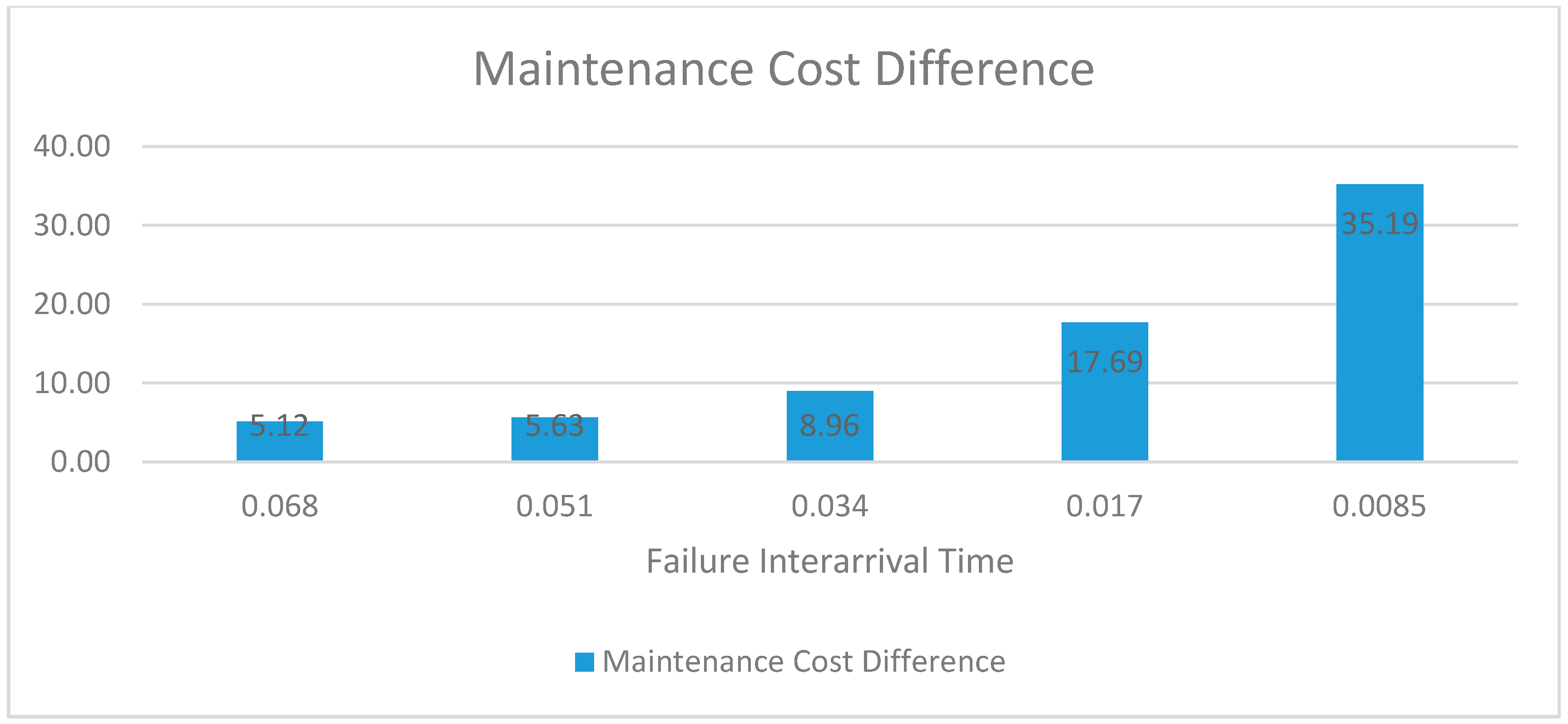
In the study, failures were assumed to arrive into the system at exponential interarrival times. A total of 63 factors were used in the design of experiments, and failure interarrival times were not considered as a factor. Further runs were taken to determine the impact of different interarrival times on the maintenance cost and sensor value. Figure 9 presents the maintenance costs of the systems if interarrival times are reduced; namely, failure rate increases. The maintenance cost increased with the reduction of failure interarrival times, and a negative correlation between the failure interarrival times and the maintenance costs was observed.
In addition, differences between the two systems in terms of maintenance costs also had a negative correlation with the failure interarrival times. Figure 10 presents information related to the increase in maintenance costs that were observed when the failure interarrival times were reduced.
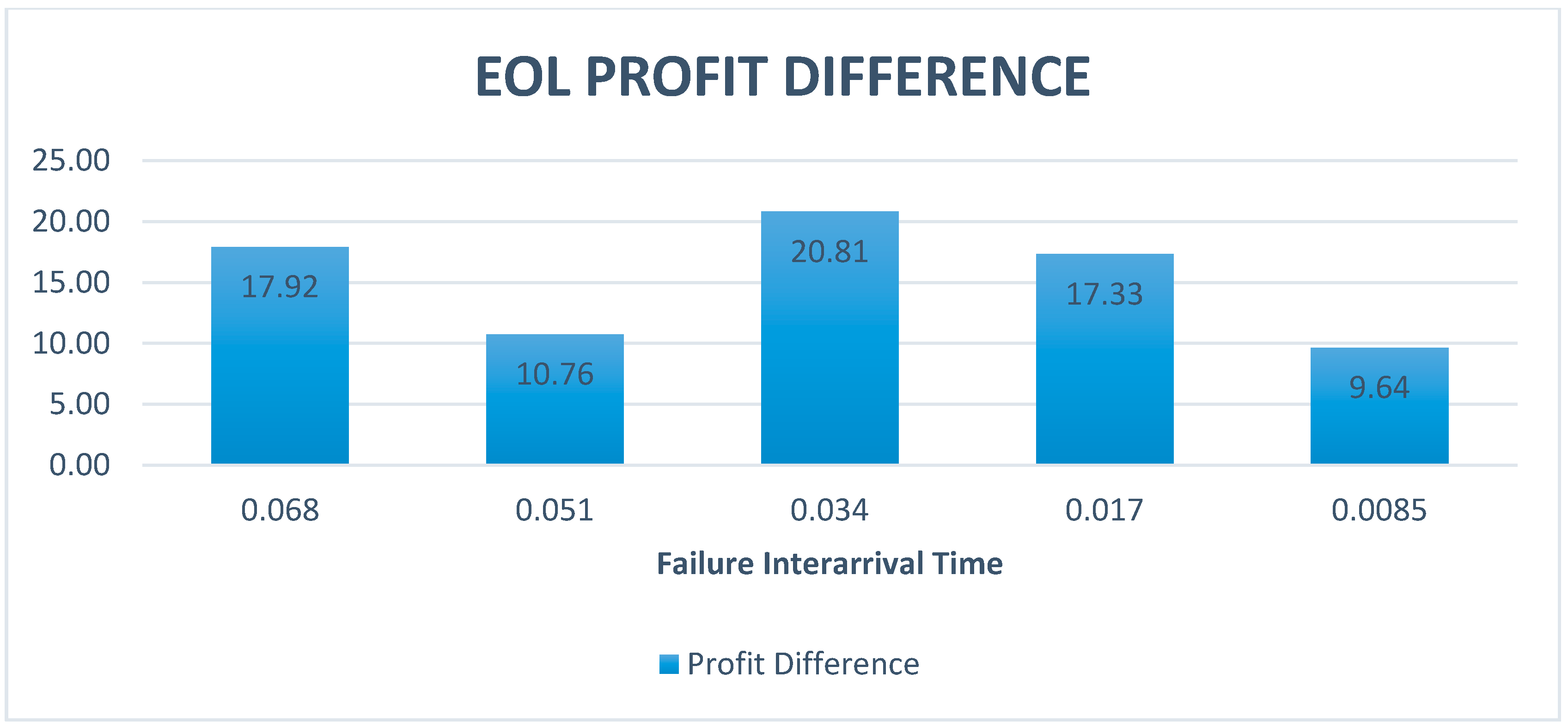
Furthermore, Figure 11 demonstrates the relationship between the EOL profit difference between the systems and the failure interarrival times. A failure interarrival rate reduction from 0.068 to 0.051 had a negative impact on the profit difference because the quality of the returned components decreased. However, when the failure interarrival time was 0.034, the profit difference increased. This can be attributed to the renewal time consideration in the system. It was assumed that if laptops fail more frequently, it is more likely that most of the components will be renewed and their EOL quality will be higher. This will lead to higher EOL profit. The best scenario for EOL profit among all the failure interarrival times was 0.034.
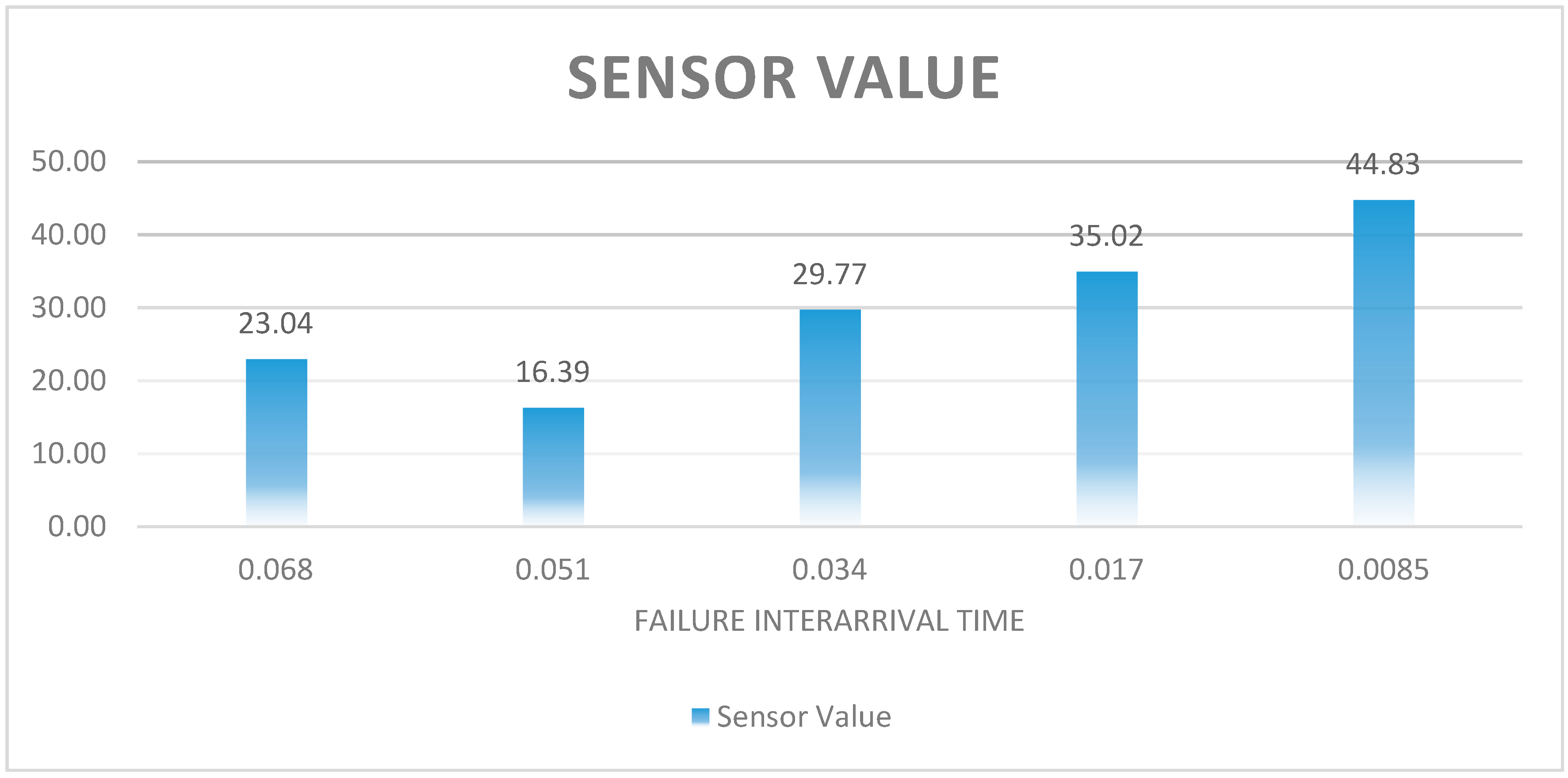
Finally, Figure 12 presents the impact of the failure interarrival times on the overall sensor value. The best scenario for the sensor value was 0.0085.
6. Conclusions
SEL systems performed better than RL systems in terms of the maintenance cost of the systems and the EOL profit that the systems generated. The information about the conditions of the components is of particular relevance because it can be used to gain an economic advantage in a closed-loop supply chain system. The maintenance cost of the system can be reduced, on average, by $3.38. Furthermore, the disassembly costs that are incurred in the SEL system were calculated to be $7599.23 less than the disassembly costs in the RL system for the simulation period. The inspection cost saving is higher than the disassembly cost saving and is $106,010.60. These savings increase the total profit of the SEL system by $123,181.10. The overall sensor value was calculated to be $16.09.
Our results illustrate that firms can invest in remote monitoring technologies, such as sensors, and increase the profit that they make out of selling EOL products and their components, as well as decrease the maintenance cost of the products during their life cycles. Beyond their financial benefits, sensors can provide enhanced visibility through the supply chain because they allow remote and simultaneous tracking. This can result in improved supply and inventory planning. This study examined the use of sensors to enhance the performance of maintenance activities and EOL operations of the returned products. They can also be helpful in reducing the inventory costs. Future research could examine this benefit financially.
In this study, it was discussed that sensors will be embedded into laptops and provide condition information about them through their lifecycles. It was assumed that sensors would give accurate estimations about the condition and they would not fail during this time period. This study can be expanded by employing the reliability of the sensors. It is critical that they should provide accurate information because replacing some of the components can be costly and this would exceed even the cost savings gained during the maintenance stage.
Acknowledgments
The authors would like to thank the reviewers for their insightful comments and feedback to enhance the quality of this article.
Author Contributions
M.T.D. reviewed the relevant literature to conduct this study. He developed the simulation models and performed the experiments. S.M.G. determined the research direction and provided guidance during the development of the research idea. Both authors reviewed the experimental results and drew conclusions about the research.
Conflicts of Interest
The authors declare no conflict of interest.
Appendix A

Table A1.
Low-quality remanufactured laptop, subassembly, and component prices.
| LQ Laptop ($) | 200 |
| LQ Hard Disk ($) | 25 |
| LQ Battery ($) | 20 |
| LQ LCD ($) | 50 |
| LQ Memory ($) | 10 |
| LQ Motherboard ($) | 50 |
Table A2.
Low-quality remanufactured laptop, subassembly, and component demands.
| (Follows Poisson Distribution) | |
|---|---|
| LQ Laptop (day) | 50 |
| LQ Hard Disk (day) | 50 |
| LQ Battery (day) | 50 |
| LQ LCD (day) | 50 |
| LQ Memory (day) | 50 |
| LQ Motherboard (day) | 50 |
Table A3.
Maintenance data.
| Failure Arrival Rate (Day) (Exponentially Distributed) | 0.068 |
| Expected Lifetime (year) | 3 |
| Transportation Before Service (day) | 1 |
| Delivery After Service (day) (Triangular Distribution) | Min (1), Mean (2), Max (3) |
| Transportation Cost ($) | 5 |
| Delivery Cost ($) | 30 |
Table A4.
Subassembly and component replacement times for maintenance.
| (Normally Distributed) (Mean, Standard Deviation) | |
|---|---|
| Hard Disk (min) | (3, 0.2) |
| Battery (min) | (1, 0.1) |
| LCD (min) | (10, 0.5) |
| Memory (min) | (3, 0.4) |
| Motherboard (min) | (10, 0.5) |
Table A5.
Subassembly and component replacement costs for maintenance.
| Hard Disk ($) | 150 |
| Battery ($) | 100 |
| LCD ($) | 240 |
| Memory ($) | 60 |
| Motherboard ($) | 300 |
Table A6.
Subassembly and component failure probabilities.
| Component | % |
|---|---|
| Hard Disk Failure | 25 |
| Battery Failure | 15 |
| LCD Failure | 25 |
| Memory Failure | 5 |
| Motherboard Failure | 30 |
Table A7.
Production and cost data.
| Laptop Arrival Rate (min) (Exponentially Distributed) | 3 |
| Disposal Cost ($/lbs) | 0.4 |
| Scrap Revenue ($/lbs) | 0.6 |
| Metal Recycle Rate | 0.3 |
| Holding Cost Rate | 0.2 |
| Backordering Cost Rate | 0.6 |
References
- Govindan, K.; Soleimani, H.; Kannan, D. Reverse logistics and closed-loop supply chain: A comprehensive review to explore the future. Eur. J. Oper. Res. 2015, 240, 603–626. [Google Scholar] [CrossRef] [Green Version]
- Walker, W.T. Rethinking the reverse supply chain. Supply Chain Man. Rev. 2000, 4, 52–59. [Google Scholar]
- Chen, W.; Kucukyazici, B.; Verter, V.; Sáenz, M.J. Supply chain design for unlocking the value of remanufacturing under uncertainty. Eur. J. Oper. Res. 2015, 247, 804–819. [Google Scholar] [CrossRef]
- Das, K.; Posinasetti, N.R. Addressing environmental concerns in closed loop supply chain design and planning. Int. J. Prod. Econ. 2015, 163, 34–47. [Google Scholar] [CrossRef]
- Sgarbossa, F.; Russo, I. A proactive model in sustainable food supply chain: Insight from a case study. Int. J. Prod. Econ. 2017, 183, 596–606. [Google Scholar] [CrossRef]
- Aksoy, H.K.; Gupta, S.M. Buffer allocation plan for a remanufacturing cell. Comput. Ind. Eng. 2005, 48, 657–677. [Google Scholar] [CrossRef]
- Ilgin, M.A.; Gupta, S.M. Environmentally conscious manufacturing and product recovery (ECMPRO): A review of the state of the art. J. Environ. Manag. 2010, 91, 563–591. [Google Scholar] [CrossRef] [PubMed]
- Giglio, D.; Paolucci, M.; Roshani, A. Integrated lot sizing and energy-efficient job shop scheduling problem in manufacturing/remanufacturing systems. J. Clean. Prod. 2017, 148, 624–641. [Google Scholar] [CrossRef]
- Quariguasi-Frota-Neto, J.; Bloemhof, J. An analysis of the Eco-Efficiency of remanufactured personal computers and mobile phones. Prod. Oper. Manag. 2012, 21, 101–114. [Google Scholar] [CrossRef]
- Abbey, J.D.; Meloy, M.G.; Guide, V.D.R.; Atalay, S. Remanufactured products in closed-loop supply chains for consumer goods. Prod. Oper. Manag. 2015, 24, 488–503. [Google Scholar] [CrossRef]
- Wang, W.; Wang, Y.; Mo, D.; Tseng, M.M. Managing component reuse in remanufacturing under product diffusion dynamics. Int. J. Prod. Econ. 2017, 183, 551–560. [Google Scholar] [CrossRef]
- Colledani, M.; Copani, G.; Tolio, T. De-manufacturing systems. Procedia CIRP 2014, 17, 14–19. [Google Scholar] [CrossRef] [Green Version]
- Moore, K.E.; Güngör, A.; Gupta, S.M. Petri net approach to disassembly process planning for products with complex AND/OR precedence relationships. Eur. J. Oper. Res. 2001, 135, 428–449. [Google Scholar] [CrossRef]
- Kim, H.J.; Lee, D.H.; Xirouchakis, P. Disassembly scheduling: Literature review and future research directions. Int. J. Prod. Res. 2007, 45, 4465–4484. [Google Scholar] [CrossRef]
- Morgan, S.D.; Gagnon, R.J. A systematic literature review of remanufacturing scheduling. Int. J. Prod. Res. 2013, 51, 4853–4879. [Google Scholar] [CrossRef]
- Gupta, S.M.; Taleb, K.N. Scheduling disassembly. Int. J. Prod. Res. 1994, 32, 1857–1866. [Google Scholar] [CrossRef]
- Taleb, K.N.; Gupta, S.M. Disassembly of multiple product structures. Comput. Ind. Eng. 1997, 32, 949–961. [Google Scholar] [CrossRef]
- Taleb, K.N.; Gupta, S.M.; Brennan, L. Disassembly of complex product structures with parts and materials commonality. Prod. Plan. Control 1997, 8, 255–269. [Google Scholar] [CrossRef]
- Lee, D.H.; Xirouchakis, P. A two-stage heuristic for disassembly scheduling with assembly product structure. J. Oper. Res. Soc. 2004, 55, 287–297. [Google Scholar] [CrossRef]
- Barba-Gutierrez, Y.; Adenso-Diaz, B.; Gupta, S.M. Lot sizing in reverse MRP for scheduling disassembly. Int. J. Prod. Econ. 2008, 111, 741–751. [Google Scholar] [CrossRef]
- Habibi, M.K.; Battaïa, O.; Cung, V.D.; Dolgui, A. Collection-disassembly problem in reverse supply chain. Int. J. Prod. Econ. 2017, 183, 334–344. [Google Scholar] [CrossRef]
- Jeihoonian, M.; Zanjani, M.K.; Gendreau, M. Accelerating Benders decomposition for closed-loop supply chain network design: Case of used durable products with different quality levels. Eur. J. Oper. Res. 2016, 251, 830–845. [Google Scholar] [CrossRef]
- Duffuaa, S.; Raouf, A. Planning and Control of Maintenance Systems: Modelling and Analysis; Springer: Berlin, Germany, 2015. [Google Scholar]
- Olanrewaju, A.L.; Abdul-Aziz, A.R. Building Maintenance Processes and Practices; Springer: Berlin, Germany, 2015. [Google Scholar]
- Hashemian, H.M. Wireless sensors for predictive maintenance of rotating equipment in research reactors. Ann. Nucl. Energy 2011, 38, 665–680. [Google Scholar] [CrossRef]
- Vijay Kumar, E.; Chaturvedi, S.K.; Deshpandé, A.W. Maintenance of industrial equipment: Degree of certainty with fuzzy modelling using predictive maintenance. Int. J. Qual. Reliab. Manag. 2009, 26, 196–211. [Google Scholar] [CrossRef]
- Angeles, R. RFID technologies: Supply-chain applications and implementation issues. Inf. Syst. Manag. 2005, 22, 51–65. [Google Scholar] [CrossRef]
- Bose, I.; Ngai, E.W.; Teo, T.S.; Spiekermann, S. Managing RFID projects in organizations. Eur. J. Inf. Syst. 2009, 18, 534–540. [Google Scholar] [CrossRef]
- Dutta, A.; Lee, H.L.; Whang, S. RFID and operations management: Technology, value, and incentives. Prod. Oper. Manag. 2007, 16, 646–655. [Google Scholar] [CrossRef]
- Dutta, A.; Whang, S. Radiofrequency identification applications in private and public sector operations: Introduction to the special issue. Prod. Oper. Manag. 2007, 16, 523–524. [Google Scholar] [CrossRef]
- Dai, F.F.; Stroud, C.E.; Zhang, J.B. Guest editorial. IEEE Trans. Ind. Electron 2009, 56, 2295–2298. [Google Scholar] [CrossRef]
- Madni, A.M.; Chalasani, S.; Boppana, R.V. Guest editorial RFID technology: Opportunities and challenges. IEEE Syst. J. 2007, 2, 78–81. [Google Scholar] [CrossRef]
- Ngai, E.; Riggins, F. RFID: Technology, applications, and impact on business operations. Int. J. Prod. Econ. 2008, 112, 507–509. [Google Scholar] [CrossRef]
- Ngai, E.W.T. Guest editorial: RFID technology and applications in production and supply chain management. Int. J. Prod. Res. 2010, 48, 2481–2483. [Google Scholar] [CrossRef]
- Vadde, S.; Kamarthi, S.; Gupta, S.M.; Zeid, I. Product life cycle monitoring via embedded sensors. In Environment Conscious Manufacturing; Gupta, S.M., Lambert, A.J.D., Eds.; CRC Press: Boca Raton, FL, USA, 2008; pp. 91–103. [Google Scholar]
- Petriu, E.M.; Georganas, N.D.; Petriu, D.C.; Makrakis, D.; Groza, V.Z. Sensor-based information appliances. Instrum. Meas. Mag. 2000, 3, 31–35. [Google Scholar]
- Borriello, G. Introduction. Comm. ACM 2005, 48, 34–37. [Google Scholar] [CrossRef]
- Ilgin, M.A.; Gupta, S.M. Comparison of economic benefits of sensor embedded products and conventional products in a multi-product disassembly line. Comput. Ind. Eng. 2010, 59, 748–763. [Google Scholar] [CrossRef]
- Ilgin, M.A.; Gupta, S.M. Evaluating the impact of sensor-embedded products on the performance of an air conditioner disassembly line. Int. J. Adv. Manuf. Technol. 2011, 53, 1199–1216. [Google Scholar] [CrossRef]
- Ilgin, M.A.; Gupta, S.M. Performance improvement potential of sensor embedded products in environmental supply chains. Resour. Conserv. Recycl. 2011, 55, 580–592. [Google Scholar] [CrossRef]
- Ilgin, M.A.; Gupta, S.M. Recovery of sensor embedded washing machines using a multi-kanban controlled disassembly line. Robot. Comput. Integr. Manuf. 2011, 27, 318–334. [Google Scholar] [CrossRef]
- Ilgin, M.A.; Gupta, S.M.; Nakashima, K. Coping with disassembly yield uncertainty in remanufacturing using sensor embedded products. J. Remanuf. 2011, 1, 1–14. [Google Scholar] [CrossRef] [Green Version]
- Ilgin, M.A.; Ondemir, O.; Gupta, S.M. An approach to quantify the financial benefit of embedding sensors into products for end-of-life management: A case study. Prod. Plan. Control 2014, 25, 26–43. [Google Scholar] [CrossRef]
- Ondemir, O.; Gupta, S.M. Optimal management of reverse supply chains with sensor-embedded end-of-life products. In Applications of Management Science; Lawrence, K.D., Kleinman, G., Eds.; Emerald Group Publishing Limited: Bingley, UK, 2012; pp. 109–129. [Google Scholar]
- Ondemir, O.; Ilgin, M.A.; Gupta, S.M. Optimal end-of-life management in closed-loop supply chains using RFID and sensors. IEEE Trans. Ind. Inf. 2012, 8, 719–728. [Google Scholar] [CrossRef]
- Ondemir, O.; Gupta, S.M. A multi-criteria decision making model for advanced repair-to-order and disassembly-to-order system. Eur. J. Oper. Res. 2014, 233, 408–419. [Google Scholar] [CrossRef]
- Ondemir, O.; Gupta, S.M. Advanced remanufacturing-to-order and disassembly-to-order system under demand/decision uncertainty. In Reverse Supply Chains: Issues and Analysis; Gupta, S.M., Ed.; CRC Press: Boca Raton, FL, USA, 2013; pp. 203–228. [Google Scholar]
- Ondemir, O.; Gupta, S.M. Quality assurance in remanufacturing with sensor embedded products. In Quality Management in Reverse Logistics; Nikolaidis, Y., Ed.; Springer: London, UK, 2013; pp. 95–112. [Google Scholar]
- Ondemir, O.; Gupta, S.M. Quality management in product recovery using the Internet of Things: An optimization approach. Comput. Ind. 2014, 65, 491–504. [Google Scholar] [CrossRef]
- Dulman, M.T.; Gupta, S.M. Benefits of sensors in cell phone disassembly and remanufacturing. In Proceedings of the Northeast Region Decision Sciences Institute (NEDSI), Cambridge, MA, USA, 19–22 March 2015. [Google Scholar]
- Dulman, M.T.; Gupta, S.M. Use of sensors for cell phones. In Proceedings of the Production and Operations Management Society (POMS), Orlando, FL, USA, 8–11 May 2015. [Google Scholar]
- Dulman, M.T.; Gupta, S.M. Disassembling and Remanufacturing End-of-Life Sensor Embedded Cell Phones. Innov. Supply Chain Manag. 2015, 9, 111–117. [Google Scholar] [CrossRef]
- Dulman, M.T.; Gupta, S.M. Use of sensors for collection of end-of-life products. In Proceedings of the Northeast Region Decision Sciences Institute (NEDSI), Alexandria, VA, USA, 31 March–1 April 2016. [Google Scholar]
- Alqahtani, A.Y.; Gupta, S.M. One-dimensional renewable warranty management within sustainable supply chain. Resources 2017, 6, 16. [Google Scholar] [CrossRef]
- Alqahtani, A.Y.; Gupta, S.M. Optimizing two-dimensional renewable warranty policies for sensor embedded remanufactured products. J. Ind. Eng. Manag. 2017, 10, 145. [Google Scholar] [CrossRef]
- Phadke, M.S. Quality Engineering Robust Design; Prentice Hall: Passaic River, NJ, USA, 1989. [Google Scholar]
- Kelton, D.W.; Sadowski, R.P.; Sadowski, D.A. Simulation with Arena, 4th ed.; McGraw-Hill: New York, NY, USA, 2007. [Google Scholar]
Figure 1.
Maintenance and EOL life-cycle scheme of laptops.

Figure 2.
Life cycle outlook of laptops.
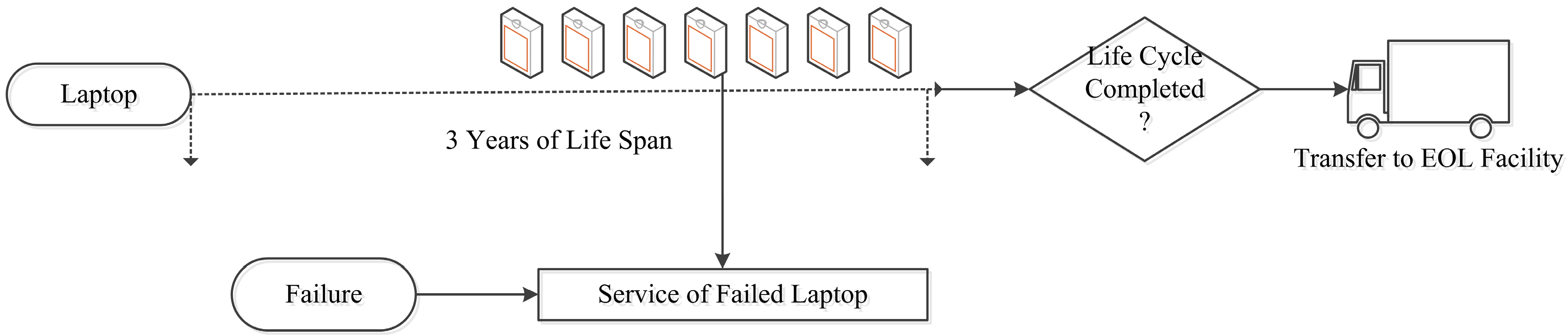
Figure 3.
Maintenance operations of RL systems.
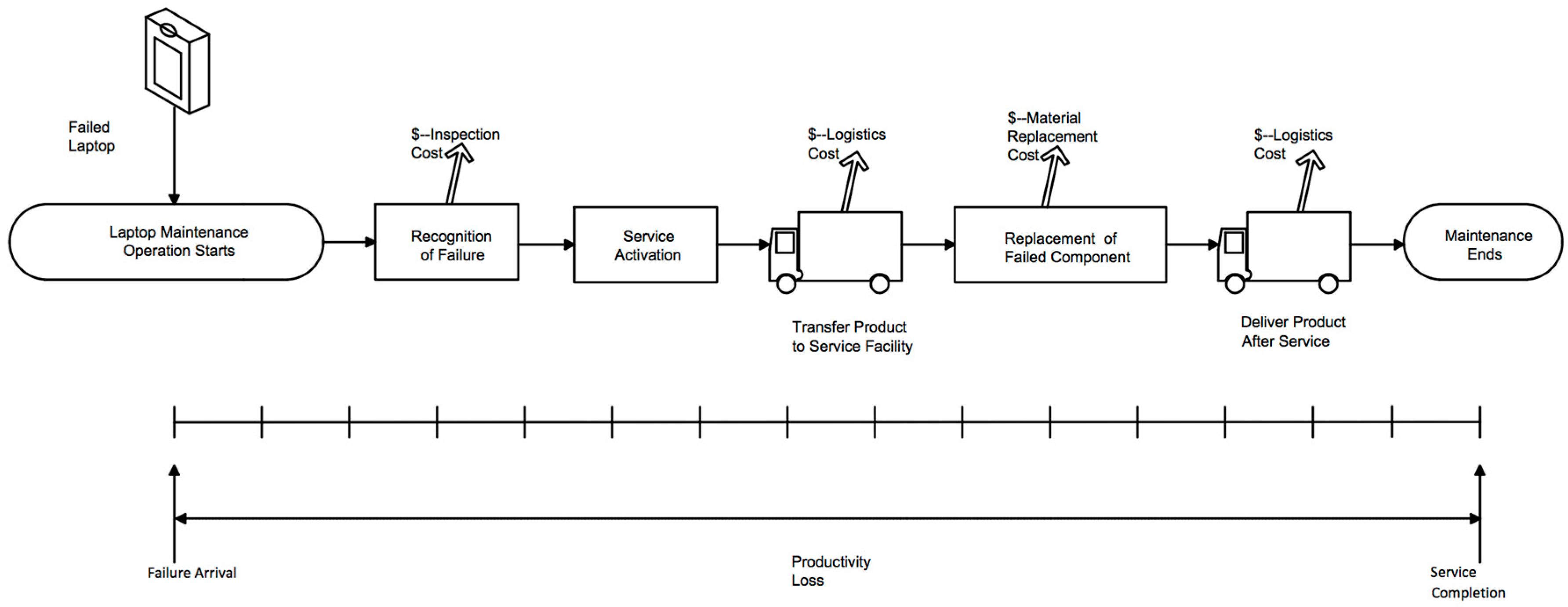
Figure 4.
Maintenance operations of SEL systems.

Figure 5.
RL systems disassembly and inspection processes.
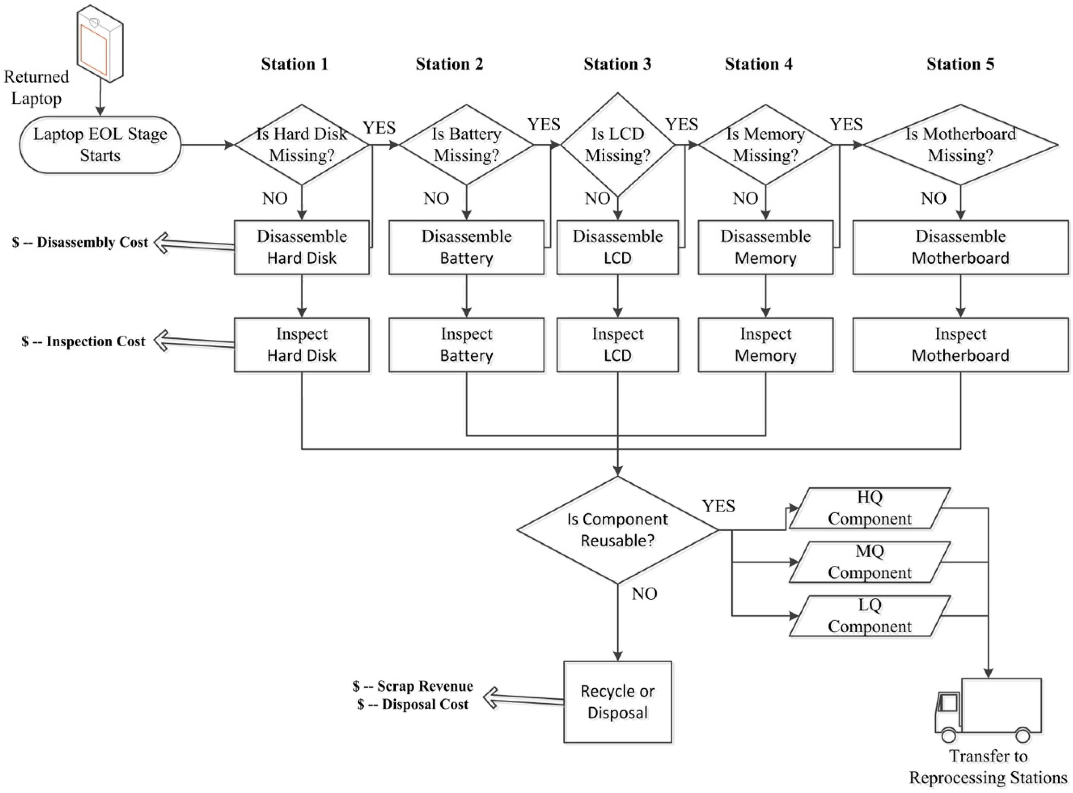
Figure 6.
SEL systems disassembly and inspection processes.

Figure 7.
HQ-component flow for recycle, resale, and remanufacturing.
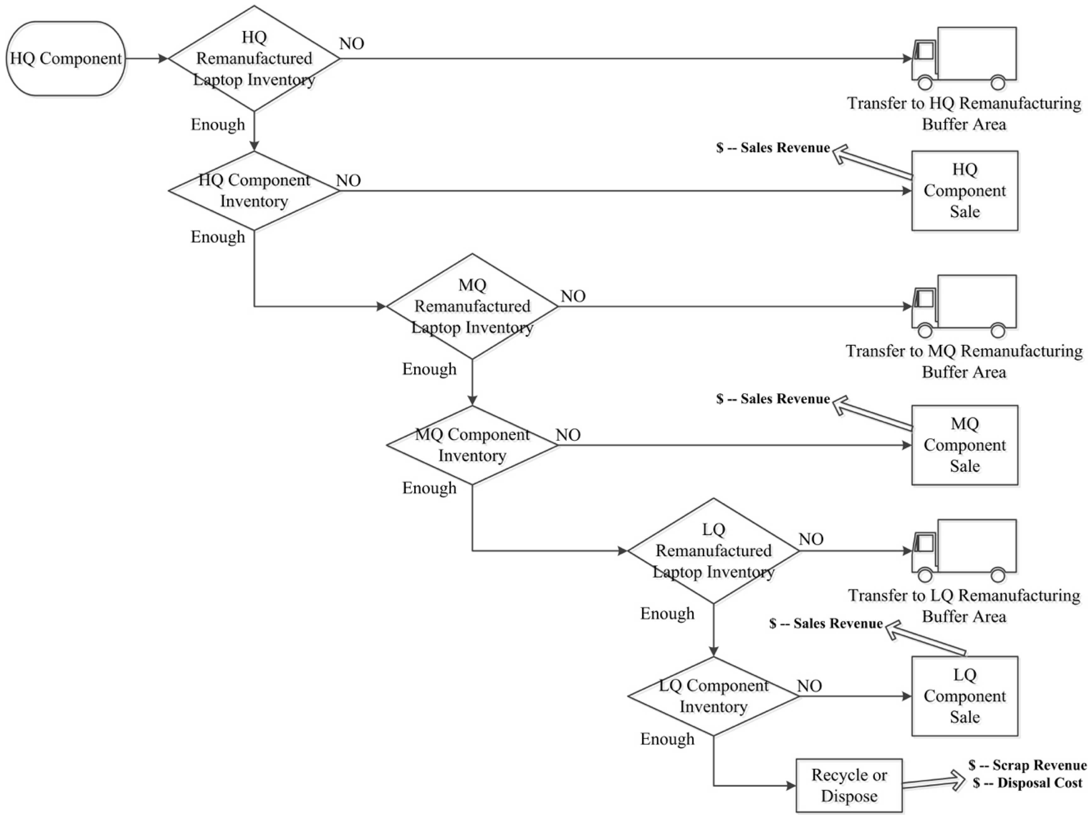
Figure 8.
Remanufacturing and demand flow of laptops.

Figure 9.
Maintenance cost of the systems.
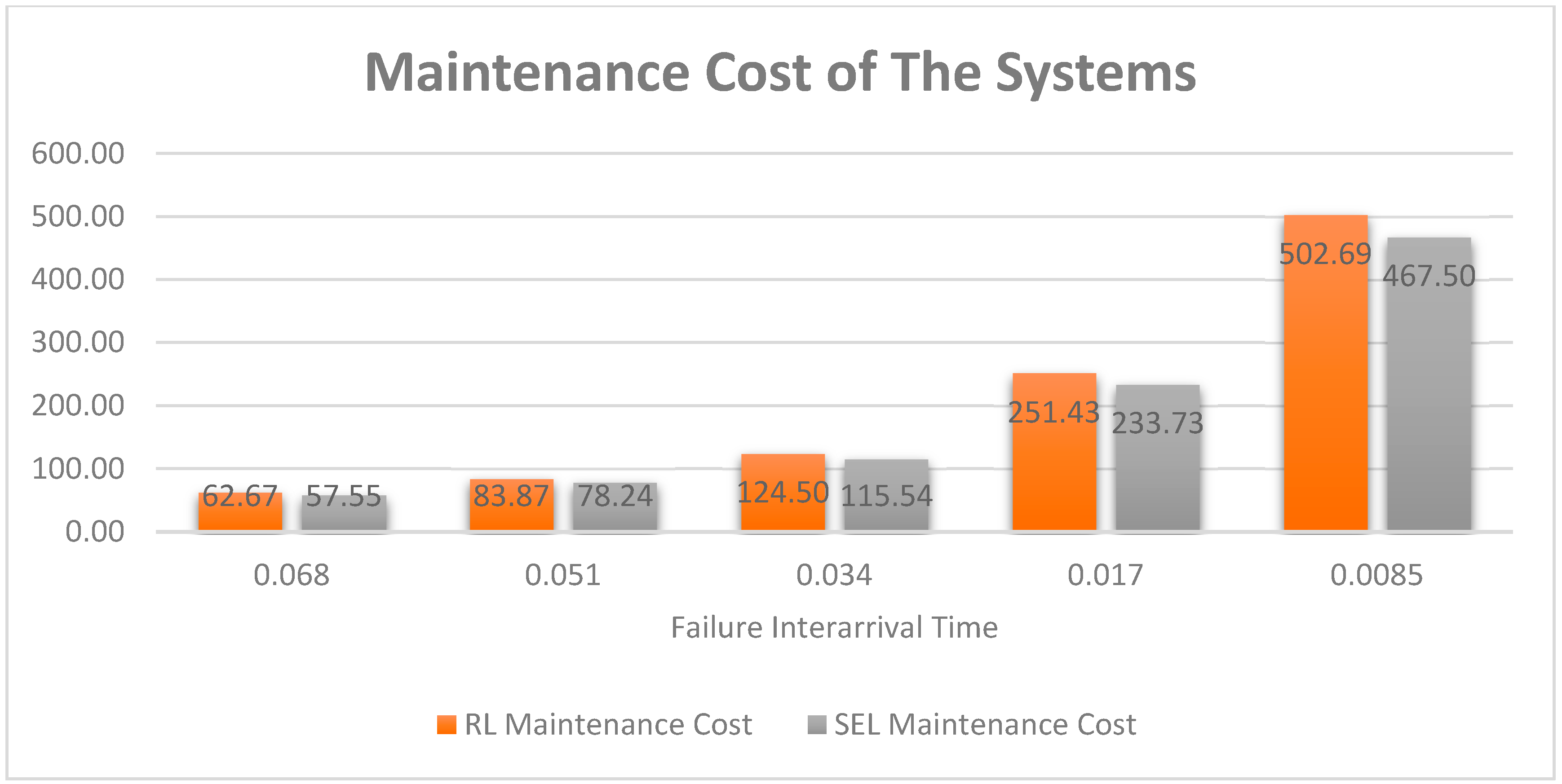
Figure 10.
Maintenance cost differences between two systems.

Figure 11.
EOL profit difference between two systems.

Figure 12.
Sensor value.

Table 1.
Remanufactured laptop, subassembly, and component prices.
| Factor | Level 1 | Level 2 |
|---|---|---|
| HQ Laptop ($) | 660 | 550 |
| HQ Hard Disk ($) | 90 | 75 |
| HQ Battery ($) | 60 | 50 |
| HQ LCD ($) | 144 | 120 |
| HQ Memory ($) | 36 | 30 |
| HQ Motherboard ($) | 180 | 150 |
| MQ Laptop ($) | 480 | 400 |
| MQ Hard Disk ($) | 60 | 50 |
| MQ Battery ($) | 48 | 40 |
| MQ LCD ($) | 96 | 80 |
| MQ Memory ($) | 24 | 20 |
| MQ Motherboard ($) | 120 | 100 |
Table 2.
Disassembly cost and time factors.
| Factor | Level 1 | Level 2 |
|---|---|---|
| Disassembly Cost ($/min) | 3 | 2 |
| Hard Disk Disassembly Time (min) | 0.9 | 0.75 |
| Battery Disassembly Time (min) | 0.6 | 0.5 |
| LCD Disassembly Time (min) | 0.9 | 0.75 |
| Memory Disassembly Time (min) | 0.6 | 0.5 |
| Motherboard Disassembly Time (min) | 1.8 | 1.5 |
Table 3.
Inspection cost and time factors.
| Factor | Level 1 | Level 2 |
|---|---|---|
| Inspection Cost ($/min) | 0.6 | 0.5 |
| Hard Disk Inspection Time (min) | 2.4 | 2 |
| Battery Inspection Time (min) | 2.4 | 2 |
| LCD Inspection Time (min) | 6 | 5 |
| Memory Inspection Time (min) | 6 | 5 |
| Motherboard Inspection Time(min) | 9 | 7.5 |
Table 4.
Probability factors (%).
| Factor | Level 1 | Level 2 |
|---|---|---|
| Missing Hard Disk | 10 | 20 |
| Missing Battery | 10 | 20 |
| Missing LCD | 10 | 20 |
| Missing Memory | 10 | 20 |
| Missing Motherboard | 10 | 20 |
| Usable Hard Disk | 90 | 80 |
| Usable Battery | 90 | 80 |
| Usable LCD | 90 | 80 |
| Usable Memory | 90 | 80 |
| Usable Motherboard | 90 | 80 |
| HQ Hard Disk Return | 55 | 50 |
| MQ Hard Disk Return | 30 | 30 |
| HQ Battery Return | 55 | 50 |
| MQ Battery Return | 30 | 30 |
| HQ LCD Return | 55 | 50 |
| MQ LCD Return | 30 | 30 |
| HQ Memory Return | 55 | 50 |
| MQ Memory Return | 30 | 30 |
| HQ Motherboard Return | 55 | 50 |
| MQ Motherboard Return | 30 | 30 |
Table 5.
Low-quality subassembly and component probabilities (%).
| Factor | Level 1 | Level 2 |
|---|---|---|
| LQ Hard Disk Return | 15 | 20 |
| LQ Battery Return | 15 | 20 |
| LQ LCD Return | 15 | 20 |
| LQ Memory Return | 15 | 20 |
| LQ Motherboard Return | 15 | 20 |
Table 6.
Quality level probabilities when renewal-time threshold is exceeded (%).
| Factor | Level 1 | Level 2 |
|---|---|---|
| HQ Hard Disk Return | 25 | 20 |
| MQ Hard Disk Return | 30 | 30 |
| LQ Hard Disk Return | 45 | 50 |
| HQ Battery Return | 25 | 20 |
| MQ Battery Return | 30 | 30 |
| LQ Battery Return | 45 | 50 |
| HQ LCD Return | 25 | 20 |
| MQ LCD Return | 30 | 30 |
| LQ LCD Return | 45 | 50 |
| HQ Memory Return | 25 | 20 |
| MQ Memory Return | 30 | 30 |
| LQ Memory Return | 45 | 50 |
| HQ Motherboard Return | 25 | 20 |
| MQ Motherboard Return | 30 | 30 |
| LQ Motherboard Return | 45 | 50 |
Table 7.
Maintenance factors.
| Factor | Level 1 | Level 2 |
|---|---|---|
| Recognition of Failure and Service Activation | 3 days | 1 day |
| Inspection Time of Failure (min) (Normally Distributed) | (25, 2) | (20, 2) |
| Labor Cost | $30/h | $20/h |
| Productivity Loss Cost | $2/day | $1/day |
Table 8.
Remanufactured laptop, subassembly, and component demands (following a Poisson distribution).
Table 8.
Remanufactured laptop, subassembly, and component demands (following a Poisson distribution).
| Factor | Level 1 | Level 2 |
|---|---|---|
| HQ Laptop (/day) | 100 | 80 |
| MQ Laptop (/day) | 80 | 60 |
| HQ Hard Disk (/day) | 100 | 80 |
| MQ Hard Disk (/day) | 80 | 60 |
| HQ Battery (/day) | 100 | 80 |
| MQ Battery (/day) | 80 | 60 |
| HQ LCD (/day) | 100 | 80 |
| MQ LCD (/day) | 80 | 60 |
| HQ Memory (/day) | 100 | 80 |
| MQ Memory (/day) | 80 | 60 |
| HQ Motherboard (/day) | 100 | 80 |
| MQ Motherboard (/day) | 80 | 60 |
Table 9.
Remanufacturing assembly and failure impact rate factors.
| Factor | Level 1 | Level 2 |
|---|---|---|
| Laptop Assembly Time (min) | 6 | 5 |
| Assembly Cost($/min) | 4 | 3 |
| Failure Impact Rate for Other Components | 0.15 | 0.1 |
Table 10.
Experiment results for SEL and RL systems.
| Measure | SEL System ($) | RL System ($) |
|---|---|---|
| EOL Profit/Laptop | 203.30 | 190.59 |
| Maintenance Cost/Laptop | 56.94 | 60.31 |
| Total Profit | 1,975,867.00 | 1,852,686.00 |
| Disassembly Cost | 83,127.33 | 90,726.56 |
| Inspection Cost | 1264.20 | 107,274.80 |
Table 11.
Pairwise t-test results for mean difference.
| Measure | Mean Difference (SEL-RL) ($) | p-Value |
|---|---|---|
| Sensor Value | 16.09 | N/A |
| EOL Profit/Laptop | 12.71 | <0.0001 |
| Maintenance Cost/Laptop | −3.38 | <0.0001 |
| Total Profit | 123,181.10 | <0.0001 |
| Disassembly Cost | −7599.23 | <0.0001 |
| Inspection Cost | −106,010.60 | <0.0001 |
Table 12.
95% Confidence interval of mean difference.
| Measure | 95% Confidence Interval of Mean Difference (SER-RR) | |
|---|---|---|
| Lower Limit ($) | Upper Limit ($) | |
| Sensor Value | 15.17 | 17.02 |
| EOL Profit/Laptop | 11.83 | 13.60 |
| Maintenance Cost/Laptop | −3.58 | −3.18 |
| Total Profit | 114,586.40 | 131,775.90 |
| Disassembly Cost | −8228.23 | −6970.23 |
| Inspection Cost | −108,852.60 | −103,168.70 |
© 2018 by the authors. Licensee MDPI, Basel, Switzerland. This article is an open access article distributed under the terms and conditions of the Creative Commons Attribution (CC BY) license (http://creativecommons.org/licenses/by/4.0/).
Share and Cite
MDPI and ACS Style
Dulman, M.T.; Gupta, S.M. Evaluation of Maintenance and EOL Operation Performance of Sensor-Embedded Laptops. Logistics 2018, 2, 3. https://doi.org/10.3390/logistics2010003
AMA Style
Dulman MT, Gupta SM. Evaluation of Maintenance and EOL Operation Performance of Sensor-Embedded Laptops. Logistics. 2018; 2(1):3. https://doi.org/10.3390/logistics2010003
Chicago/Turabian StyleDulman, Mehmet Talha, and Surendra M. Gupta. 2018. "Evaluation of Maintenance and EOL Operation Performance of Sensor-Embedded Laptops" Logistics 2, no. 1: 3. https://doi.org/10.3390/logistics2010003