A Food Transportation Framework for an Efficient and Worker-Friendly Fresh Food Physical Internet

Computer and Information Sciences, Temple University, Philadelphia, PA 19122, USA
*
Author to whom correspondence should be addressed.
†
These authors contributed equally to this work.
Logistics 2017, 1(2), 10; https://doi.org/10.3390/logistics1020010
Submission received: 28 October 2017
/
Revised: 23 November 2017
/
Accepted: 29 November 2017
/
Published: 4 December 2017
Abstract
:In this paper, we introduce a physical Internet architecture for fresh food distribution networks with the goal of meeting the key challenges of maximizing the freshness of the delivered product and minimizing waste. The physical Internet (PI) architecture is based on the fundamental assumptions of infrastructure sharing among various parties, standardized addressing of all entities and modularized operations. In this paper, we enhance the PI architecture by including a freshness metric and the space-efficient loading/unloading of heterogeneous perishable goods onto the trucks depending on their delivery requirements. We also discuss mechanisms for reducing empty miles of trucks and the carbon footprint of the logistics while reducing the driver’s away-from-home time for long distance delivery. Via extensive simulations, the paper shows that the proposed architecture reduces the driver’s away-from-home time by ∼93%, whereas it improves the food delivery freshness by ∼5%. We show that there is a clear tradeoff between the transportation efficiency of the trucks and the delivery freshness of the food packages.
1. Introduction
Commodity distribution logistics has been undergoing rapid transformation in recent years, driven by a number of factors that include globalization of supply chains, automation, infusion of information technology and mechanisms for better sharing of the transportation capacities. Unfortunately, traditional transport logistics suffers from very low efficiencies (perhaps in the teens [1]) due to a significant percentage of partially full or empty carriers (e.g., trucks, railcars, boats) and poor capacity use in distribution centers. An underlying reason for this is that large companies such as Walmart, Target, etc., continue to use private logistics, although smaller companies are increasingly making use of so-called third party logistics (3PL) or its variants [2]. In 3PL, a separate logistics provider can work with individual resource providers (e.g., trucking company, distribution center owners, etc.) and thereby efficiently serve many logistics customers. Such resource sharing has been key to the cyber Internet and is likely to play a large role in logistics as companies see its benefits in significant cost, carbon footprint and delivery time reductions. The other key reason is the lack of standards, which makes sharing and interoperability difficult. However, there are developing standards such as GS1standards for addressing and labeling of all the entities involved in the logistics [3] and the notion of -containers [1] (as summarized in Table 1 and Figure 1). Here, too, the cyber Internet sets the example by providing an extensive set of standards that make sharing and distribution of any type of content easy.
In their pioneering work [1], the authors have shown several similarities between the logistics networks and cyber Internet, and proposed a physical Internet (PI) model for an efficient, coordinated and well-structured supply chain network. The PI concept appears to be gaining attraction in both the research community and industry [4,5,6,7,8], as evinced by the recently held 3rd International Conference on this topic [9]. In this paper, we specialize the notion of the physical Internet to perishable commodity logistics, which we call the fresh food physical Internet (FFPI or F). Fresh food (including produce, edible fungus, dairy, seafood, meat, prepared but unpreserved foods, etc.) forms the dominant and increasing component of perishable commodities in terms of volume, carbon footprint, revenue and importance. Customers increasingly demand the freshest possible food at low prices. Other significant perishable commodities are blood for transfusion, short-life medicines, human organs for transplant, fresh flowers, etc.; however, in this paper, we primarily concentrate on food logistics only. Fresh food commodity distribution logistics tends to have even lower efficiency than distribution logistics in general because of the perishability-related constraints. Unfortunately, much fresh food is still discarded in the supply chain to the end customer either because of actual spoilage or because of being in less than perfect condition [10]. There is a natural tradeoff between efficiency and freshness. The emerging notions of local sourcing of products attempt to reduce the waste, but result in significant additional complexity with respect to the integration of local and nonlocal logistics. Thus, distribution mechanisms for perishable commodities that simultaneously achieve high efficiency and meet stringent quality of service requirements remain a substantial challenge [11].
The key characteristics in F is the constant deterioration of food quality as a function of the delay in the distribution pipeline and handling factors such as temperature, humidity, vibrations, etc. The deterioration process is unique to each product type, which makes shared handling of multiple types of products quite difficult. The modeling of fresh food logistics remains rather simplistic [11], largely concerns single products and does not address the efficiency/freshness tradeoffs, particularly in the context of human factors such as driver friendliness. We believe that an integrated consideration of human factors is an essential component of intelligent transportation, since traditional logistics results in significant away-from-home time for drivers (from a few days to several weeks), which causes high driver turn-over rates and consequent impact on service quality [1], which in turn results in driver shortages [12]. This is depicted in Figure 2a,b. Figure 2a shows that the trucking industry as a whole replaced the equivalent of 95% of their entire workforce of drivers by the end of 2014.
The proposed F architecture allows a close cooperation between various agents for making the delivery efficient and minimizing food waste. In this context, we explore the idea of dividing the long journey of a truck driver among multiple drivers and show through extensive simulations that the driver’s away-from-home time can be reduced by ∼93% while improving the freshness quality of the delivered food packages by ∼5%. The simulation results also show an obvious tradeoff between the truck capacity utilization and loss of quality of perishable products; as a truck carries more packages to improve its transportation efficiency, the delivery time of its carried packages increases, which reduces the delivery quality and vice versa. To the best of our knowledge, this is the first work to develop the truck scheduling, considering the environmental, economic, as well as social aspects. Even if we address this in the context of fresh food logistics, our methodology is generic enough to be adapted to other logistics systems, as well.
The outline of the paper is as follows. We first provide an overview of the F architecture in Section 2.1. In Section 2.2, we discuss the freshness quality metric using a time-temperature indicator, which is used for the packing, mixing and distribution of the perishable products in the later sections. In Section 3, we address the distribution and forwarding of the food packages among different distribution centers, along with a worker-friendly, fuel-efficient truck scheduling mechanism. Performance evaluations are reported in Section 4. The related works are summarized in Section 5. Section 6 concludes the paper.
2. Overview of a Shared F Architecture
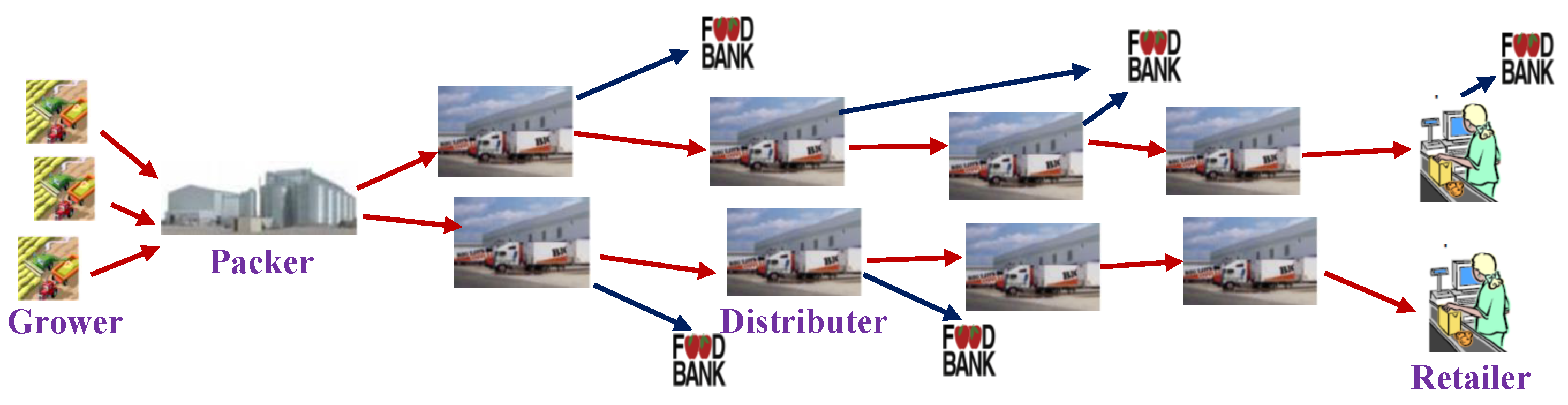
The basic diagram of food logistics is shown in Figure 3. Foods from farmlands are taken to the packing centers where they are sorted and packed for delivery to any of the nearest distribution centers (DCs) and retailers. If the quality of some products deteriorates significantly at any stage of the food supply chain, they are sent to the food banks, where they are consumed at lower cost or for free by the people who need them. By distributing the food products that otherwise would be wasted to the food banks, the food loss in the chain can be significantly reduced. The entire process is fairly complicated, due to the inter-dependencies of several issues, ranging from environmental to social, or from economic to food freshness.
2.1. From Private Logistics to Shared Logistics
In the traditional supply chain, trucks often go empty for a variety of reasons besides lack of sharing. It is reported that in the U.S., the trailers are approximately 60% full in the distribution process. The global transport efficiency was recently estimated to be lower than 10% [1]. The effect is not just merely efficiency related. This results in a greater number of truck runs, which increases the environmental impact, as well as the transportation costs. More truck runs turn the drivers into modern cowboys [1], which results in driver shortages and higher turnover rates. The biggest reason for this inefficiency is that in the traditional supply chain, different vendors use their own private network/trucks for product delivery and do not frequently coordinate with each other. For instance, Walmart and Target use their own food network, as well as their trucks in the delivery process, which reduces the transportation efficiency. Other reasons include: (a) the need to return the truck and product containers back to the source so that they will be available quickly to handle the next shipment and (b) the lack of demand or the unavailability of suitable products or its containers to fill the truck on its backwards journey.
To overcome this, in a shared F, the responsibilities of the distribution companies and the shipping companies are first separated. In F, the trucks are not owned by the distribution companies. Rather, the trucks are owned by some shipping companies (similar to UPS, FedEX, etc.), which take delivery orders from different DCs and deliver them to the corresponding destination DCs. This separation serves two key purposes. First, if the truck journeys are scheduled properly, their space can be shared to deliver the demands of different distribution companies. This reduces the empty miles, improves transportation efficiency, as well as reduces carbon footprint and transportation costs. Reducing empty miles reduces the driving burden of the drivers, as well. Second, in such a model, the containers can be provided by the shipping companies so that in a truck’s journey, the containers move with the truck and are loaded/unloaded with the packages that are to be delivered in between the DCs. In this model, returning the empty containers back to the source is not needed. Such a shared model is promising for improving the overall efficiency of the logistics system; however it brings some new challenges. Scheduling of the truck in this shared model needs to account for several factors such as: (a) transportation efficiency, (b) driver’s away-from-home time, (c) delivery freshness of the food packages and (d) road congestion especially in city areas at peak hours. Some of these objectives are contradictory; for example, as the trucks are shared among the DCs, there is always a tradeoff between capacity utilization and loss of quality of perishable products due to additional delays in waiting for a product to carry and loading/unloading. These distribution decisions are made by consulting with the 3PLoperators to ensure collaborative logistics, instead of private logistics decisions made by the individual companies.
2.2. Modeling the Perishability Metric
Traditional supply chain logistics are researched more towards reducing the transportation cost in the delivery process. In F, one of the important factors is the food freshness, which needs to be integrated with the tradition logistics. Fresh food packages deteriorate in quality over time according to complex biochemical processes that depend on the food type, initial quality, temperature, humidity, vibrations, bacterial level and bruises during storage/transportation. For any certain environmental conditions (temperature, humidity, etc.), the food quality deterioration as a function of time t can be described by a non-decreasing function that is henceforth denoted as . The deterioration of food products is nothing but biochemical reactions; thus, can be modeled as a function of some measurable parameters related to the reaction that determines the quality loss.
We describe a metric for estimating the degradation of a measurable parameter of a food product using its time-temperature indicator. Like any other biochemical reactions, in food products, as well, a certain parameter gets converted to another, say , over time. As the reaction proceeds, the concentration of decreases, whereas that of increases. The concentration loss (of ) or gain (of ) of a particular ingredient at any instance can be described by the following equation:
where C is the concentration of the ingredient, k is the rate of degradation that depends on temperature and other factors and n is the order of reaction that is either zero (zero order) or one (first order) for most of the food products. Food products like fruits or vegetables generally follow zero-order degradation or linear decay, whereas products like meat or fish follow first-order degradation of exponential decay. The quality can be measured by checking the concentration of certain ingredients in the food products. For example, the concentration of vitamin C or sulfur can be the quality indicators for different fruits or vegetables, whereas the concentration of bacterium like mesophiles, psychrotrophs, lactobacilli, enterococci, coliforms, etc., can be the quality indicators for meat products.
The rate of concentration loss or gain k at different temperatures can be modeled using the Arrhenius equation [14] as follows:
where is a constant, is the activation energy and and are the gas constant and absolute temperature, respectively. If a food product goes through multiple phases i = 1, 2, …, m with time at the i-th stage and rate (based on temperature ), then the end concentration of an ingredient is given by:
where is the initial concentration of the ingredient. The parameter k can also be obtained from experimental results at different temperatures. In Equation (3), the ± sign represents the loss or gain of concentration depending on the type of the measurable parameter. For example, the vitamin concentrations of fruits or vegetables decay over time, whereas the bacterial growth on meat products adds up with time. Figure 4a shows the vitamin C degradation of different vegetables over time at 20 C, which shows a linear decay; thus, k’s are the slopes of the graphs. Figure 4b shows the effect of storage temperature on vitamin C degradation on cucumber. The exponential growth of certain bacterium on meat substances is also shown in Figure 4c,d, where ’s are the slopes.
We can scale a perishability function of a food product from the level of concentration of some measurable parameters. It suffices to assume that belongs to the real range [0, 1] where 1 means that the product so far has not suffered any quality loss and 0 means that the product has no value. If we know the storage time and temperature of the chain in different stages, we can estimate the delivery quality of a product using the above approach. In reality, because of different disturbances in the food chain (vibrations, change in temperature or humidity, etc.), the quality deteriorates faster or slower than the theoretical expected rate.
3. Product Distribution and Truck Scheduling
With these, we next formulate our truck scheduling problem with the vision of sharing the truck space to deliver food packages among multiple distribution companies. As mentioned earlier, one of the concerns of traditional logistics is the long driving time of the truck drivers, which makes them
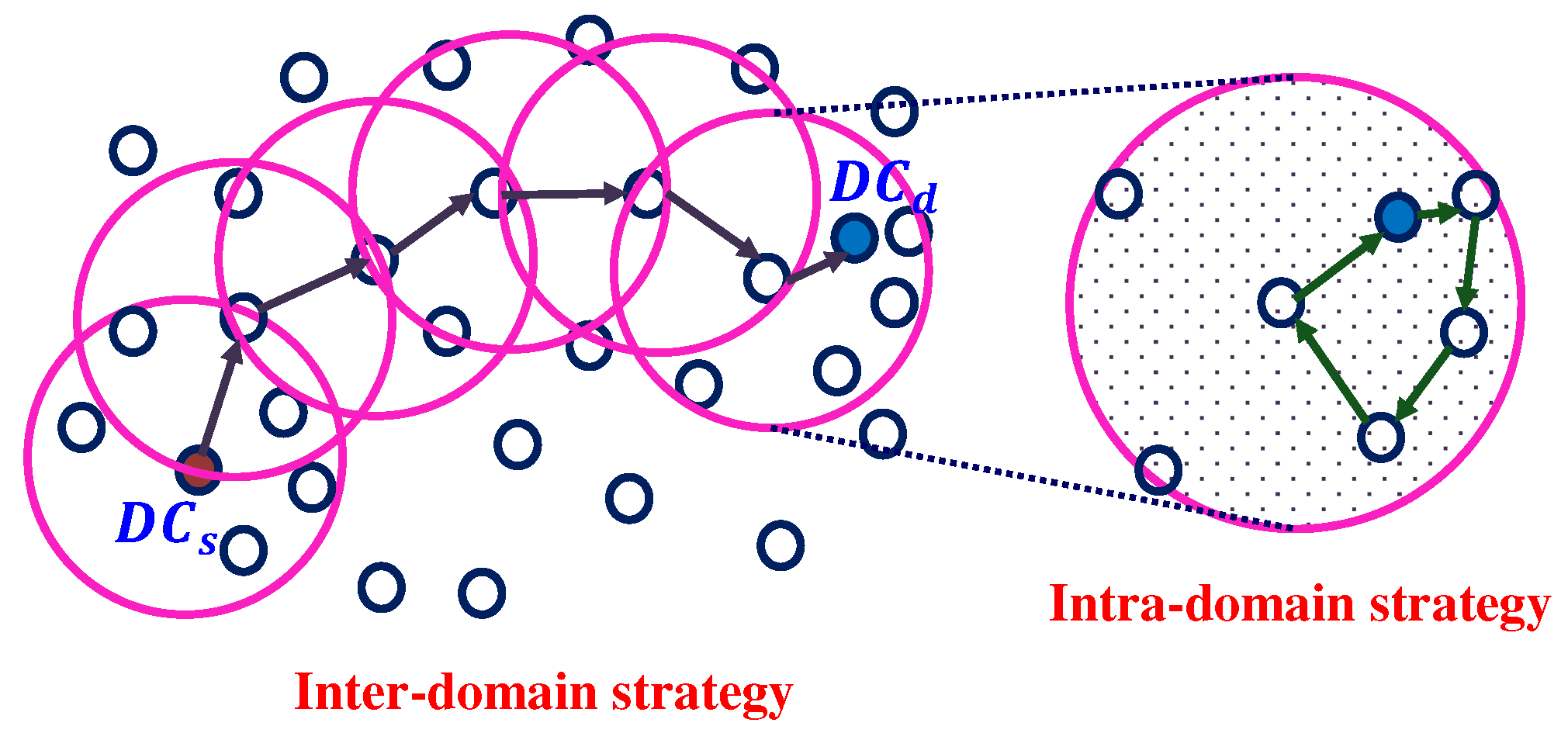
stay away from home for days and sometimes for weeks. To cope with this, in F, the delivery of food packages is done using shorter hops among the distribution facilities. Making shorter trips reduces the driver’s away-from-home time, which improves the quality of his/her personal, social and family life and at the same time reduces his/her turnover rates. An ideal case of this is shown in Figure 5 where the trucks have their certain coverage areas/domains within which they distribute food products among different DCs. The long driving distance in between and is divided into shorter hops, which are determined by inter-domain delivery strategies. When a truck gets an order to deliver something from one DC to multiple other DCs, it checks whether the nearby DCs have to deliver food packages among each other. It then makes its schedule accordingly so that its fuel efficiency or delivery freshness is maximized, and at the same time, the driver can return to the starting point () within his/her scheduled hours. The appropriate scheduling of the trucks within their coverage domains brings the need for developing a smart intra-domain distribution strategy (IntraDS). Proper integration of inter- and intra-domain strategies requires considerations of storage/traveling time of the individual food packages, as well as their delivery requirements, while improving the transportation efficiency of the trucks and their driver-friendly schedules. We discuss the routing and scheduling strategies in these two domains in the following subsections.
3.1. Inter-Domain Strategy
The inter-domain strategy depends on the coverage areas of the trucks. By using the coverage areas of the trucks, as well as the availability of the other transportation modes (rail, river, etc.), the shipping company generates the connectivity graph among the DCs and then implements a routing scheme on this connectivity graph. The routing scheme is similar to the shortest-path routing in computer networks, where the cost function may be a function of a number of factors, like (a) expected delay (waiting time in the DC + travel time), (b) end-to-end delivery quality, (c) the environmental impacts, etc. In F, the shipping companies need to pay extra carbon taxes [19] for using road transportation and prefer river/rail transportation wherever available. Imposing carbon taxes will encourage the shipping companies to use transportation modes that are more environmentally friendly.
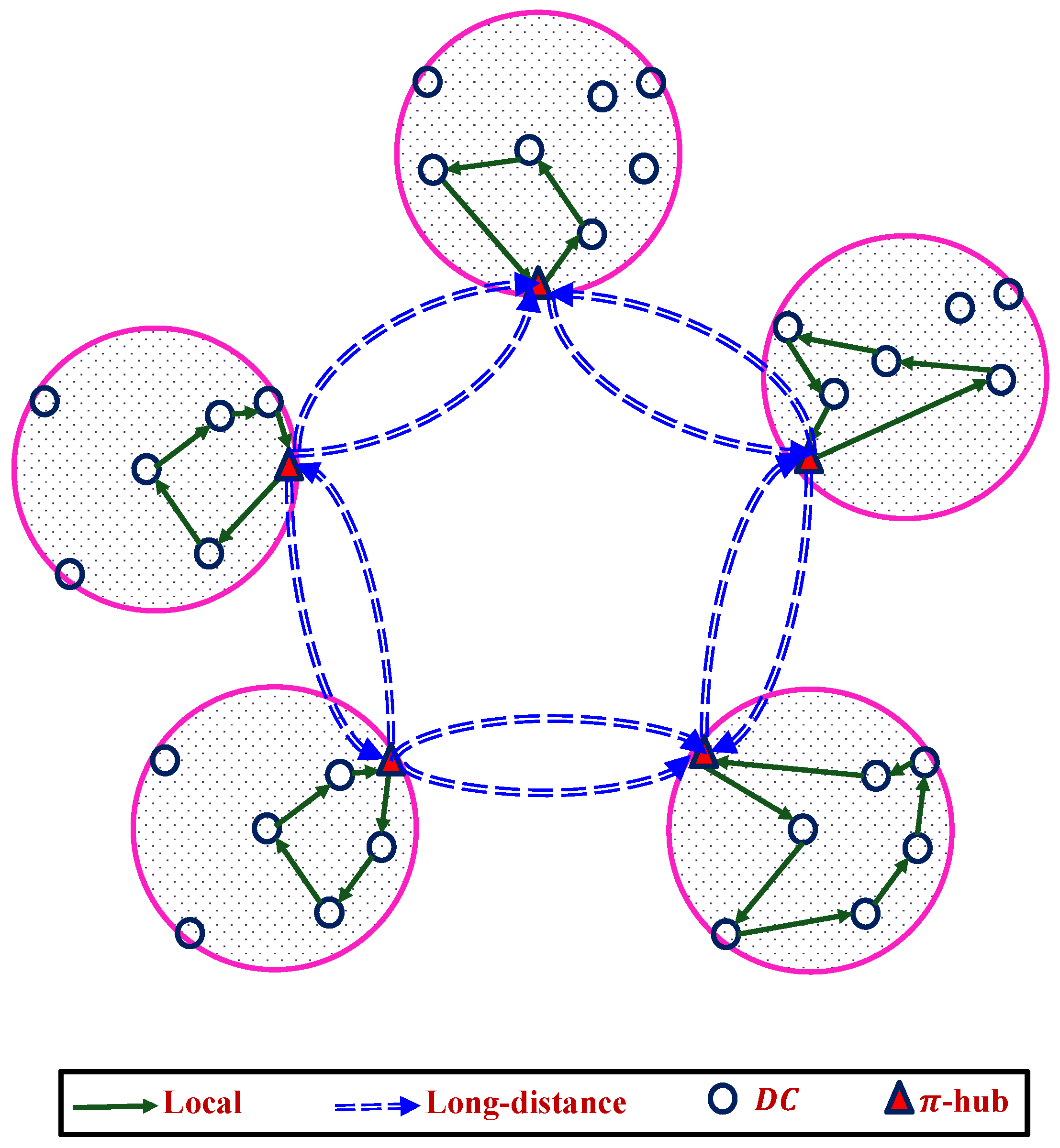
Notice that some of these DCs can be considered as -transit, -switch, -bridge, -gateway, -hub [1], etc., depending on their role in the distribution logistics. For example, Figure 6 shows a scenario that integrates the local and long-distance logistics. In this figure, the local and regional packages are brought at the -hubs for long-distance delivery, which is the distribution of packages in between different regions. The local distribution can be done by small trucks or trailers, whereas the large trucks (18 wheelers) are used for the delivery in between the hubs.
3.2. Intra-Domain Strategy
After getting the delivery orders from the DCs, the shipping companies schedule their trucks for fulfilling the delivery orders, after consulting with the 3PL operators. The truck trips are scheduled in such a way that each driver’s continuous driving time remains limited within which he/she serves as many orders as possible to maximize the design objectives. The Intra-domain routing strategy of the trucks is similar to the traveling salesman problem (TSP) [20], the pickup and delivery problem [21] and the ride-sharing problem [22], but have a number of differences. First, most of the existing schemes are formulated to minimize the overall travel time of the vehicles, whereas our objective is to maximize the fuel-efficiency, reduce the empty-miles and at the same time ensure fresh delivery of the food products to their specified destinations. Second, many of the existing schemes do not put any restrictions on a driver’s (or vehicles) continuous driving time, whereas our scheme needs to ensure that a driver’s away-from-home time is limited, which puts an upper limit on the travel time of the trucks. Third, in the case of the above mentioned problems, a vehicle has to visit every location to serve their requirements, whereas in our scheme, a truck does not need to visit or fulfill the demands of all the DCs within its coverage area. This is because of the fact that the driver’s continuous driving time is bounded. At the same time, visiting few DCs effectively reduces the performance objectives for fewer trucks. Those unfulfilled demands will be delivered by some other trucks. Contrary to the previous works, in our scheme, the truck driver may visit the DCs more than once, which makes the problem even more complicated. Since there may be multiple roads (channels) corresponding to one hop with different periods during a day when they are congested, while scheduling the trucks, the scheduler considers only the road that takes minimum transit time. Notice that the proposed truck scheduling can be applied for distributing packages in both local and long-distance logistics. We next model the optimization problem and then discuss the complexity of IntraDS in the following subsections.
Problem Formulation of IntraDS
The objective of IntraDS is mainly two-fold. First is to maximize the efficiency of the transportation, which we define as the amount of product delivery per miles/time. Second is to maximize the cumulative delivery quality of all the packages, which we define as the product of the delivery quality and the delivery amount. Thus, our objective function is to:
Here, is the initial average quality (for example vitamin C content or other indicators) of the t-th type products from to and k is the quality decay rate at the truck temperature. The term is defined as the efficiency-factor, whereas is defined as the quality-factor. and are the weights of the efficiency-factor and the quality-factor, respectively. Equation (4) assumed linear decay; however, exponential decay can be modeled similar to Equation (3). Notice that the efficiency-factor is basically the package delivery rate of a truck (e.g., the numbers of packages delivered per miles), whereas the quality-factor is a product of the delivery quality and the amount delivered.
The necessary variables for our problem formulation are listed in Table 2. In Table 2, the term transit-segment is defined as follows: if a truck’s travel route is →→→, then the first transit-segment starts at and ends at , the second segment starts at and ends at , and so on. The maximum number of transit-segments allowed for a truck is assumed to be . The source of a truck is denoted as Ⓢ. With these, the constraints of the optimization problem are defined as follows.
Flow conservation constraint: The flow conservation constraint states that, if the truck arrives at any intermediate distribution point j at transit-segment ℓ, then it has to leave from j at transit-segment ℓ + 1, i.e.,
We can also observe that a truck loads and unloads goods at only when it is at the , i.e.,
where is at least as high as the maximum number of objects that can be picked-up/delivered at any particular DC. The number of packages (or goods) that is loaded onto a truck in between any pair of DCs is less than their corresponding delivery requirements. The conservation law also ensures that the cumulative amount of loading and unloading is equal. At the same time, the trucks need to deliver all the loaded packages to their specified destination DCs before the end of their journey. These requirements can be modeled by the following set of constraints:
Truck-load constraint: This constraint states that the truck-load at any transit-segment ℓ is equal to the sum of (a) the truck-load at its previous transit-segment and (b) the difference of the amount that is loaded and unloaded at ℓ. To ensure that a truck is not overloaded, the truck-load at any transit-segment ℓ needs to be lesser than the assigned truck capacity C.
where is the volume of the container type t. Constraint (8) simply assumes that multiple containers of different sizes always fit within a truck as far as their cumulative volume is less than the truck’s capacity. In reality, this is an over-estimation of the packing ability of the containers. In a realistic physical Internet scenario, the packages that are to be transported can be passed to a loading module along with their dimensions, which loads a fraction of the specified packages by solving typical 3D-bin packing [23] with the objective of maximizing the truck space efficiency. The remaining packages wait at the distribution points and are distributed by other trucks while they are scheduled. However, due to the use of modular containers or -containers [1] in the physical Internet, the error due to this over-estimation is limited.
Travel time constraint: To ensure that the drivers do not need to drive continuously for long hours, the total driving time of a truck is limited to . At the same time, to make the scheme realistic and efficient, we want to ensure that whenever a truck starts its journey, it travels for at least time units so that it can travel to multiple DCs and return back to its starting point. Notice that and may vary depending on the type of vehicles (i.e., small trailers or large 18 wheeler trucks), as well as their service types (i.e., whether they are used for local or long-distance logistics, or whether they are operating within a city or between cities, etc.). The total travel time of a truck is bounded by the minimum and maximum allowed driving time, which can be modeled by the following constraints:
The delivery time at the DCs is recorded as follows:
where is assumed to be the time for pickup/delivery at the delivery point j.
Delivery constraint: Other than ensuring space-efficient transportation of the packages, another important feature of F is the delivery freshness. To ensure that the delivered packages maintain a specified freshness limit ℑ, i.e.,
In Equation (11), we assumed the quality decay as linear; however, exponential decay can also be modeled in a similar fashion.
Other constraints: The optimization problem also ensures that the trucks return to their starting points after completing their trips. To keep the problem simple, we assume that a truck does not visit a distribution point more than . For our simulations, we keep as two for simplicity. The above-mentioned constraints can be modeled as follows:
We next define two instances of IntraDS, based on the values of and in Equation (4). When (, ) = (1, 0), the problem becomes an efficiency-factor maximization problem, named E-IntraDS, whereas (, ) = (0, 1) makes it a quality-factor maximization problem, which we call Q-IntraDS.
4. Performance Evaluation
4.1. Performance of Inter-Domain Forwarding
We consider a truck that carries broccoli that has vitamin C content of 99.9 mg/100 g initially. We assume that the broccoli is maintained in two types of environments. One is a chilled environment of 2 C. In the other case, they are carried at 20 C. At 2 C, k = 0.0408 mg/100 g in an hour, where at 20 C, k = 0.1375 mg/100 g in an hour [15,24,25,26].
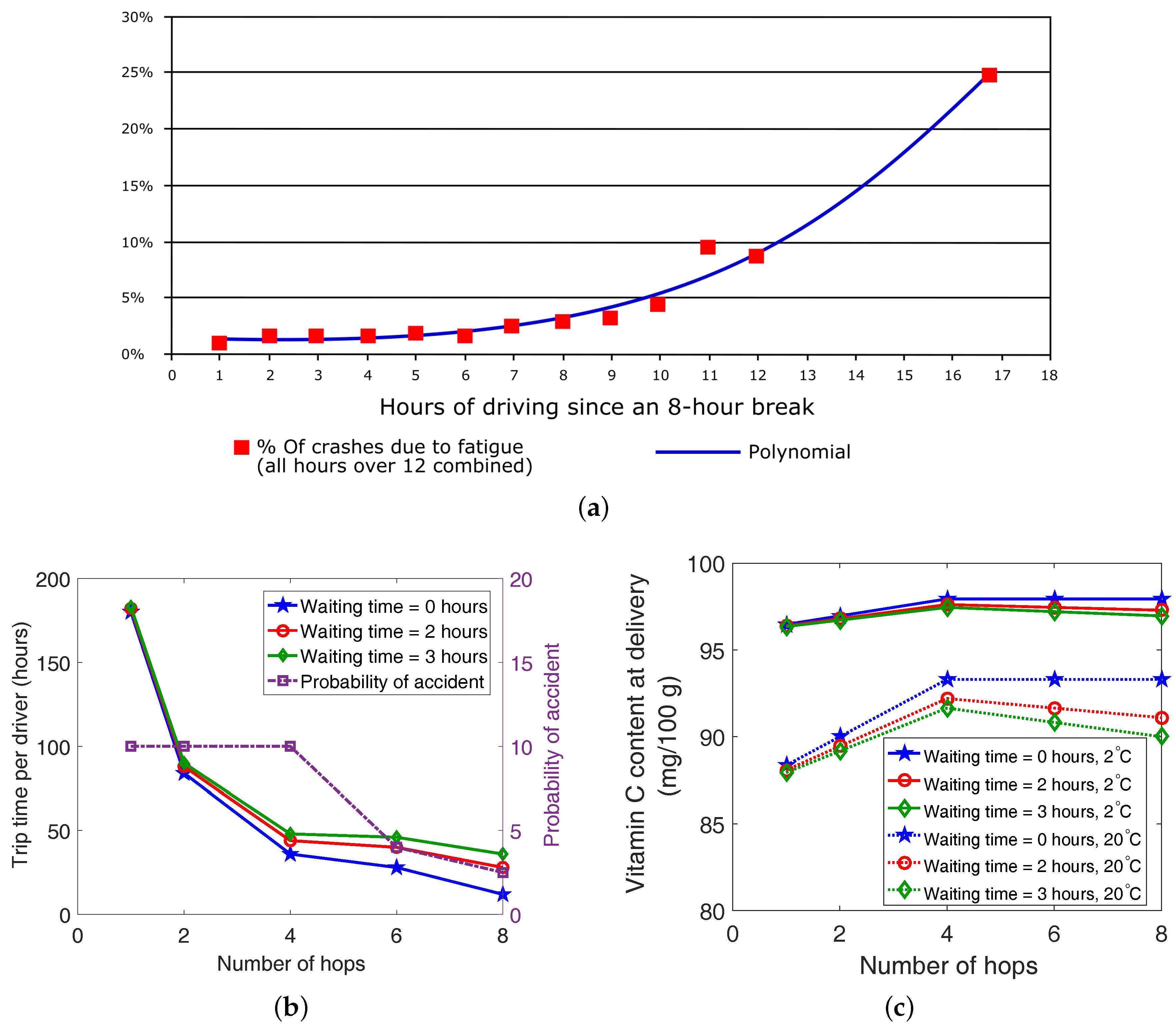
Effect on driver’s driving time: We first demonstrate the advantages of using short hops for delivery among the DCs. We consider a scenario where a truck needs to deliver a certain amount of packages to a DC that requires 48 h of driving time. A driver drives 12 h continuously, takes a rest for 12 h and then starts driving again. The maximum driving time of 12 h is estimated according to the Federal Motor Carrier Safety Administration (FMCSA) regulations [27]; also, the chance of road accidents due to driver fatigue is found to be below 10% within this limit as observed from Figure 7a. If this job needs to be done by a single driver (one hop scenario), then it takes almost 84 h for the driver to reach the destination, deliver the packages, and then, returning back to the starting point takes another 96 h. This long trip time deteriorates the overall quality of the products, as well as increases the driver’s time away from home. In the case of two hops, the driver needs to unload the packages at the halfway point (a DC that is 24 h apart), where another driver loads the packages and delivers them to the ultimate destination DC. This reduces the trip time of each driver as seen in Figure 7. As seen in Figure 7b, by introducing eight hops in between the DCs, the trip time is reduced by ∼93%. Whenever a driver reaches a delivery point, he/she needs to wait for the workers to load/unload the packages to/from the truck, which we vary from 0–3 h in Figure 7. Obviously, the trip time increases due to additional waiting time due to additional loading-unloading.
Reducing the continuous driving time also reduces the chance of driver fatigue and road accidents, as seen in Figure 7a. Thus, using shorter intermediate hops not only reduces the away-from-home time of the truckers, but also reduces the chance of accidents as observed in Figure 7b.
Effect on delivery freshness: The interesting point to note is that increasing the number of intermediate hops improves the delivery freshness. From Figure 7c, we can observe that at 20 C, by introducing eight hops, the vitamin C content in the delivered broccoli is improved by ∼5%, when the waiting time for loading/unloading is assumed to be zero. With the increase in intermediate loading/unloading, the vitamin C content starts decreasing. With eight intermediate hops, the vitamin C content decreases by ∼3% when the loading/unloading time increasing from 0 to 3 h. Figure 7 clearly shows the benefits of using multiple hops for building a worker-friendly fresh food delivery chain. From Figure 7c, we can also observe that the broccoli retains its vitamin contents at a higher level in a chilled atmosphere; the vitamin contents drop by ∼5% if the temperature increases from 2 C to 20 C. Because of additional loading/unloading time in the intermediate points, deciding the number of intermediate delivery hops is an important choice for determining the delivery of fresh quality food, as well as forming a worker-friendly food logistics. Notice that such loading/unloading time and handling of packages during the loading/unloading stage can be largely avoided by the use of modern decoupled truck and trailer units, as discussed in Section 5.2.
4.2. Performance of Intra-Domain Forwarding
We next compare our proposed intra-domain delivery schemes E-IntraDS and Q-IntraDS using a small network that consists of five DCs. The travel time in between the DCs is shown in Table 3, where the DCs are denoted as to . We ignore the pickup/delivery time for simplicity. We use the AMPL solver [29] for solving the optimization problem. We consider two types of packages with raspberries and broccoli. We assume that the containers ensure that the packages are kept at 2 C, which corresponds to the deterioration rates of 0.0229 mg/100 g and 0.0408 mg/100 g per hour, respectively. Their initial vitamin C content is assumed to be 27 and 99.9 mg/100 g. We have normalized these decay rates by assuming the delivery thresholds of raspberries and broccoli to be 25 and 95 mg/100 g, respectively. Thus, their percent deteriorations are 1.15% and 0.83% per hour, respectively. ℑ is assumed to be 0.85. The demand matrix of each one of these two types of food packages among the DCs is shown in Table 4. In Table 4, X is a variable, which is varied from 10–200 for our simulations. We assume all the packages are of the same size of unit volume. The truck has a volume of 100, i.e., its capacity limit is 100 packages, h, and is varied between 6 and 12 h.
Effect on transportation efficiency: Figure 8a compares the efficiency-factor of E-IntraDS with increasing X. From Figure 8a, we can observe that the transportation efficiency starts increasing with the increase in X. This is because with higher X, the truck is loaded with more packages, which increase its efficiency. However, after a certain point, the efficiency saturates. Interestingly, this point is almost similar to all (, ) values, which is X∼ 50 in Figure 8a. Increasing from 6 h–12 h increases the efficiency by ∼80–200%. This is because with higher , the truck gets more time to schedule its route to improve its efficiency, which is limited for lower .
Effect on delivery quality: Figure 8b shows the quality-factor of Q-IntraDS with varying X. The quality-factor increases by 3–5-times with the increase in X from 10–100, as a greater number of packages is transported and delivered. However, after X = 100, this factor starts saturating. Similar to Figure 8a, the saturation point is similar for all (, ) values. We can also observe that the quality-factor increases by four-times, as is increased from 6 h–12 h. This is because with higher , the truck’s travel time increases, as well as the number of loading/unloading operations, which increases the quality-factor.
Figure 8c shows the delivery quality of the packages with different (, ) pairs. We can observe that the delivery quality decreases with the increase in . This is because the higher travel time results in more waiting time of the packages within the truck, which increases their average spoilage. Comparing Figure 8a,c show a clear tradeoff between the transportation efficiency and delivery quality. As we increase the , the efficiency factor increases, whereas the average delivery quality reduces. This is because as increases, the truck delivers more packages to improve its delivery rate, which indeed increases the delivery time and results in quality loss.
Effect on product priority: Figure 8d shows the effect of Q-IntraDS in product mixing. When the demand is low, i.e., X is less compared to the truck capacity, both raspberries and broccoli are carried and delivered; whereas with the increase in X, more broccoli is transported. This is because the percent decay rate of broccoli is much less than that of raspberries, thus delivering more broccoli improves the quality factor, compared to carrying raspberries. We can also observe that the amount of broccoli increases by ∼4-times, when is increased from 6 h–12 h. This is obvious because of the higher number of carried packages with increased travel time.
In Figure 8d, the amount of broccoli delivered is always higher than raspberries, as the spoilage rate of broccoli is lesser. With such an objective function, the products that are more perishable are always given lower preference. To overcome this limitation, the objective function can be modified as . In this objective function, the first factor is identical to the objective function of Q-IntraDS, whereas the second factor gives preference to the products that are close to their spoilage limit. Figure 8e shows the effect of the perishable food transportation with the modified objective function, where is assumed to be 0.5. From Figure 8e, we can observe that the raspberries are given more priority while mixing, due to their higher spoilage rate compared to broccoli.
4.3. Performance Evaluation with a Larger Number of DCs
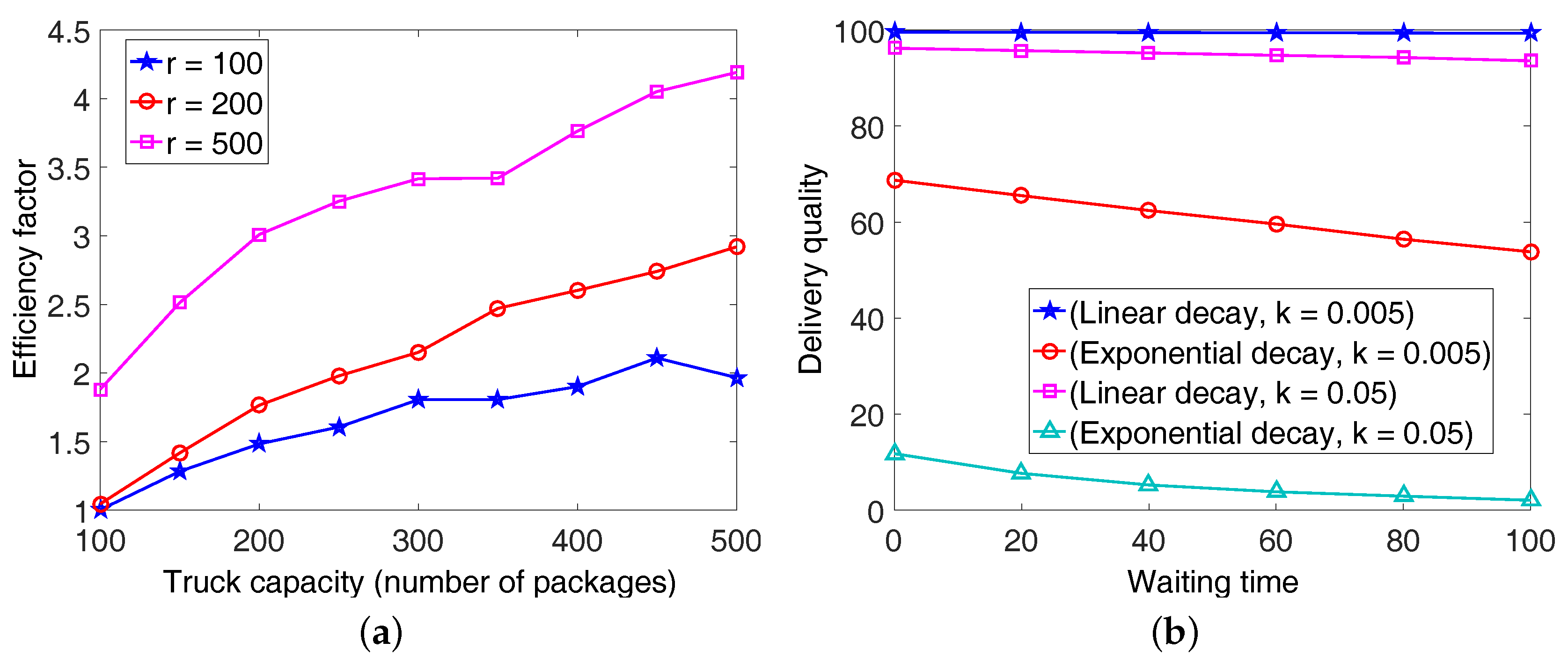
As the proposed intra-domain forwarding is NP-complete, we use a genetic algorithm-based meta-heuristics [30] to evaluate its performance in a large network scenario. For evaluation purposes, we use the MATLAB R2015b [31] simulator where 50 DCs are distributed uniformly in an area of 100 × 100 sq.units. The source-destination DC pairs are generated uniformly and randomly with a probability of 10%. We assume that the source-destination DCs have to ship some packages that are uniformly generated in between (0, r). and are assumed to be of 50 units and 500 units, respectively. We start with one truck for our simulation. If one truck is not sufficient to deliver all the packages, then we gradually increase the number of trucks till all the packages are delivered.
Comparison with different truck sizes: Figure 9a shows the variation of the efficiency factor with different truck sizes. From this figure, we can observe that the transportation efficiency almost doubles when r is increased from 100 to 500. This is because the truck space is better utilized with the arrival of more packages, which improves the transportation efficiency and reduces the empty miles. The efficiency factor also increases by ∼2–3-times while the truck size increases from 100 to 500 as the trucks can deliver more packages during their trips.
Effects of item waiting time on delivery quality: In reality, the packages wait at the distribution points for several hours, before being picked up by the trucks for delivery to their successive destinations. This extra waiting time results in quality loss or spoilage, which we model as a linear and exponential function with spoilage rate k of 0.005 and 0.05 per unit time, respectively. The quality of a fresh package is assumed to be of 100. Figure 9b shows the variation of delivery quality with different package waiting times and spoilage rates. From this figure, we can observe that the waiting time significantly results in quality loss of the packages, especially in the case of the exponential decay model. With k = 0.005 and 0.05, the waiting time of 100 units results in the delivery quality dropping down to ∼50% and <5%, respectively. Such waiting times are unavoidable for large food logistics; however, they can be reduced by ensuring just-in-time supply of packages with respect to the truck arrival at the distribution points.
5. Related Works and Discussions
5.1. Related Works
Modeling of fresh food spoilage has been considered extensively in the literature. A very recent literature work is [32], where the authors have modeled the shelf life of elegant lady peaches using the time-temperature data, over a linear pipeline of four stages: harvesting, warehousing, transportation and retailing. Similar approaches for shelf life modeling are discussed in [33] for chicken breast meat, [34] for ground beef, [35] for mushrooms, etc.
Different planning models for agri-food supply chain, starting from farming, harvesting, storing and distribution, are also well-mined. The work in [36] provides a thorough review of the state of the art in the area of planning models for the different components of agri-food supply chains for both perishable and non-perishable food products. The perishable food literature, which is of primary interest here, is quite recent and often focuses on specific types of produce. Interestingly, as reported in this survey [36], the number of works devoted to production-distribution decisions for the perishable agri-food supply chain is relatively sparse. In [37], an integrated production-distribution plan is developed for the seedling supply chain of a Finish nursery company. The main objective of this model is to minimize the total cost of production and transportation while meeting the customer demands, as well as the capacity-related constraints. The authors in [38] discuss the post-harvest handling of fresh vegetables. The purpose of this research is to maximize the expected profit considering the food preservation facilities, under the conditions of uncertain production and demand. These models typically are optimization models and try to maximize profit or revenue. The work in [39] presents a conceptual model of the supply chain and identifies a number of parameters to quantify the performance of the supply chain network. However, the paper is mostly about defining the metrics and then collecting data for a few case studies. The metrics are classified into four categories that include efficiency, flexibility, responsiveness and food quality. Efficiency metrics relate to things that the network principals care about (e.g., profit, inventory needs, etc.); flexibility metrics are about how easily the network can adapt to a changing environment; responsiveness and food quality mostly deal with customer satisfaction.
Recently, the authors in [4,5,6,7,8] have proposed the idea of imitating the cyber Internet architecture in the physical supply chain to build the framework of integrated and interconnected physical Internet architecture. The authors in [40,41] have introduced a mathematical model for space-efficient packing of a set of products within a requisite number of modular containers. In [42,43,44], the authors have shown that considerable synergies exist between information networks carrying time-sensitive information and perishable commodity distribution networks and have proposed a five-layer network stack to unify the two. Various traceability-related issues for contamination detection in logistics systems are reported in [45,46,47]. To ease traceability for large logistics, the industry has undertaken a produce traceability initiative (PTI), which is already implemented by several large food retailers (including Walmart and Whole Foods) and is being adopted by others (see www.producetraceability.org/). The traceability is ensured by diligently implementing two tasks. The first one is to assign unique IDs (barcodes or RFIDs) to every entity in the network, and the second is to maintain the logs for every individual product that is handled by all the agents. However, these papers have discussed some important points regarding reducing empty or half-empty truck runs, the driver’s long driving time, standardization of modular containers, transportation efficiency, package tracking and traceability, etc., while the food spoilage and quality deterioration of food packages along with several factors that affect the quality loss have not been discussed.
Another related areas is the advancement of several food quality sensors, many of which are currently showing up in the market, such as CSense [48], FoodScan [49], the Salmonella Sensing System [50], etc. These tiny sensors have the ability to sense different quality indicators (such as gas sampling, imaging, etc.) through various forms of contact or non-contact probes. In [51,52], the authors have proposed integrating these quality sensors within the food boxes, to build an online sensing and monitoring framework. As the food boxes carry water-containing products (i.e., fruits and vegetables) or meat packages, the emerging magnetic induction (MI)-based communication is discussed as opposed to typical radio communication, which does not work well in this environment. Such efforts are going to complement our proposed F architecture by making it more robust and quality aware.
5.2. Discussion
The overall proposed scheme is a culmination of several factors that are inspired by the cyber Internet concepts along with the inclusion of physical entities like trucks and drivers. For example, the integration of local and long-distance logistics along with the use of -hubs in Figure 6 is a direct imitation of the hierarchical cyber Internet architecture (i.e., access or regional area networks, metropolitan area networks, core networks, etc.) in the physical space. Intuitively, this results in the package consolidation at the -hubs from different neighboring DCs for long-distance transportation, which results in greater truck load for long-distance large trucks and reduces the long-distance empty miles. In computer networks, time-sensitive packets (like video, audio packets, etc.) are given higher priorities compared to typical data packets, which can also be imitated by tuning the objective function of Problem (4), as done in Figure 8e.
The physical logistics also has certain differences compared to the cyber space: the main difference is the presence of the carriers and their drivers. Redundant carrier transportation results in higher transportation costs, as well as green-house gas emissions. The drivers have their own preferences of shorter driving hours, which is also addressed in this paper. The proposed architecture brings the cyber Internet concepts along with the incorporation of the physical entities (trucks, drivers, etc.) into an integrated optimization framework to improve the overall efficiency, costs, environmental and social impacts of the logistics drivers, which complements the recent physical Internet initiatives.
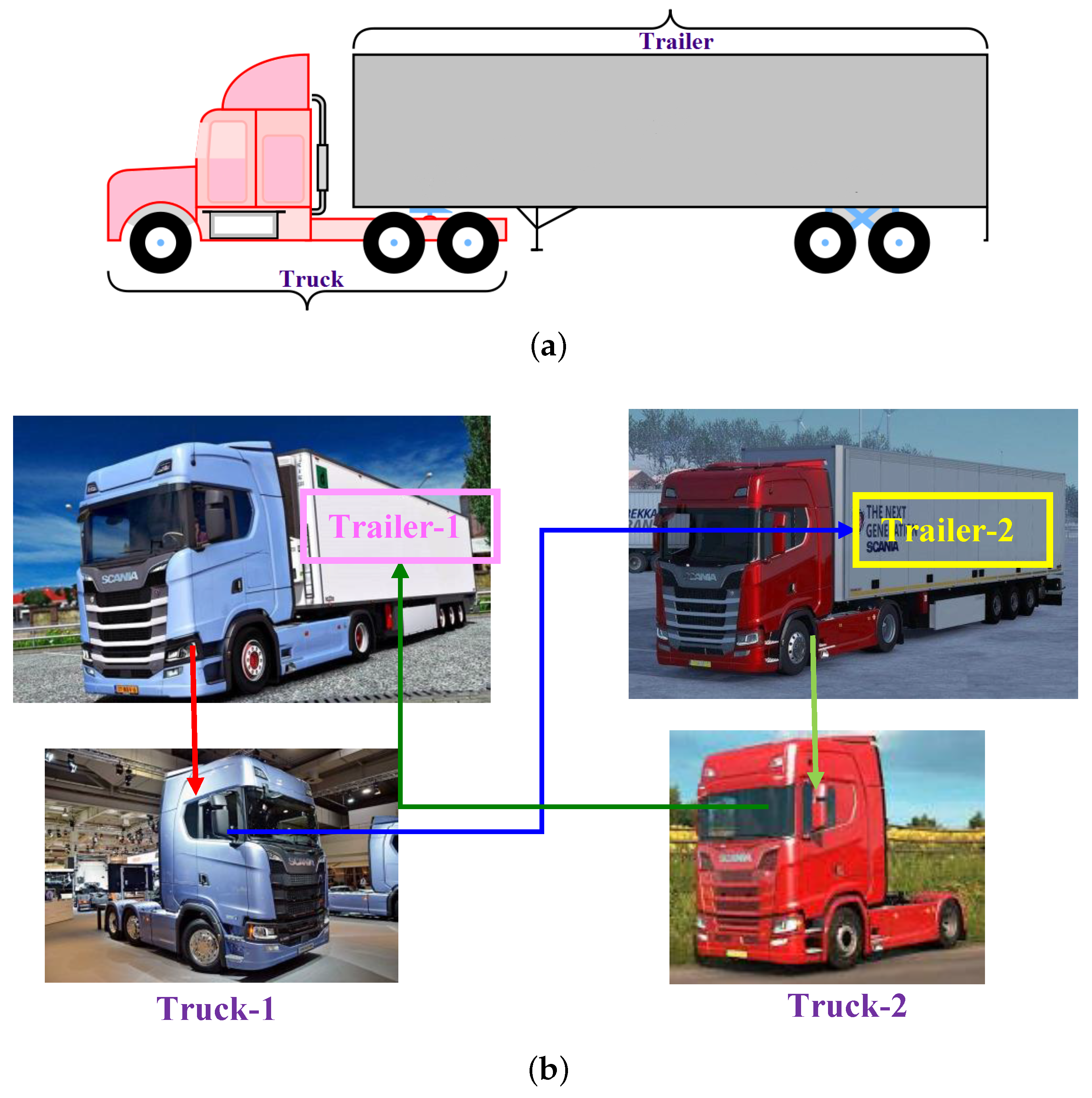
One of the major concerns of the proposed truck scheduling is that many long trips are broken up into smaller short trips. This means that several loading/unloading operations need to be done at the intermediate points. This may be a concern especially in food logistics because these extra loading/unloading operations may deteriorate the product quality. However, such loading/unloading operations are gradually being carried out by automated machinery due to the significant evolution and rapid automation of logistics including robotic processing, loading, unloading, positioning, self-driven vehicles, etc., often referred to as the “Industry 4.0” initiative [53]. Thus, significant care needs to be taken at the intermediate points to ensure that creating extra intermediate hops does not lead to food quality loss. With increasing deployment of decoupled trucks and trailers [54,55], a driver can drive the truck from a point A with a trailer to an intermediate point, exchange his/her trailer with another one (shown in Figure 10) that is destined to A and return back to the starting point. In this way, the loading/unloading operations can be largely avoided; however, there will be some waiting time due to the coupling-decoupling of the trucks and trailers, availability of the trailers that the driver can carry in his/her return trip, etc.
6. Conclusions
In this paper, we introduced the notion of the F architecture and explored the mixing, packaging and delivery of food packages in different parts of the food supply chain. The key characteristics of this proposed architecture are the use of a freshness quality parameter for efficient loading of multiple food products on the trucks and the scheduling of food trucks according to the delivery requirements of individual packages. We further enhanced this architecture with mechanisms to reduce the driver’s away-from-home time while maintaining an end-to-end fresh delivery of the food packages. We believe that the proposed F architecture will complement the existing efforts of emulating the digital Internet in the traditional logistics networks. In the future, we want to include different sensing technologies in F especially for the online monitoring of the food quality and spoilage to make the architecture more robust and efficient.
Acknowledgments
This research was supported by the NSF Grant CNS-1542839.
Author Contributions
The authors worked jointly in the development of the proposed F architecture. A. Pal was involved in the modeling works and data analysis. The paper was written collaboratively by both authors.
Conflicts of Interest
The authors declare no conflict of interest.
References
- Montreuil, B. Towards a Physical Internet: Meeting the Global Logistics Sustainability Grand Challenge. Logist. Res. 2011, 3, 71–87. [Google Scholar] [CrossRef]
- Leuschner, R.; Carter, C.; Goldsby, T.; Rogers, Z. Third-Party Logistics: A Meta-Analytic Review and Investigation of its Impact on Performance. J. Supply Chain Manag. 2014, 50, 21–43. [Google Scholar] [CrossRef]
- GS1 Website. Available online: www.gs1.org/ (accessed on 1 December 2017).
- Montreuil, B.; University, L.; Meller, R.D. Towards a Physical Internet: The Impact on Logistics Facilities and Material Handling Systems Design and Innovation. In Proceedings of the International Material Handling Research Colloquium (IMHRC), Milwaukee, WI, USA, 21–24 June 2010. [Google Scholar]
- Sarraj, R.; Ballot, E.; Pan, S.; Montreuil, B. Analogies between Internet network and logistics service networks: Challenges involved in the interconnection. J. Intell. Manuf. 2014, 25, 1207–1219. [Google Scholar] [CrossRef]
- Pach, C.; Sallez, Y.; Berger, T.; Bonte, T.; Trentesaux, D.; Montreuil, B. Routing Management in Physical Internet Crossdocking Hubs: Study of Grouping Strategies for Truck Loading. In Proceedings of the IFIP International Conference on Advances in Production Management Systems (APMS), Ajaccio, France, 20–24 September 2014; pp. 483–490. [Google Scholar]
- Montreuil, B.; Meller, R.D.; Ballot, E. Physical Internet Foundations. In Service Orientation in Holonic and Multi Agent Manufacturing and Robotics; Springer: Berlin/Heidelberg, Germany, 2013; pp. 151–166. [Google Scholar]
- Ballot, E.; Gobet, O.; Montreuil, B. Physical Internet Enabled Open Hub Network Design for Distributed Networked Operations. In Service Orientation in Holonic and Multi-Agent Manufacturing Control; Springer: Berlin/Heidelberg, Germany, 2012; pp. 279–292. [Google Scholar]
- IPIC2016. Available online: http://www.pi.events/IPIC2016/ (accessed on 10 August 2016).
- Gunders, D. Wasted: How America Is Losing Up to 40 Percent of Its Food from Farm to Fork to Landfill. Natural Resources Defense Council (NRDC). Available online: https://www.nrdc.org/sites/default/files/wasted-food-IP.pdf (accessed on 1 December 2017).
- Pahl, J.; Voß, S. Integrating deterioration and lifetime constraints in production and supply chain planning: A survey. Eur. J. Oper. Res. 2014, 238, 654–674. [Google Scholar] [CrossRef]
- Driver Shortage Report. Available online: https://www.linkedin.com/pulse/driver-shortage-better-pay-plan-dawn-strobel/ (accessed on 1 December 2017).
- Driver Turnover Report. Available online: http://www.conceptservicesltd.com/how-industry-leaders-are-combating-the-truck-driver-shortage/ (accessed on 1 December 2017).
- Laidler, K.J. The development of the Arrhenius equation. J. Chem. Educ. 1984, 61, 494–498. [Google Scholar] [CrossRef]
- Mazurek, A.; Pankiewicz, U. Changes of dehydroascorbic acid content in relation to total content of vitamin C in selected fruits and vegetables. Acta Sci. Pol. Hort. Cultus 2012, 11, 169–177. [Google Scholar]
- Kang, H.M.; Park, K.W.; Saltveit, M.E. Elevated growing temperatures during the day improve the postharvest chilling tolerance of greenhouse-grown cucumber (Cucumis sativus) fruit. Postharvest Biol. Technol. 2002, 24, 49–57. [Google Scholar] [CrossRef]
- Reddy, K.V. Effect of Method of Freezing, Processing and Packaging Variables on Microbiological and Other Quality Characteristics of Beef and Poultry; Retrospective Theses and Dissertations; Iowa State University Digital Repository: Ames, IA, USA, 1981; Available online: http://lib.dr.iastate.edu/rtd/6848/ (accessed on 2 January 2016).
- Quality Aspects Associated with Seafood. Available online: http://www.fao.org/docrep/003/T1768E/T1768E03.htm (accessed on 1 December 2017).
- Benjaafar, S.; Chen, X. On the Effectiveness of Emission Penalties in Decentralized Supply Chains. In Proceedings of the INFORMS Southeast Michigan Symposium, East Lansing, MI, USA, 3 October 2014. [Google Scholar]
- Applegate, D.L.; Bixby, R.E.; Chvatal, V.; Cook, W.J. The Traveling Salesman Problem: A Computational Study (Princeton Series in Applied Mathematics); Princeton University Press: Princeton, NJ, USA, 2007. [Google Scholar]
- Berbeglia, G.; Cordeau, J.F.; Laporte, G. Dynamic pickup and delivery problems. Eur. J. Oper. Res. 2010, 202, 8–15. [Google Scholar] [CrossRef]
- Ma, S.; Zheng, Y.; Wolfson, O. T-Share: A Large-Scale Dynamic Taxi Ridesharing Service. In Proceedings of the 2013 IEEE 29th International Conference on Data Engineering (ICDE), Brisbane, Australia, 8–12 April 2013; pp. 410–421. [Google Scholar]
- Hifi, M.; Kacem, I.; Nègre, S.; Wu, L. A Linear Programming Approach for the Three-Dimensional Bin-Packing Problem. Electron. Notes Discret. Math. 2010, 36, 993–1000. [Google Scholar] [CrossRef]
- Albrecht, J.A.; Schafer, H.W.; Zottola, E.A. Sulfhydryl and Ascorbic Acid Relationships in Selected Vegetables and Fruits. J. Food Sci. 1991, 56, 427–430. [Google Scholar] [CrossRef]
- Albrecht, J.A.; Schafer, H.W.; Zottola, E.A. Relationship of Total Sulfur to Initial and Retained Ascorbic Acid in Selected Cruciferous and Noncruciferous Vegetables. J. Food Sci. 1990, 55, 181–183. [Google Scholar] [CrossRef]
- Lee, S.K.; Kader, A.A. Preharvest and postharvest factors influencing vitamin C content of horticultural crops. Postharvest Biol. Technol. 2000, 20, 207–220. [Google Scholar] [CrossRef]
- FMCSA Report. Available online: https://www.fmcsa.dot.gov/regulations/hours-service/summary-hoursservice-regulations (accessed on 2 January 2016).
- FMCSA Report. Available online: https://www.fmcsa.dot.gov/rules-regulations/topics/hos/regulatoryimpact-analysis.htm (accessed on 2 January 2016).
- Fourer, R.; Gay, D.M.; Kernighan, B. Algorithms and Model Formulations in Mathematical Programming; Springer: New York, NY, USA, 1989; pp. 150–151. [Google Scholar]
- Pal, A.; Kant, K. SmartPorter: A Combined Perishable Food and People Transport Architecture in Smart Urban Areas. In Proceedings of the 2016 IEEE International Conference on Smart Computing (SMARTCOMP), St. Louis, MO, USA, 18–20 May 2016. [Google Scholar]
- Moler, C. Experiments with MATLAB. Available online: https://www.mathworks.com/moler/exm.html (accessed on 2 January 2016).
- Aiello, G.; Scalia, G.L.; Micale, R. Simulation analysis of cold chain performance based on time-temperature data. Prod. Plan. Control 2012, 23, 468–476. [Google Scholar] [CrossRef]
- Park, H.; Kim, Y.; Jung, S.; Kim, H.; Lee, S. Response of microbial time temperature indicator to quality indices of chicken breast meat during storage. Food Sci. Biotechnol. 2013, 22, 1145–1152. [Google Scholar] [CrossRef]
- Kim, Y.A.; Jung, S.W.; Park, H.R.; Chung, K.Y.; Lee, S.J. Application of a Prototype of Microbial Time Temperature Indicator (TTI) to the Prediction of Ground Beef Qualities during Storage. Korean J. Food Sci. Anim. Resour. 2012, 32, 448–457. [Google Scholar] [CrossRef]
- Bobelyn, E.; Hertog, M.L.; Nicolaï, B.M. Applicability of an enzymatic time temperature integrator as a quality indicator for mushrooms in the distribution chain. Postharvest Biol. Technol. 2006, 42, 104–114. [Google Scholar] [CrossRef]
- Ahumada, O.; Villalobos, J.R. Application of planning models in the agri-food supply chain: A review. Eur. J. Oper. Res. 2009, 196, 1–20. [Google Scholar] [CrossRef]
- Rantala, J. Optimizing the supply chain strategy of a multi-unit finish nursery. Silva Fenn. 2004, 38, 203–215. [Google Scholar] [CrossRef]
- Maia, L.O.A.; Lago, R.A.; Qassim, R.Y. Selection of postharvest technology routes by mixed-integer linear programming. Int. J. Prod. Econ. 1997, 49, 85–90. [Google Scholar] [CrossRef]
- Aramyan, L.; Ondersteijn, J.; Kooten, O.; Lansink, A.O. Performance Indicators in Agri-Food Production Chains; Springer: Dordrecht, Netherlands, 2006; Volume 15, pp. 47–64. [Google Scholar]
- Lin, Y.H.; Meller, R.D.; Ellis, K.P.; Thomas, L.M.; Lombardi, B.J. A decomposition-based approach for the selection of standardized modular containers. Int. J. Prod. Res. 2014, 52, 4660–4672. [Google Scholar] [CrossRef]
- Sallez, Y.; Montreuil, B.; Ballot, E. On the Activeness of Physical Internet Containers. In Service Orientation in Holonic and Multi-Agent Manufacturing; Springer: Berlin/Heidelberg, Germany, 2015; pp. 259–269. [Google Scholar]
- Pal, A.; Kant, K. Networking in the Real World: Unified Modeling of Information and Perishable Commodity Distribution Networks. In Proceedings of the IEEE International Physical Internet Conference (IPIC), Atlanta, GA, USA, 29 June–1 July 2016. [Google Scholar]
- Kant, K.; Pal, A. Internet of Perishable Logistics. IEEE Int. Comput. 2017, 21, 22–31. [Google Scholar] [CrossRef]
- Pal, A.; Kant, K. F2π: A Physical Internet Architecture for Fresh Food Distribution Networks. In Proceedings of the IEEE International Physical Internet Conference (IPIC), Atlanta, GA, USA, 29 June–1 July 2016. [Google Scholar]
- Matthews, K.R.; Sapers, G.M.; Gerba, C.P. The Produce Contamination Problem: Causes and Solutions; Academic Press: San Diego, CA, USA, 2014. [Google Scholar]
- GS1 Identification Keys. Available online: http://www.gs1.org/sites/default/files/docs/idkeys/GS1_ID_Keys_Reference_Card.pdf (accessed on 1 December 2017).
- Produce Traceability Initiative Best Practices for Repacking and Commingling. Available online: https://www.producetraceability.org/documents/Repacking_Best_Practice_Guide_v1_2_final_03232012.pdf (accessed on 1 December 2017).
- C2Sense. Available online: http://www.c2sense.com (accessed on 1 December 2017).
- FoodScan. Available online: http://www.israel21c.org/keeping-food-safe-from-farm-to-fork/ (accessed on 1 December 2017).
- Salmonella Sensing System: New Approach to Detecting Food Contamination Enables Real-Time Testing. Available online: http://phys.org/news/2013-10-salmonella-approach-food-contamination-enables.html (accessed on 18 March 2016).
- Pal, A.; Kant, K. Magnetic Induction Based Sensing and Localization for Fresh Food Logistics. In Proceedings of the 2017 IEEE 42nd Conference on Local Computer Networks (LCN), Singapore, 9–12 October 2017. [Google Scholar]
- Pal, A.; Kant, K. Sensing and Communications for Intelligent Fresh Food Distribution Logistics. submitted to ACM HotMobile. 2018. [Google Scholar]
- Hermann, M.; Pentek, T.; Otto, B. Design Principles for Industrie 4.0 Scenarios. In Proceedings of the 2016 49th Hawaii International Conference on System Sciences (HICSS), Koloa, HI, USA, 5–8 January 2016; pp. 3928–3937. [Google Scholar]
- Aurell, J.; Wadman, T. Vehicle Combinations Based on the Modular Concept. NVF-Reports. Available online: http://www.nvfnorden.org/lisalib/getfile.aspx?itemid=1589 (accessed on 2 December 2017).
- Meller, R. Functional Design of Physical Internet Facilities: A Road-based Transit Center; Faculté des Sciences de l’Administration, Université Laval: Quebec City, QC, USA, 2013. [Google Scholar]
Figure 1.
-container architecture [1].
Figure 1.
-container architecture [1].
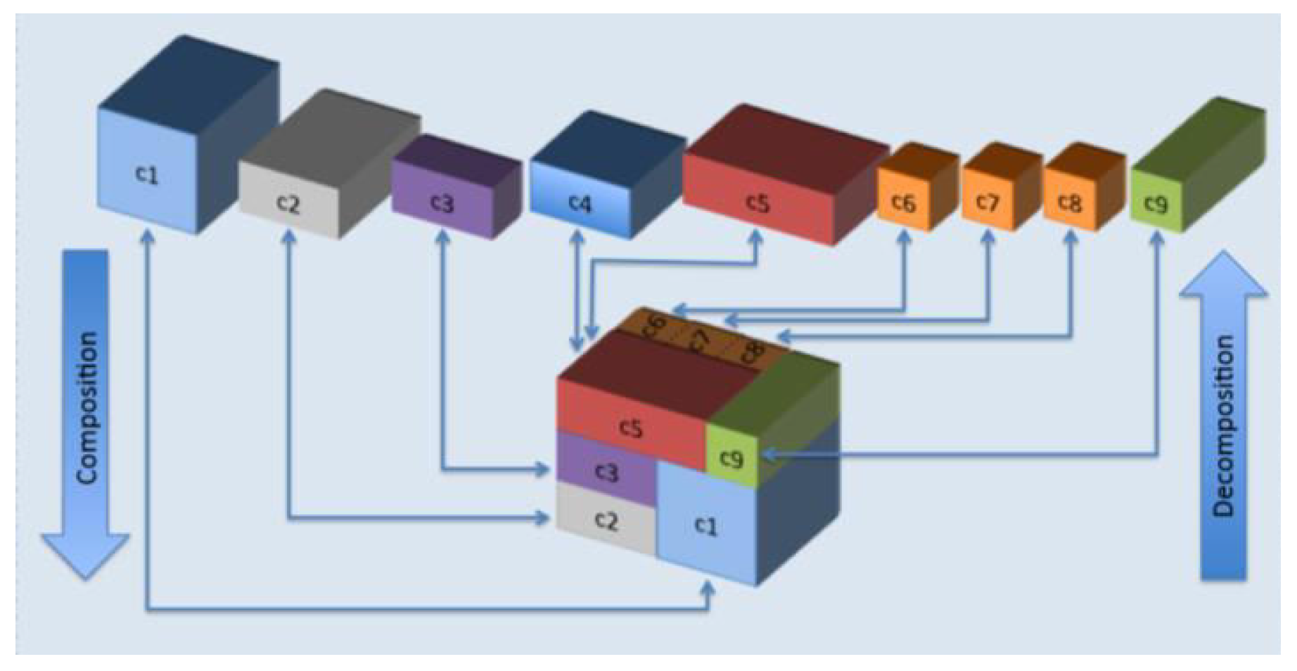
Figure 2.
One key concern of today’s logistics is the long driving and away-from-home time of truck drivers, which results in (a) higher turnover rates [13] and (b) driver shortages [12].
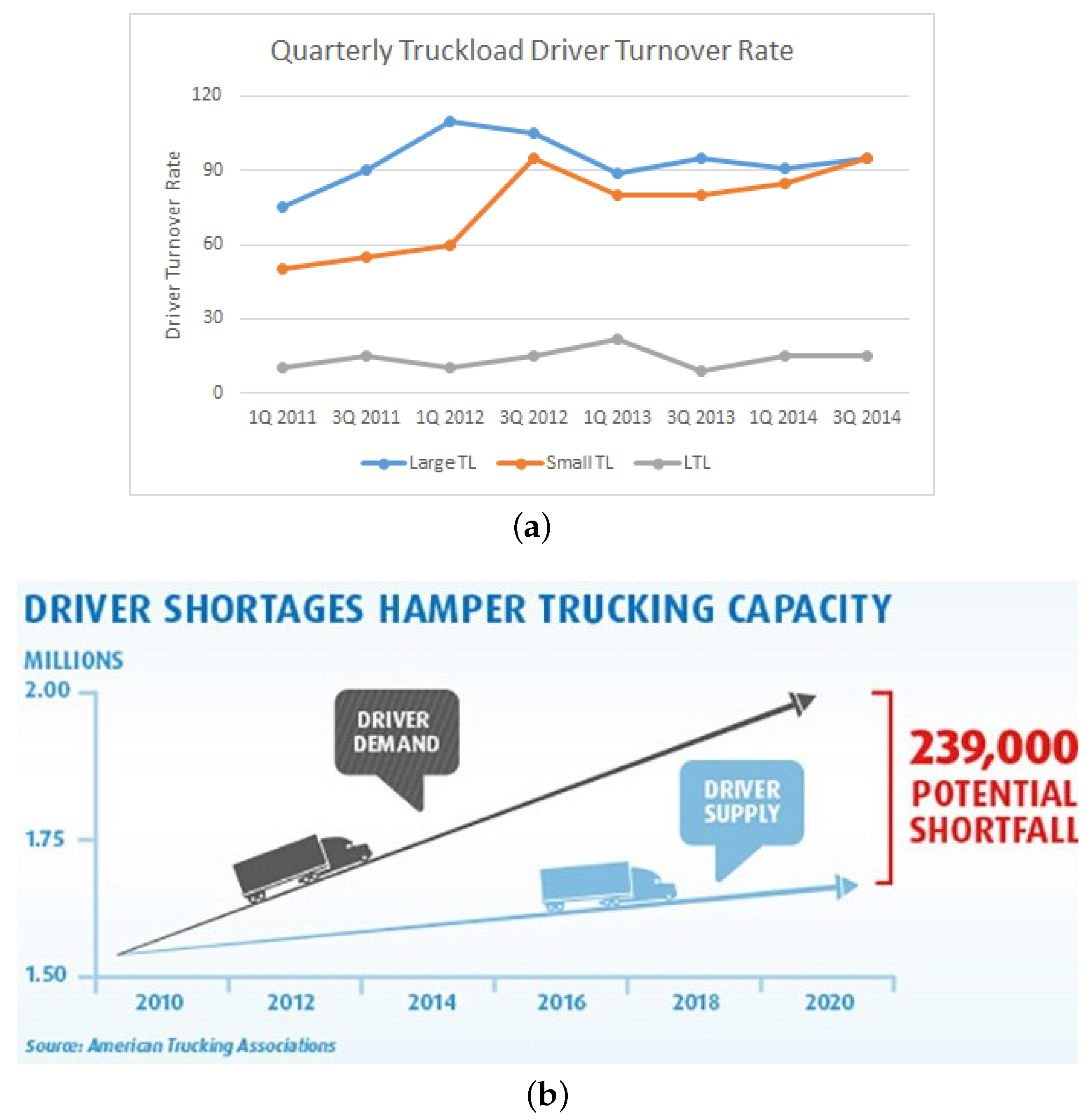
Figure 3.
A schematic of our assumed food network model.

Figure 4.
(a) Vitamin C degradation in different vegetables at 20 C (data obtained from [15]). (b) Changes in vitamin C content of cucumbers grown at control or high temperatures during their storage at 10 or 20 C [16]. (c) Bacterial content in chicken meat at 2 C (data obtained from [17]). (d) Changes in sensory quality of iced cod (0 C) [18].
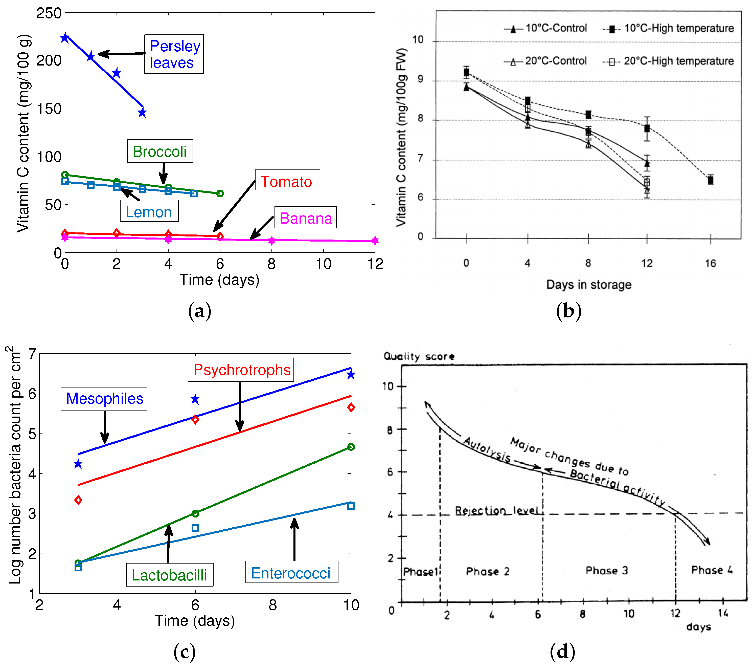
Figure 5.
Inter- and intra-domain schemes between the distribution centers (DCs).

Figure 6.
Integration of local and long-distance food logistics.

Figure 7.
(a) The percentage of accidents due to fatigue as a function of hours of driving [28]. Variation of (b) the trip time of the drivers and (c) vitamin C content at delivery with the number of hops. The waiting time is the time taken at each intermediate hop to load/unload the packages in between different trucks.

Figure 8.
Variation of (a) efficiency-factor, (b) quality-factor, (c) average delivered quality and (d,e) number of delivered packages, with different X. In the legends, and denote raspberries and broccoli, and a and b are and , respectively. Q-IntraDS, quality intra-domain distribution strategy; E-IntraDS, efficiency-factor intra-domain distribution strategy.
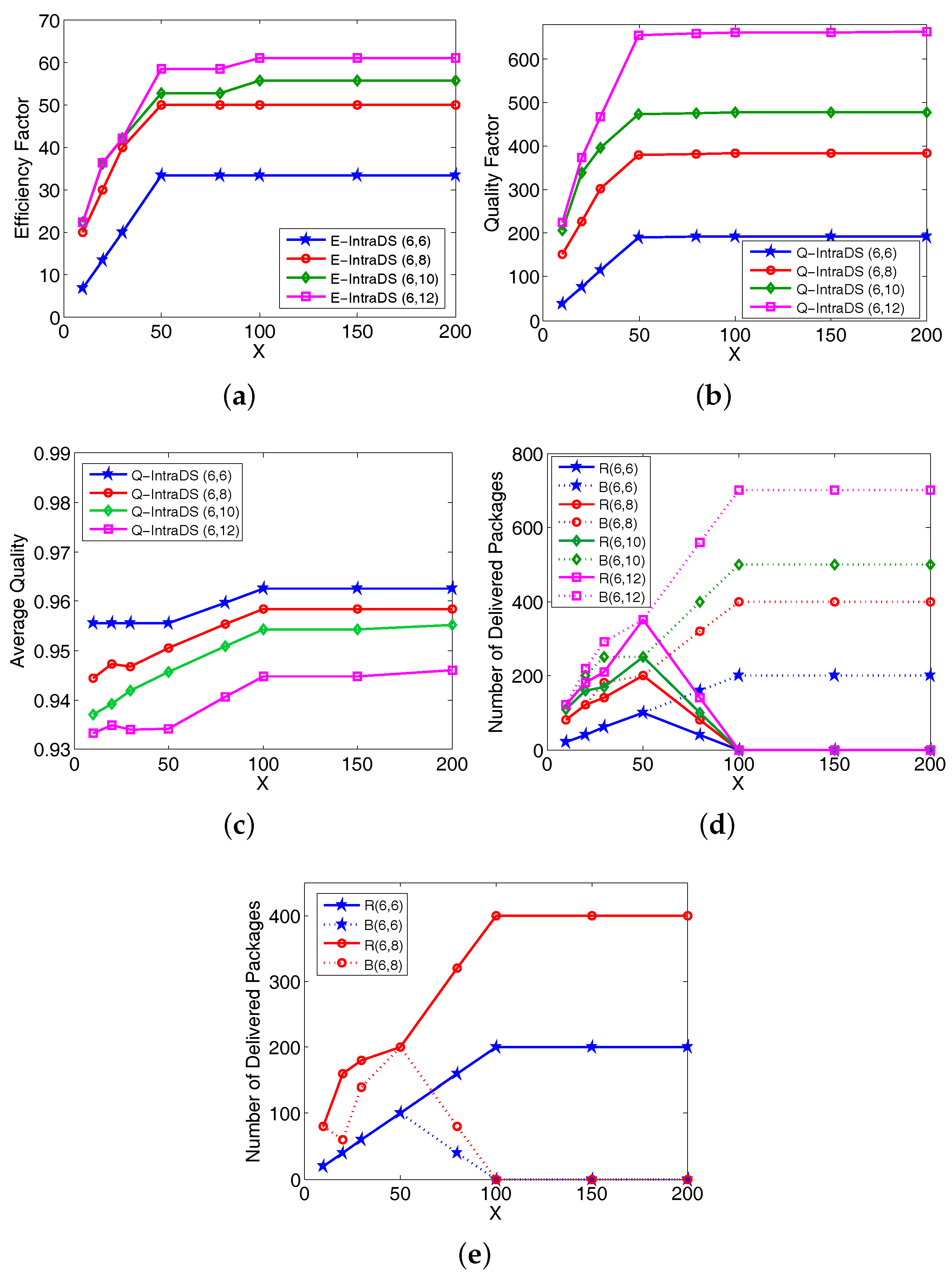
Figure 9.
(a) Variation of efficiency factor with different demand rates. (b) Effect of package waiting time on delivery quality.
Figure 9.
(a) Variation of efficiency factor with different demand rates. (b) Effect of package waiting time on delivery quality.

Figure 10.
(a) Loading/unloading operations at the intermediate exchange points can be greatly reduced by the use of decoupled trucks and trailers. (b) At the transfer points, the trucks (along with the drivers) and the trailers can be decoupled, and Truck 1 can be assigned to Trailer 2 and vice versa. In this way, the loading/unloading operations at the exchange points can be avoided.


Table 1.
Different -nodes and their operations.
| -Nodes | Operations |
|---|---|
| -container | Containers that easily combine to create bigger and bigger containers so as to maximize space utilization and shipping efficiency, as shown in Figure 1 |
| -mover | Moves the -containers, such as -vehicles, -carriers, -conveyors, -handlers, etc. |
| -transit | Exchange points where the -containers are transferred from the inbound -vehicles to the outbound -vehicles |
| -switch | Unimodal transfer of -containers in between the -movers (like rail-rail or conveyor-conveyor -switches) |
| -bridge | One-to-one multi-modal transfer of -containers in between the -movers (like rail-road -bridge) |
| -hub | Multi-modal transfer of -containers from incoming -movers to outgoing -movers, i.e., it transfers the containers in between rail, road, water or air transportation |
| -sorter | Receive -containers from one or more entry points, sort and ship them to their specified exit points |
| -composer | Compose -containers for better space and shipping efficiency |
| -store | Store -containers |
| -gateway | Intersection points in between a private network and the physical Internet |
Table 2.
Table of notations.
| Indices | ||
|---|---|---|
| i, j | ≜ | Index for distribution centers (1, …, ) that are within the coverage areas of the trucks |
| ℓ | ≜ | Index for transit-segments of the trucks (1, …, ) |
| t | ≜ | Index for types of products (1, …, ) |
| Transportation variables | ||
| ≜ | Number of type t loaded at for delivery at at the ℓ-th transit-segment | |
| ≜ | Number of type t unloaded at from at the ℓ-th transit-segment | |
| ≜ | Number of type t that are on the truck for delivery at from at the ℓ-th transit-segment | |
| ≜ | Truck load of type t at transit-segment ℓ | |
| ≜ | Delivery request from to of type t | |
| ≜ | Time of travel from to | |
| ≜ | Time when the truck delivers at in the ℓ-th transit-segment | |
| Decision Variables | ||
| ≜ | Whether or not the truck goes from to at the ℓ-th transit-segment | |
Table 3.
Time matrix.
| A | B | C | D | E | |
|---|---|---|---|---|---|
| A | - | 2 | 3 | 3 | 3 |
| B | 2 | - | 2 | 3 | 3 |
| C | 3 | 2 | - | 1 | 1.5 |
| D | 3 | 3 | 1 | - | 1 |
| E | 3 | 3 | 1.5 | 1 | - |
Table 4.
Order matrix.
| A | B | C | D | E | |
|---|---|---|---|---|---|
| A | - | X | X | X | X |
| B | - | - | X | - | - |
| C | X | - | - | - | X |
| D | X | - | - | - | X |
| E | X | - | X | X | - |
© 2017 by the authors. Licensee MDPI, Basel, Switzerland. This article is an open access article distributed under the terms and conditions of the Creative Commons Attribution (CC BY) license (http://creativecommons.org/licenses/by/4.0/).
Share and Cite
MDPI and ACS Style
Pal, A.; Kant, K. A Food Transportation Framework for an Efficient and Worker-Friendly Fresh Food Physical Internet. Logistics 2017, 1, 10. https://doi.org/10.3390/logistics1020010
AMA Style
Pal A, Kant K. A Food Transportation Framework for an Efficient and Worker-Friendly Fresh Food Physical Internet. Logistics. 2017; 1(2):10. https://doi.org/10.3390/logistics1020010
Chicago/Turabian StylePal, Amitangshu, and Krishna Kant. 2017. "A Food Transportation Framework for an Efficient and Worker-Friendly Fresh Food Physical Internet" Logistics 1, no. 2: 10. https://doi.org/10.3390/logistics1020010