Shaping Light in Backward-Wave Nonlinear Hyperbolic Metamaterials
by
 ,
,
Alexander K. Popov
1,* ,
,
Sergey A. Myslivets
2,3,†,
Vitaly V. Slabko
3,†,
Victor A. Tkachenko
3,† and
Thomas F. George
4,† 
1
Birck Nanotechnology Center, Purdue University, West Lafayette, IN 47907, USA
2
Department of Coherent and Nonlinear Optics, L. V. Kirensky Institute of Physics, Federal Research Center Krasnoyarsk Scientific Center, Siberian Branch of the Russian Academy of Sciences, Krasnoyarsk 660036, Russia
3
Institute of Engineering Physics and Radioelectronics, Siberian Federal University, Krasnoyarsk 660041, Russia
4
Offiice of the Chancellor, University of Missouri-St. Louis, St. Louis, MO 63121, USA
*
Author to whom correspondence should be addressed.
†
All authors contributed equally to this work.
Photonics 2018, 5(2), 8; https://doi.org/10.3390/photonics5020008
Submission received: 25 February 2018
/
Revised: 12 April 2018
/
Accepted: 13 April 2018
/
Published: 18 April 2018
(This article belongs to the Special Issue Nonlinear Dielectric Photonics and Metasurfaces)
Abstract
:Backward electromagnetic waves are extraordinary waves with contra-directed phase velocity and energy flux. Unusual properties of the coherent nonlinear optical coupling of the phase-matched ordinary and backward electromagnetic waves with contra-directed energy fluxes are described that enable greatly-enhanced frequency and propagation direction conversion, parametrical amplification, as well as control of shape of the light pulses. Extraordinary transient processes that emerge in such metamaterials in pulsed regimes are described. The results of the numerical simulation of particular plasmonic metamaterials with hyperbolic dispersion are presented, which prove the possibility to match phases of such coupled guided ordinary and backward electromagnetic waves. Particular properties of the outlined processes in the proposed metamaterial are demonstrated through numerical simulations. Potential applications include ultra-miniature amplifiers, frequency changing reflectors, modulators, pulse shapers, and remotely actuated sensors.
Keywords:
optical metamaterials; fundamental concepts in photonics; light–matter interactions at the subwavelength and nanoscale; fundamental understanding of linear and nonlinear optical processes in novel metamaterials underpinning photonic devices and components; advancing the frontier of nanophotonics with the associated nanoscience and nanotechnology; nanostructures that can serve as building blocks for nano-optical systems; use of nanotechnology in photonics; nonlinear nanophotonics, plasmonics and excitonics; subwavelength components and negative index materials; slowing, store, and processing light pulses; materials for optical sensing, for tunable optical delay lines, for optical buffers, for high extinction optical switches, for novel image processing hardware, and for highly-efficient wavelength converters1. Introduction
The concept of electromagnetic waves (EMWs) with co-directed phase velocity and energy flux is commonly accepted in optics and is true for natural isotropic materials. All optical devices, which we use in everyday life, exploit this concept. However, the advent of the nanotechnology has made possible the creation of metamaterials (MMs) [1] which enable the appearance of the electromagnetic waves with contra-directed energy flux (Poynting vector) and phase velocity (wave vector). They are referred to as backward electromagnetic waves (BEMWs). Such extraordinary properties have opened novel avenues in linear physical optics towards such exceptional (already realized) applications as the subwavelength resolution, clocking of objects, etc. Nonlinear optics (NLO) significantly extends the methods of manipulating light. Most important among them are the possibilities to convert light frequencies. Phase matching of coupled light waves, i.e., equality of their phase velocities, is a paramount requirement for coherent, i.e., phase-dependent, NLO coupling of light waves, which paves a way to efficient frequency conversion and pulse shaping. However, phase matching imposes severe limitations on the choice of practical NLO materials. It has been shown that coherent coupling of normal, forward, EMWs (FEMWs) and BEMWs opens novel avenues for extraordinary NLO processes that hold promise for great benefits in manipulating light. For example, consider parametric amplification at in a transparent material slab of thickness L which originates from NLO three-wave mixing (TWM) and is accompanied by difference-frequency generation of the idler at (). Then, exponential growth of the output amplitudes at and , , inherent to common coupling geometry of co-propagating waves, would dramatically change to for the case of a coupled normal signal wave and contra-propagating BEMW exiting the slab from the entrance edge in the reflection direction [2,3]. Here, the factor g is proportional to the product of nonlinear susceptibility and amplitude of the pump wave at . Furthermore, propagation direction is direction of the energy flux and group velocity. The uncommon “geometrical”, i.e., slab thickness dependent, pump intensity resonance emerges at , which allows for huge enhancements in the NLO coupling, for miniaturization of corresponding photonic devices and for exotic pulse regimes [4]. Four-wave mixing with BEMWs possesses similar extraordinary properties [5,6]. Second harmonic generation (SHG) with BEMWs also experiences significant changes because the fundamental wave depletes and the generated second harmonic (SH) wave grows along the opposite directions [7,8,9]. Therefore, nonlinear energy exchange between the waves at different frequencies traveling with equal co-directed phase velocities, whereas their energy fluxes are contra-directed, offers unusual exciting possibilities in controlling and manipulating light waves. Basically, coherent NLO coupling and quasi-phase-matching of contra-propagating light waves can be achieved in crystals through periodically spatially modulated nonlinearity [10,11,12,13,14,15] where some of the extraordinary processes described below have been or can be realized. The studies are on the way. Discussion of advantages and disadvantages of these approaches is beyond the scope of this paper.
Nonlinear optics deals with phenomena that qualitatively depend on the intensity of the light waves. Hence, qualitative changes occur in NLO processes with BEMs in pulse regimes, because intensities of the coupled fields vary both in space and in time. For example, unusual behavior can be foreseen when the intensity of the pump field varies in the vicinity of the above described “geometrical resonance”. Nonlinear optics with BEMWs holds the promise for the creation of a novel family of photonic devices with extraordinary operational properties and for their significant miniaturization. However, practically the most important is the use of pulsed laser sources of which light intensity varies in time and space. This gives rise to many questions to be answered in the outlined context. Coupling of ordinary and contra-propagating backward pulses is described by a set of coupled partial differential equations. In the case of BEMWs, unusual boundary conditions for amplitudes of the coupled modes must be applied. Numerical solutions of such equations are usually the only approach to the indicated challenging problem. A related research direction of the primary importance is the nanoengineering of the MMs that could support the coexistence of ordinary and BEMWS, which would satisfy the photon energy conservation requirement, travelling with equal co-directed phase velocities while having opposite group velocities. This presents another challenging problem. This paper addresses both outlined challenges of nanoengineering and nonlinear electrodynamics with BEMWs. Theoretical studies and numerical demonstrations are described towards merging nonlinear optics and metamaterials, which pave ways for extraordinary manipulation of light through coherent nonlinear coupling of light waves in deliberately engineered spatially dispersive metamaterials. The possibilities for nanoengineering of a family of novel NLO MMs, which would allow for phase matching of ordinary and backward light waves and for its tailoring to a broad range of frequencies, are demonstrated.
2. Hyperbolic Metamaterials Which Provide Phase Matching of Coupled Guided Contra-Propagating Electromagnetic Waves [16,17,18,19,20,21]
A mainstream in the engineering of the MMs, which can support BEMWs, is grounded on the relationship
This suggests that simultaneously negative electric permittivity and magnetic permeability would result in the direction of the wave-vector to appear against the energy flow (Poynting vector ) at the corresponding frequencies. Such MMs are commonly referred to as negative-index MMs (NIMs). Electromagnetic waves cannot propagate in the materials with , , such as metals. Hence, common major efforts are aimed at the creation of the MMs made of such nanoscopic LC circuits (plasmonic mesoatoms and mesomolecules) that could produce a significant phase delay in the response to the magnetic component of light, which is equivalent to negative . Metallic inclusions provide for negative . Sometimes NIMs are referred to as the left-handed MMs as opposite to the normal right-handed orientation of vectors , and in ordinary materials.
Herewith, we describe a different approach to nonlinear photonics with BEMWs which does NOT rely on optical magnetism. It is grounded on the more general relationship
where is a Poynting vector, U is the energy density, and is the group velocity of light waves. It is seen that the energy flux becomes directed against the wavevector if the directions of the phase and group velocities become opposite. Hence, negative dispersion would give rise to the appearance of BEMW modes [22,23,24]. Equations (1) and (2) are valid for loss-free isotropic materials and used here to demonstrate the distinction between the two approaches. The latter one opens a novel avenue in nanoengineering the MMs that could support both BEMWs and ordinary FEMWs based on different spatial dispersion at different frequencies.
The challenge is to choose such subwavelength building blocks of the MM and to space them in a way that their overall electromagnetic (EM) response would cause such significant phase shift of the propagating EMWs that the normal EM waves convert into backward EMWs (BEMWs). However, the indicated problem is not the sole nor the major one. In the context of the stated goal, most restrictive is the requirement to ensure a set of EMWs at different frequencies satisfying the photon energy conservation law (e.g., ), which are the mixture of normal and BEMWs travelling with one and the same phase velocity (phase matching). Proof-of-principle demonstration of such a possibility and of the flexibility of the proposed approach is presented below [16,19,20,21]. Figure 1 depict a “nanoforest”, the MM made of conducting nanorods of lengths h and of small diameter standing on a conducting surface at a subwavelength spacing and bounded by a dielectric with electric permittivity . The nanoforest is plunged in a dielectric with electric permittivity . The metaslab can be viewed as tampered waveguide. Its eigenmodes and losses depend both on the properties of the constituent materials and shapes of the nanoblocks, as well as on the orientation of the electric and magnetic fields. Numerical demonstrations below refer to a particular case of “carbon nanoforest”, where the MM slab is made of carbon nanotubes (CNTs) of radius r = 0.82 nm spaced at d = 15 nm whereas (air). The choice is motivated by the availability of extensive literature on EM properties of CNTs [25,26,27,28] (and references therein) and by useful THz frequencies of the metaslab’s EM eigenmodes. A carbon nanoforest possesses hyperbolic dispersion because only one component of electric permittivity, , which is along the CNTs, is negative. A review on hyperbolic dispersion properties can be found, e.g., in [29,30,31].
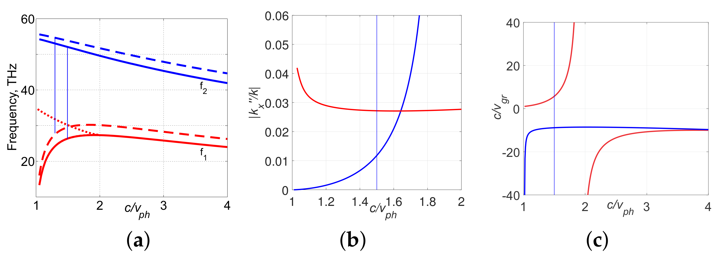
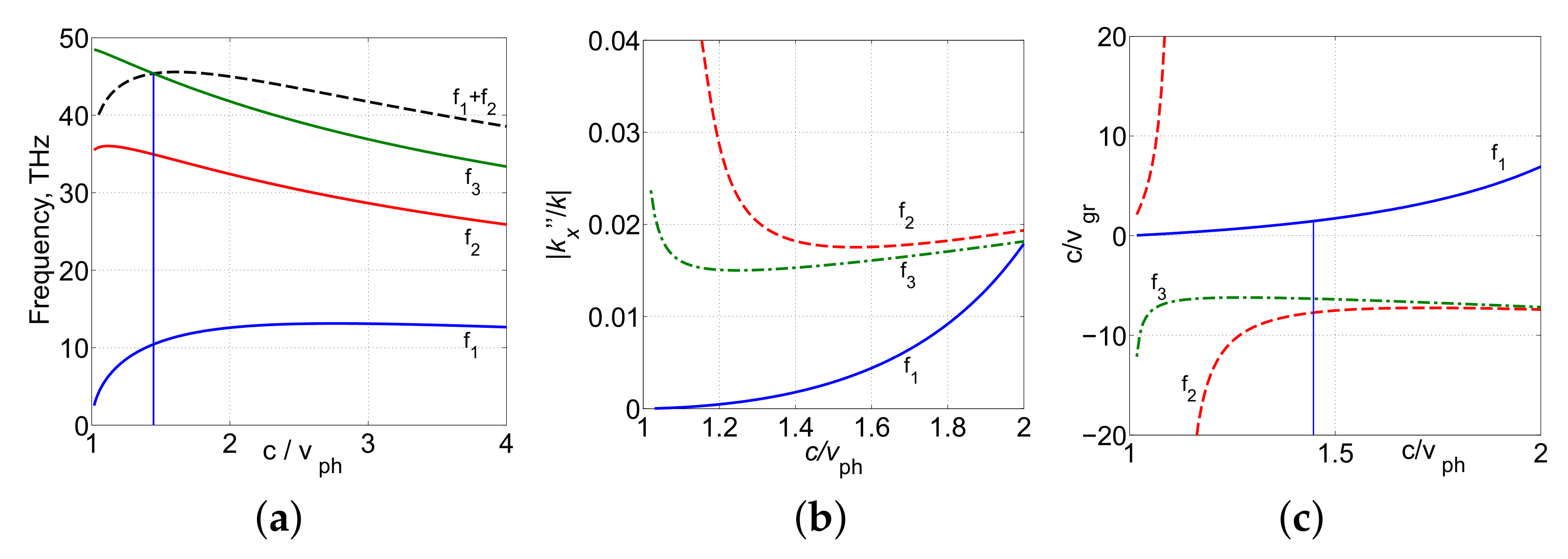
Our studies have shown that the indicated guided eigenmodes peculiar to the given metaslab can be tailored by changing the length of the nanotubes, their spacing, and electrical properties of the bounding and the wafer materials. Most important is that the “nanoforest” can be tailored to achieve phase matching (i.e., equal phase velocities) for the FEMWs and BEMWs, which satisfy the energy conservation law for a given frequency-conversion process over a broad frequency range. Particularly, the example depicted in Figure 2a proves the possibility of phase matching of normal fundamental waves at [] and backward waves at [] for the marked frequencies [19,20] (see also Figure 2c). Figure 3a proves the possibility of phase matching of a normal signal wave at and two contra-propagating BEMWs [] at and (), which can be achieved through adjustment of lengths h of the carbon nanotubes. In the given examples, the matching frequencies fall in the THz and thermal IR frequency ranges. The losses inherent to the coupled guided waves may vary in a broad range and can be tailored as seen in Figure 2b and Figure 3b. Note that group velocities of the matching modes may differ greatly and may include “stopped light” () (Figure 2c and Figure 3c), which paves the way to producing various coupling regimes and to controlling a variety of outcomes.
3. Backward-Wave Second Harmonic Generation [2,7,9,19,20,32]
3.1. Continuous Wave Phase-Matched SHG in a Loss-Free Medium: Forward and Backward Waves
Major differences between the SHG in an ordinary NLO material and in a material that supports BEMWs is explicitly seen in the ultimate case of phase-matched coupling of the continuous fundamental and second-harmonic (SH) waves in a loss-free medium (Figure 4). Figure 4a,b depict a common case of coupling of ordinary, forward waves (FWs). Figure 4c,d depict coupling geometry and photon fluxes corresponding to the fundamental BW and ordinary (forward) SH wave (FSHW).
Figure 4c,d schematically show photon fluxes across the NLO material slab reduced by the input magnitude for the fundamental wave, . are reduced amplitudes of the SH and fundamental waves that are described by the equations
Here, g is the coupling parameter proportional to the SH NLO susceptibility, with the factors for the co-directed fluxes and , for the contra-directed fluxes. The Manley–Rove equation (photon conservation law) derived from Equations (3) is
3.1.1. SHG in Ordinary NLO Medium
For the case of both coupled waves to be FWs (Figure 4a,b), ( and ), one finds from Equation (4) with account for that
This states that sum of the pairs of the fundamental photons and of the generated SH photons is conserved along the medium. The solution to Equations (3) is found as [33]
3.1.2. SHG: Backward Fundamental and Forward SH Waves
In the case of backward fundamental and ordinary SH waves (Figure 4c,d), factors take values and Equations (3) and (4) dictates fundamentally different behavior. Equation (4) predicts
where is a constant, which, however, depends on the slab thickness and on the strength of the input fundamental field. Equations (3) reduce to
Besides the fact that in this case the equations have different signs on the right sides, the boundary conditions for fundamental and SH waves must be applied to opposite edges of the slabs of thickness L: , . Indicated differences give rise to fundamental changes in the solution to the equations for the amplitudes of the coupled waves.
3.1.3. Comparison of SHG for the Cases of Co-Propagating and Contra-Propagating Phase-Matched Waves
Figure 5a illustrates unparalleled properties of SH generation with BWs as compared with its ordinary counterpart at similar other parameters for the particular example of . As noted, the remarkable property in this case is the fact that SH propagates against the fundamental BW and, therefore, metaslab operates as frequency doubling metamirror with reflectivity controlled by the fundamental wave. Figure 5b compares the output intensity of the SH and transmitted fundamental wave for both coupling options. Major important conclusions are as follows. It appears that the efficiency of SHG in ordinary settings exceeds that in the BW, contra-propagating settings at equal to all other parameters. At that, the propagation properties of SH appear fundamentally different, which holds promise for extraordinary applications. The intensity of SH is less than that of the fundamental wave across the BW slab, although it can exceed that in the vicinity of the exit from an ordinary, FW slab (Figure 5a). The quantum conversion grows sharper with an increase of intensity of the fundamental beam, and higher conversion at lower intensities occurs for the co-propagating coupling as compared with that for the counter-propagating coupling.
3.2. Pulsed Regime
In the general case of the pulsed regimes, phase mismatch, different group velocities and lossy medium, SHG is described by the following equations [9]:
Here, the quantities are proportional to the time-dependent photon fluxes ; ; ; ; the coupling parameter ; ; is the effective nonlinear susceptibility; the loss and phase mismatch parameters are and ; ; are are moduli of group velocities and are absorption indices at the corresponding frequencies; is the pump pulse length; is duration of the input fundamental pulse; the normalized slub thickness is and normalized position is ; the normalized time instant . The parameters are for ordinary, and for backward waves.
3.3. Comparison of FW and BW SHG in Short-Pulse Regimes
Significant difference of properties of the SHG pulse regime properties in the FW and BW settings are explicitly seen for the examples considered below, where the input pulse shape is chosen close to a rectangular form:
Here, is the duration of the pulse front and tail, and is the shift of the front relative to . The parameters and have been selected for numerical simulations. Absorption is neglected (). The phase velocities are supposed equal (). The modules of the group velocities are also supposed equal ().
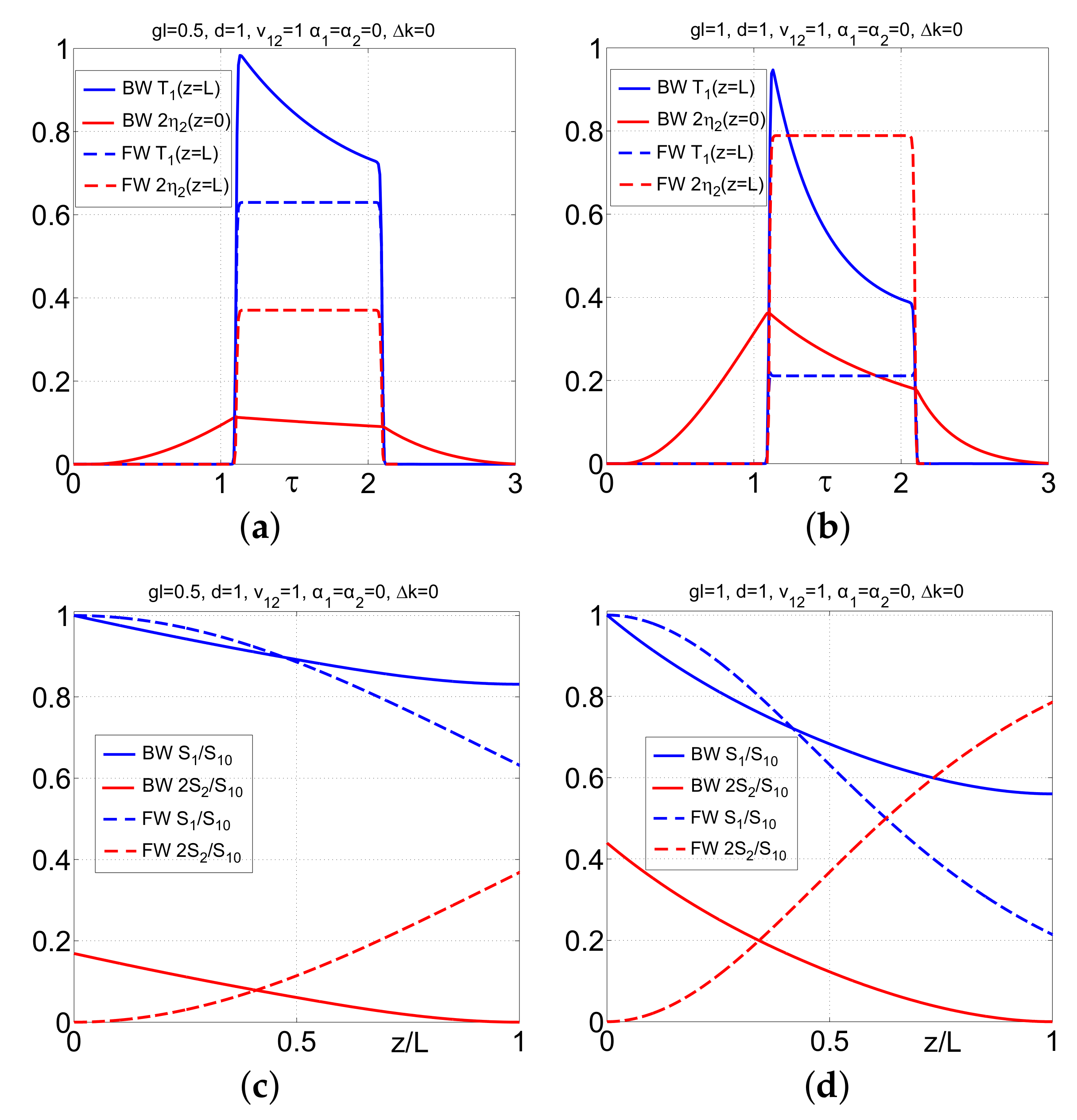
Unusual properties of BWSHG in the pulsed regime stem from the fact that it occurs only inside the traveling pulse of fundamental radiation. Generation begins on its leading edge, grows towards its trailing edge, and then exits the fundamental pulse with no further changes. Since the fundamental pulse propagates across the slab, the duration of the SH pulse may be significantly longer than that of the fundamental one. Depletion of the fundamental radiation along the pulse and the overall conversion efficiency depend not only on the maximum intensity of the input pulse, on the matching of the phase and group velocities of the fundamental and second harmonic, but also on the ratio of the fundamental pulse length and slab thickness. Such properties are in strict contrast with that of FWSHG as illustrated in Figure 6 and Figure 7. The shape of the input fundamental pulse is given by the function when its leading front enters the medium. The results of numerical simulations for the output fundamental pulse, when its tail reaches the slab’s boundary, are given by . The shape of the output pulse of SH, when its tail passes the slab’s edge at , are given by the function . The pulse energies are represented by the time integrated pulse areas that vary across the slab. As seen from Figure 6a,b, saturation is homogeneous across the FWSH pulse, and the shape of both the fundamental and SH output pulses remain rectangular. On the contrary, the shapes of the output fundamental and FWSH pulses are different and change with a change of intensity of the input fundamental pulse. Moreover, it appears that the shapes of the output pulses vary with a change of the input pulse length but at other parameters unchanged, as seen from Figure 7a. The basic properties of the FWSH and BWSH pulse energy conversion across the corresponding slabs qualitatively resemble those in the continuous-wave regime (Figure 6c,d). The unparalleled property of BWSHG is the growth of pulse energy conversion with a shortening of the pulse length with constant instant intensity (cf. Figure 6c and Figure 7b).
Figure 7a,b correspond to the fundamental pulse four times shorter than the slab thickness. They show an increase of the conversion efficiency with an increase of intensity of the input pulse. This is followed by the shortening of the SH pulse.
Figure 6c,d and Figure 7b satisfy the conservation law in a loss-free metaslab: the number of annihilated pair of photons of fundamental radiation ( is equal to the number of output SH photons . Figure 6a,b and Figure 7a prove that shapes and widths of the fundamental and generated SH pulses, as well as the energy conversion efficiency to the reflected pulses at doubled frequency, can be controlled by changing the intensity and ratio of the the input pulse length to the metamaterial thickness (parameter d).
3.4. Backward-Wave Second Harmonic Generation in the Carbon Nanoforest [16,19,20]
For the particular model of the MM depicted in Figure 1a with the nanotubes of height m, the outcomes of the numerical simulation are as shown in Figure 8. The following values and estimates, which are relevant to the MM made of nanotubes of height m, are used for the numerical simulations. The spectrum bandwidth corresponding to the pulse of duration ps is on the order of THz. Hence, , and phase matching can be achieved for the whole frequency band. This becomes impossible at fs because of in this particular case. Phase matching occurs at m, (Figure 2a). Corresponding attenuation factors are calculated as m, m. Since losses for the second mode are greater, the characteristic metaslab thickness corresponding to extinction , i.e., to , , is estimated as m. The pulse length for the first harmonic (FH) is estimated as m, which is 15 times greater than L. The latter indicates that the quasistationary process is established through almost the entire pulse duration, whereas some transients occur at the pulse forefront and tail. Note that, at ps, which is still acceptable, the effect of the transient processes significantly increases.
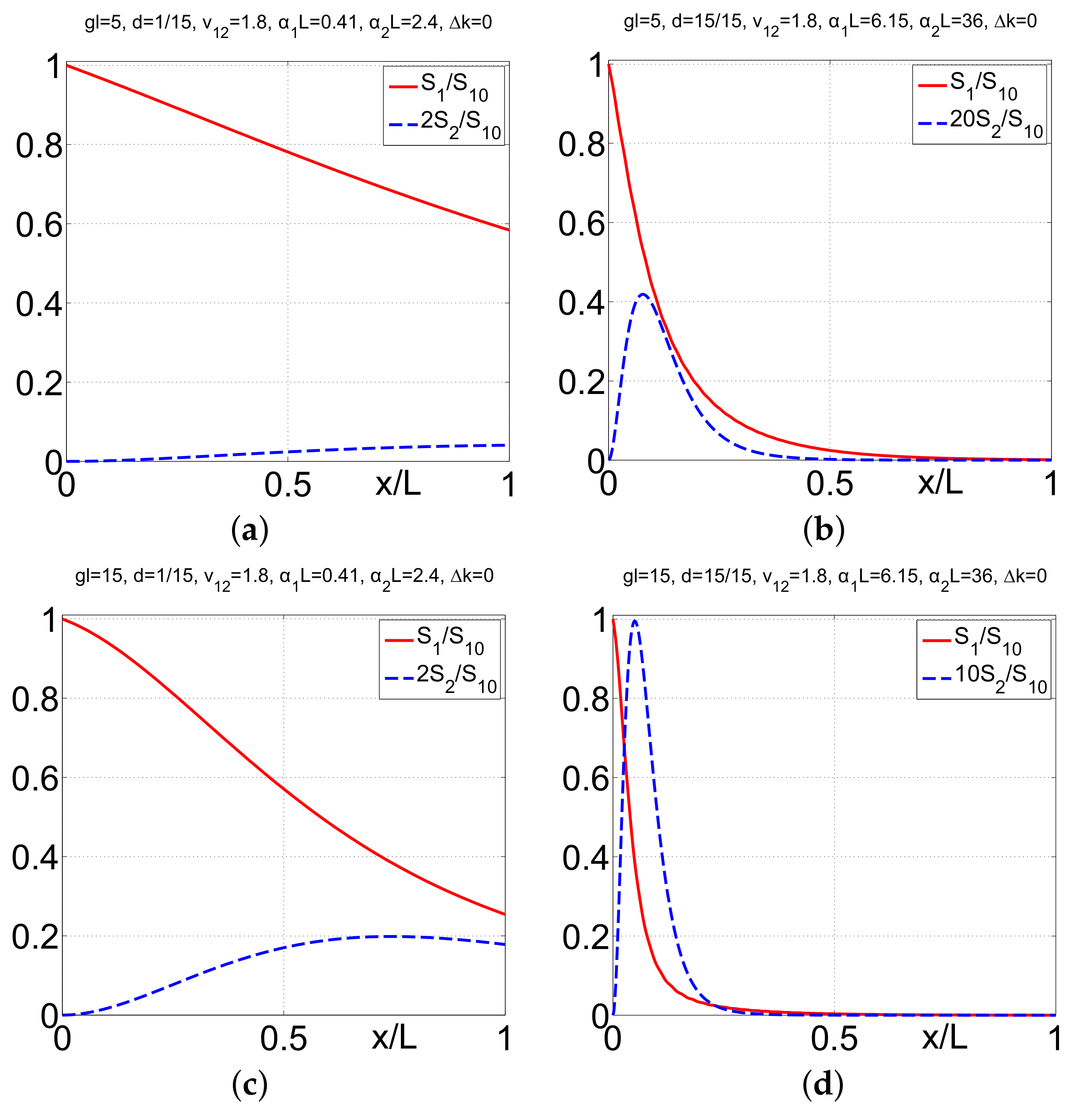
Figure 8 presents the results of numerical simulations for the energy conversion efficiency at BWSHG with an account for the above-calculated losses and group velocities. Here, is the pulse energy (quantum) conversion efficiency, and the factor presents depletion of energy of the FH pulse along the slab and at the corresponding exits: for the SH and for the FH. Two coupling parameters ( and ) and two different input pulse lengths (, and ) are chosen for the simulations. The coupling parameter is proportional to the total number of photons per input FH pulse. It can be also thought of as the ratio of the input pulse length l and the characteristic slab thickness required for the significant photon conversion from FH to SH for the given pulse intensity at its maximum. The interplay of several processes contributes to the outlined dependencies. Figure 8 shows that the conversion efficiency grows with an increase in the input pulse amplitude. However, the important unusual property of BWSHG, i.e., frequency-doubling nonlinear reflectivity, is that it rapidly saturates with an increase of the metaslab thickness. Such unusual behavior is due to the backwardness of SH that propagates against the FH beam and is predominantly generated in the area where both FH and SH are not yet significantly attenuated. It is seen that the overall nonlinear reflectivity provided by such a frequency-doubling meta-reflector can reach values on the order of ten percent for the selected values of the parameter . Calculations also show that the reflectivity in the pulse maximum for the same parameters appears two times greater than the time-integrated values.
These dependencies are in stark contrast with SHG in ordinary materials, as seen from the comparison with Figure 9. These display corresponding dependencies in the case of ordinary materials with all other parameters the same as in Figure 8. Here, both FH and SH exit the slab at . It is seen that, in general, SH reaches its maximum inside the slab. This is due to the interplay of the nonlinear conversion and the attenuation processes. In order to maximize the SH output, the pump strength, its pulse duration, and the slab thickness must be carefully optimized, as shown in Figure 9c. Investigations prove that the shape and the width of the output pulses in the cases of ordinary SHG and BWSHG also appear to be significantly different.
4. Backward-Wave Three Wave Mixing: Parametric Amplification, Nonlinear Frequency-Shifting Reflectivity, Transients and Pulse Shaping [2,3,4,21,34,35]
Three-wave mixing (TWM) with BEMws (BWTWM) also exhibits extraordinary properties. Normalized amplitudes of the waves are given by the following equations, which account for the fact that the propagation direction of the BEMW at must be opposite to others in order to have all phase velocity co-directed and to achieve phase matching (Figure 1b)
Here, , , , , , and are modules of the group velocities and are attenuation indices at the corresponding frequencies, , where , , and is the effective nonlinear susceptibility, . The quantities are proportional to the time-dependent photon fluxes. First, let us consider the ultimate case of continuous waves and neglected depletion of the pump field at .
4.1. Three-Wave Mixing of Continuous Electromagnetic Waves: Approximation of Neglected Depletion of Pump Wave
In this case, equations for amplitudes of the coupled waves reduce to
where . Here, the coupling model is simplified. The equations account for absorption of the incident and reflected coupled fields, whereas depletion of the control field is neglected.
Three fundamental differences in Equations (15) and (16) distinguish them from their counterpart forward-wave three-wave mixing in ordinary materials. First, the signs with g in Equation (15) are opposite to that in Equation (16) because of the backwardness of this wave. Second, the opposite sign appears with because the energy flow is against the x-axis. Third, the boundary conditions for the incident and generated waves must be defined at opposite sides of the sample ( and ) because the energy flows and are counter-directed. Consequently, the equations for and cease to be identical as they are in the case of co-propagating waves in ordinary NLO materials. As will be shown below, this leads to dramatic changes in the solutions to the equations and in the general behavior of the generated waves.
4.1.1. Tailored Transparency, Parametric Amplification and Compensating Optical Losses
If is a BW signal traveling against the pump wave [] and is a difference-frequency generated idler () traveling against the signal [], the slab serves as an optical parametric amplifier at . The transparency/amplification factor is given by the equation
This predicts behavior that is totally different from that in ordinary media. Most explicitly, it is seen at . Then, the equation for transparency reduces to
where , . The equation shows that the output signal experiences an extraordinary enhancement at that can be controlled by adjusting the intensity of the control field (factor g) and/or the slab thickness L. In the given approximation, the equations also show other “geometrical” resonances at , (j= 1, 2, ...). However, they diminish if depletion of the pump field due to amplification of the signal is accounted for. As , parametric amplification turns to parametric oscillations. Such behavior is in drastic contrast with that in an ordinary FWTWM coupling, where in the ultimate case of , the signal would grow exponentially as
The possibility of such extraordinary resonances was predicted for an exotic TWM phase-matching scheme [36] (and in some earlier proposals refereed therein), which has never been realized, and pointed out in a textbook [37]. As suggested in [36], all frequencies were to fall in the positive-index domain, whereas one beam with far infrared wavelength was proposed to be directed opposite to others so that anomalous dispersion could be used for phase matching. However, anomalous dispersion usually occurs in the vicinity of absorption resonances and is accompanied by strong losses. Backward-wave parametric oscillation without a resonator in the radio frequency range was reported in [38]. Coherent NLO coupling of ordinary contra-propagating light waves in the NLO crystals with spatially periodically modulated crystals have been realized in [10,11,12,13,14,15].
4.1.2. Tailored Reflectivity and Nonlinear Optical Metamirror
In the approximation of depletion of the pump being neglected, both coupled weak waves behave in the similar way. Thus, in the opposite case of (the idler with the energy flux against that of the pump wave) and (the signal traveling along the pump wave), the slab serves as an NLO mirror, which emits at against the pump flux . Ultimately, in the approximation of a spatially homogeneous control field and real nonlinear susceptibility, the analytical solution to the Equations (15) and (16) are found, and the reflectivity, , is given by the equation
It is seen that the NLO frequency changing reflectivity also experiences extraordinary enhancement at . For the case of a loss-free slab and exact phase matching, the reflectivity is given by the equation and tends to infinity at , which indicates the possibility of mirrorless parametric self-oscillations. The reflected wave has a differen frequency and, basically, the reflectivity may significantly exceed 100%.
Overall, the simulations show the possibility to tailor and switch the transparency and reflectivity of the metachip over a wide range by changing intensity of the control field. Giant enhancement of the NLO coupling in the vicinity of the geometrical resonance indicates that strong absorption of the BW and of the FW idler can be turned into transparency, amplification and even cavity-free self-oscillations. Self-oscillations would provide for the generation of entangled counter-propagating left-handed, , and right-handed, , photons without a cavity. Energy is taken from the control field. Each point of the slab emits contra-propagating photons, and each of them stimulate emission of the counterpart. Maximum correlation is achieved when the condition is satisfied. Extraordinary enhancement of the NLO (here TWM) coupling occurs due to the outlined distributed NLO feedback, which is equivalent to greatly increasing effective coupling length. It is similar to the situation where a weakly amplifying medium is placed inside a high-quality cavity, which leads to lasing. The outlined features can be employed for the design of ultra-compact optical sensors, selective filters, amplifiers, and oscillators generating beams of counter-propagating entangled photons.
4.2. Three Alternative Coupling Schemes—Three Sensing Options
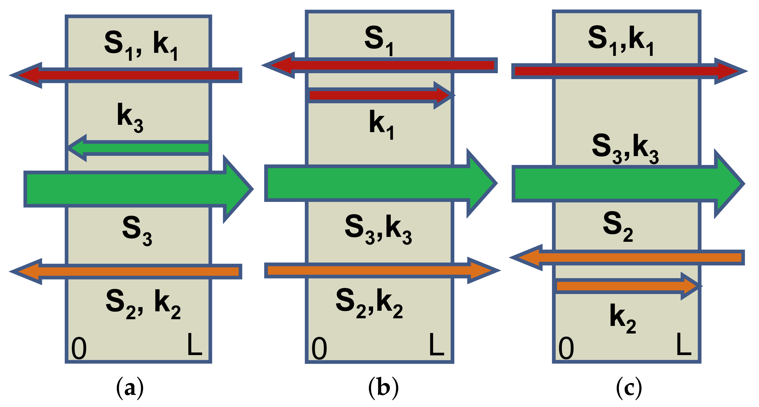
The outlined processes can be applied to all-optical sensing. The corresponding concepts of the prospective sensors are as follows. Figure 10 depicts three possible options for the phase-matched NLO coupling of the ordinary and backward waves.
Consider the example depicted in panel (a). Assume that the wave at with wave-vector directed along the x-axis is an FW signal. Usually, it experiences strong absorption caused by metal inclusions. The medium is supposed to possess a quadratic nonlinearity and is illuminated by the strong higher frequency control field at , which falls into the BW domain. Due to the TWM interaction, the control and the signal fields generate a difference-frequency idler at , which is also assumed to be a FW wave. The idler, in cooperation with the control field, contributes back into the wave at through the same type of TWM interaction, and thus enables optical parametric amplification (OPA) at by converting the energy of the control fields into the signal. In order to ensure effective energy conversion, the induced traveling wave of nonlinear polarization of the medium and the coupled electromagnetic wave at the same frequency must be phase-matched, i.e., must meet the requirement of . Hence, all phase velocities (wave vectors) must be co-directed. Since the control field is a BW, i.e., its energy flow appears directed against the x-axis, and this allows to conveniently remotely interrogate the NLO microchip and to actuate frequency up-conversion and amplification of signal directed towards the remote detector by such a metamirror [39]. The signal can be, e.g., incoming far-infrared thermal radiation emitted by the object of interest, or a signal that carries important spectral information about the chemical composition of the environment. The research challenge is that such a unprecedented NLO coupling scheme leads to changes in the set of coupled nonlinear propagation equations and boundary conditions compared to the standard ones known from the literature. This, in turn, results in dramatic changes in their solutions and in multiparameter dependencies of the operational properties of the proposed sensor. Two other schemes depicted in Figure 10b,c offer different advantages and operational properties for nonlinear optical sensing [34,40].
4.3. Parametric Amplification and Nonlinear Reflectivity in the Vicinity of the Critical Pump Intensity: Extraordinary Transients
As shown, BWTWM experiences extraordinary dependence on the strength of the pump control field. Therefore, extraordinary behavior can be anticipated in the pulse regime, as the pump intensity varies in time. Consider a coupling scheme where the pump at and signal at are co-propagating FWs, whereas the idler at is a BW. Basically, two different regimes are possible. In the first one, the input pump is a semi-infinite rectangular pulse and the input signal is a CW ( = const). In the opposite case, the pump is a CW and is a semi-infinite rectangular pulse. First, consider the case of . The shape of a semi-infinite pulse with a sharp front edge travelling with group velocity v along the axis x is given by the function , where the parameter determines its edge steepness. In the following numerical simulation, it is taken as equal to , where is the travel time of the fundamental pulse front edge through the slab. In the first case, , = const. In the second case, , = const. Here, is a maximum pulse amplitude magnitude at the slab entrance. The solution to Equations (12)–(14) is obtained through numerical simulations.
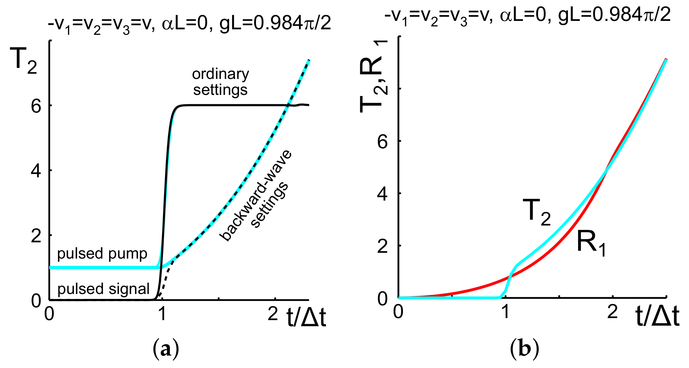
In Figure 11a, the solid line depicts the output signal at the slab exit () for the case of co-propagating ordinary waves, and the dashed line for the case of a BW setting. It is seen that any changes in the output signal occur only after the travel period, both in the ordinary and BW regimes. For the case of a pulsed input pump and CW input signal, the output signal experiences amplification when the forefront of the pump pulse reaches the exit. For the co-propagating settings, the shape of the signal pulse almost follows the shape of the pump pulse. However, in the BW setting, the pulse shape changes dramatically in the vicinity of the resonance intensity of the pump wave, which corresponds to . The signal growth is slower, and the output signal maximum is greater and is reached with significant delay. Figure 11b compares the transmitted signal at and the idler at traveling in the reflection direction for the case of a pulsed input signal and CW pump. This is a travel time of for the signal pulse to appear at , whereas the idler is generated immediately after the pulse enters the slab. Hence, unlike the transmittance, the transients in the reflectivity are the same for the pulsed signal and pulsed pump modes. Figure 11a,b show differences in OPA for the cases of the pulsed signal and pulsed pump disappearing after a period of time about , whereas the reflectivity and OPA develop in a similar way after a period of time about .
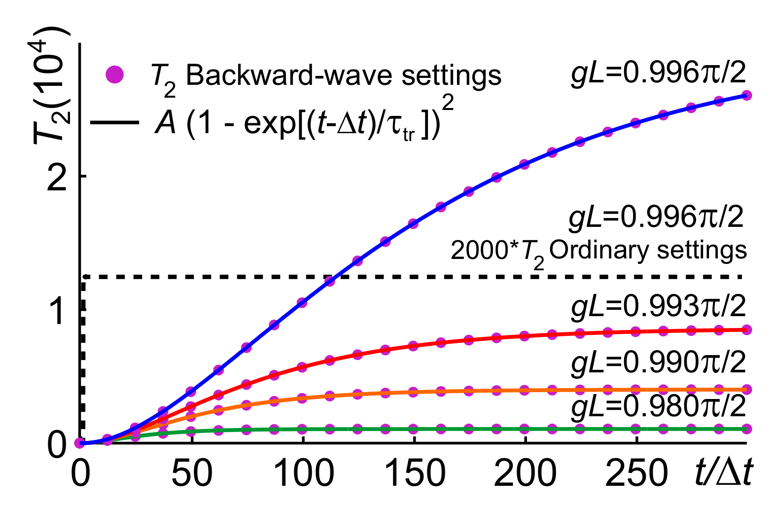
Figure 12 depicts a more extended period of time. It demonstrates that the rise time and the maximum of OPA increase when approaching the resonance strength of the pump field. It also demonstrates the fundamental difference between the rise periods and four orders of difference in the maxima achieved in the ordinary and BW TWM. It appears that calculated data can be approximated by the exponential dependence (solid lines), where the rise time grows approximately as in the vicinity of the intensity resonance. For example, at , the fitting values are , . The short initial period (Figure 11) is not resolved here. As outlined above, the transient processes in OPA and in the NLO reflectivity are similar through the given time period.
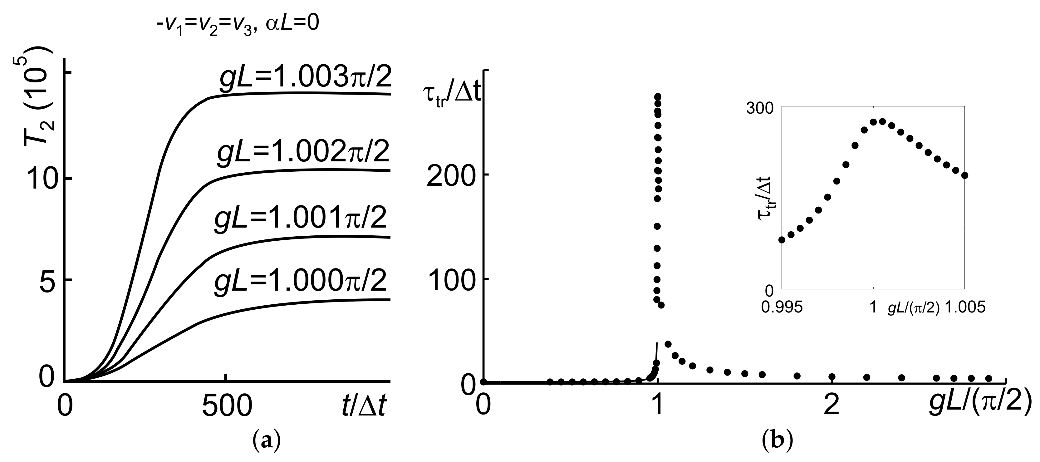
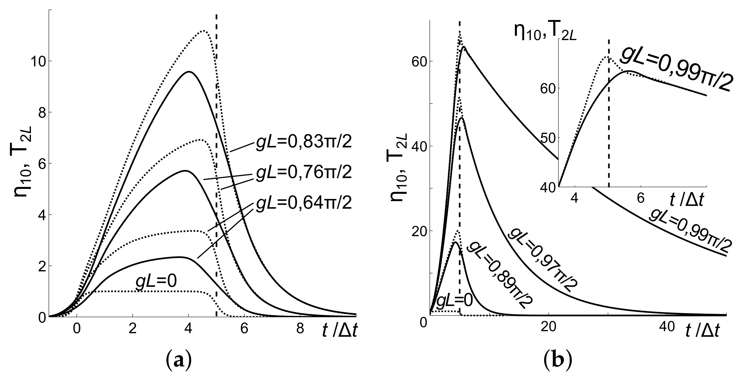
Distributed NLO feedback gives rise to significant enhancement of the OPA and to depletion of the fundamental wave at . The latter leads to the stationary regime and to a decrease of the transient period (Figure 13). As seen from Figure 13b, the delay of the output signal maximum relative to the pump maximum may reach impressive values on the order of hundreds of the travel periods . Maximum delay is reached at .
Absorption causes change in the delay time. For the case of CW and neglected depletion of the pump, the parameter g must be replaced by [2,41]. Hence, losses shift the maximum delay to as seen in Figure 14 and Figure 15a. The described dependencies can be summarized as follows. The opposite direction of phase velocity and energy flux in BEMWs gives rise to extraordinary transient processes, which cause a change in the output pulse shapes and a delay in the formation of their maximums. The closer maximum in the pump intensity approaches the resonance value, the longer becomes the transient period. The delay of the output maximum relative to the input one may occur up to several hundred times longer than the travel time through the metaslab of the forefront of the semi-infinite fundamental pulse. Similar transients emerge in the idler emitted in the opposite direction (in the frequency up- or down-shifted NLO reflectivity). Figure 15b and Figure 16 demonstrate dependence of the transition processes on dispersion of the group velocities.
It appears that changes in the output pulse shapes are strongly dependent on the ratio of the pump and signal pulse lengths, of the pulse lengths and the metaslab thickness, and on the ratio of the pulse group velocities. Figure 17 demonstrates one of the possible scenarios. Here, a continuous wave pump travels through a loss-free slab. Input co-directed FW signal is a rectangular pulse, which is approximately five times longer than the metaslab length L as shown in Figure 17a (for ). Because the BW idler is first generated at the forefront of the signal pulse, their output maximums are shifted. At lower pump intensity, amplification of the rear edge of the signal is greater than the forefront one. As its intensity approaches the critical value , amplification grows, and enhanced idler contributes back to amplification of the signal tail, which leads to significant broadening of the pulses.
4.4. Parametric Amplification and Frequency-Shifting Nonlinear Reflectivity in the Carbon Nanoforest [21]
Consider the particular model of the metaslab depicted in Figure 1b. Figure 3a presents a spectrum of the lowest eigen EM modes and their dispersion calculated for m. For the sake of simplicity, we assume further that . The complex propagation constant is . The reduced wavevector represents the phase velocity . It proves the possibility of the phase-matching for the three-wave mixing frequency down conversion process and OPA at . The simulations also prove the possibility of the phase-matching for different sets of frequencies by adjusting the nanotube lengths h. For convenience, a sum of the mode frequencies is shown by the dashed line. However, only its crossing with the third mode satisfies frequency mixing. Phase matching occurs at (marked with the vertical line). Figure 3c shows group velocity indices for the respective modes. The split for the second mode indicates the slow-light regime . It is seen that in the vicinity of phase matching, the group velocities at and are directed against the phase velocity with the values significantly less than the speed of light. Alternatively, the group velocity for the first mode is of the opposite sign.
Figure 3b depicts attenuation of the respective modes. As seen, the attenuations may differ greatly despite the fact that the electron relaxation rate is the same. The difference is due to the nanowaveguide propagation regime.
At the pump pulse duration ps, the pulse spectrum bandwidth is THz or . Hence, the pump can be treated as quasi-monochromatic. Alternatively, for fs, , the spectrum covers all modes. The data used for the simulations described below are summarized in Table 1. The values indicate the metaslab length corresponding to attenuation , i.e., for the respective frequencies. A thickness m was chosen to satisfy for the mode with highest attenuation. For the same slab thickness, , and . Therefore, attenuation at the lowest frequency appears significantly less than for the two others which are comparable. The pump pulse length for ps is m, i.e., about 6 times greater than . Hence, in this case, a quasi-stationary process is stabilized through the major part of the pulse. Transient processes at the forefront and at the tail of the pulse can be neglected.
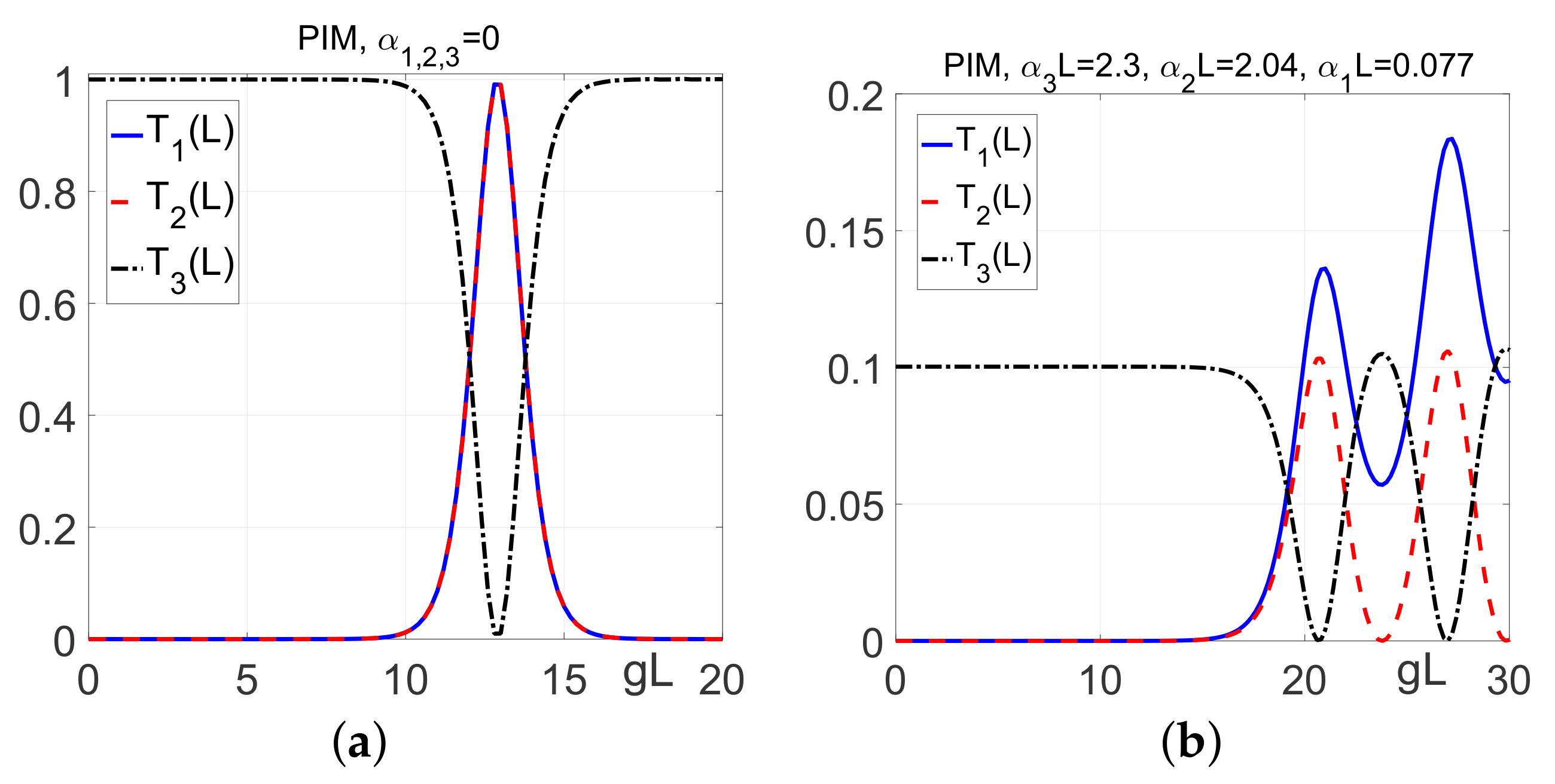
Consider the case where the input signal at is a continuous wave with . Figure 18 demonstrates the dependence of the output amplified signal at and of the idler at generated in the opposite direction on the intensity of the pump, as well as the effects of attenuation and the pump pulse duration on the outputs. Panels (a) and (b) depict the cases of a long pump pulse (quasi-CW regime). Here, are the transmission factors, and is the input pump maximum. The value represents OPA. The nonlinear optical reflectivity (NLOR) at is given by the value . Panel (a), which corresponds to the attenuation-free regime, shows that a huge enhancement in the OPA and the NLOR occurs when the pump intensity reaches a certain threshold value. This is the effect specific to BW coupling, which originates from the appearance of the intensity-resonant distributed NLO coupling feedback addressed above. Here, the photon conversion efficiency reaches 100% at a relatively small increase of the pump above the threshold value. The attenuation significantly decreases OPA (panel (b)). Remarkably, NLOR does not experience such a significant decrease. This is because the reflected wave is predominantly generated near the MM entrance, where the pump and the signal are not yet significantly attenuated. Besides that, the attenuation for the mode appears to be significantly less than the one for the two other modes. Panels (c) and (d) depict the case of a shorter pulse . Here, the transmitted and reflected photon fluxes per pulse are given by the values . It is seen that the dispersion and opposite signs of the group velocities cause a significant increase of the pump threshold and a decrease of the sharpness of the enhancement in the vicinity of the threshold.
The described dependencies are due to the unusual Manley–Rowe relationship. Here, a difference of the pump and of the contra-propagating idler photon numbers is a constant along the slab, whereas the sum of the pump and of the co-propagating signal photon numbers is a constant, as seen in Figure 19 calculated for the ultimate case of the attenuation-free metaslab. The width of the gap between the pump and the idler curves represents a conversion rate. The gap sharply decreases, and the conversion rate increases in the vicinity of the threshold pump intensity.
5. Conclusions
Coherent, i.e., phase-dependent nonlinear optical processes, such as harmonic generation and wave-mixing, play an important role in manipulating light waves by changing frequencies, propagation direction, pulse shapes, and creation of the entangled photons. Properties of such processes experience dramatic changes if some of the coupled waves become backward, while all waves travel with equal phase velocities. Backward electromagnetic waves, also referred to as left-handed waves, are extraordinary waves with contra-directed energy flux and phase velocity (contra-directed group and phase velocities).
Extraordinary properties of the backward-wave second-harmonic generation, optical parametric amplification, and difference frequency generation in the reflection direction are described and contrasted by the comparing with their counterpart in ordinary nonlinear optical materials. Among the unparalleled properties is the appearance of the resonance value of the input pump intensity inherent to backward-wave three-wave mixing, which depends on the nonlinear susceptibility and the thickness of the metaslab. The indicated extraordinary resonance provides giant enhancement in the three-wave coupling. In the vicinity of the resonance intensity, extraordinary transient processes develop, which cause a change in the output pulse shapes and a significant delay in formation of their maximums. The closer the maximum in the pump intensity approaches the resonance value, the longer the transient period becomes. The delay of the output maximum relative to the input one may occur up to several hundred times longer than the travel time through the metaslab of the forefront of the semi-infinite fundamental pulse. Great enhancement occurs both in optical parametric amplification of the signal and in the oppositely directed idler (in the frequency up- or down-shifted reflectivity). Such an effect does not exist in ordinary optical parametric amplification in the case of all co-directed energy fluxes, where the indicated frequency-changing nonlinear reflectivity does not exist either. The described processes hold promise for engineering of a family of miniature photonics devices with unparalleled operational properties. They can also be employed for coherent compensating losses of the backward waves to be used for the numerous extraordinary linear optical applications.
Instead of the commonly accepted concept of the negative-index metamaterials, which can support backward electromagnetic waves, we describe an alternative approach that is grounded on a concept of negative dispersion, . Phase and group velocities become contra-directed if dispersion becomes negative. However, the key requirement in the outlined context is that the metamaterial slab must not only support a set of electromagnetic waves, some of which are backward whereas others are normal, but their frequencies must combine in accordance with the particular process while all waves must travel with the same phase velocity.
We offer a model of the metaslab that can satisfy the set of these requirements as described, which can be employed both for the phase-matched backward-wave second-harmonic generation and backward-wave three-wave mixing. Carbon nanotubes standing on the metal surface, plunged in a dielectric and bounded by a dielectric, are proposed as the building nanoblocks. This (“carbon nanoforest”) possesses hyperbolic dispersion. The corresponding frequencies fall in the THz through near-IR wavelength ranges. The corresponding electromagnetic modes can be viewed as guided modes in a tampered nanowaveguide. We demonstrated that the frequencies, phase and group velocities, as well as the losses inherent to the guided electromagnetic modes supported by the proposed metamaterial, can be tailored to maximize the conversion efficiency and to reverse the propagation direction of the generated entangled photons. This proves that the proposed approach can be generalized for other frequency ranges, and losses can be decreased by changing the constituent materials, size, shape and spacing of the nanoblocks. Among the prospective materials are refractory materials that can work at very high temperatures [42], transparent conducting ceramics [43], and plasmonic materials, where properties can be dynamically tuned [44]. Phase matching of contra-propagating fundamental and backward second harmonic wave in a plasmonic metamaterial is reported in [45]. The described approach can be applied to layered metal-dielectric metamaterials, which include layers of highly nonlinear dielectric as was proposed in [46] for the case of co-propagating waves.
The anticipated properties of the backward-wave second-harmonic generation, parametric amplification, and induced frequency shifting reflectivity are numerically simulated as applied to the particular proposed nanoengineered metaslabs. The described outcomes of numerical simulations of properties of the aforementioned nonlinear optical processes have been presented in the particular proposed backward-wave metamaterials.
Overall, the uncommon behavior of the outlined processes for the proposed advanced metamaterials, both in the time and the space domains, hold promise for the applications to microscopic nanophotonic device technologies, which employ novel principles of extraordinary parametric amplification, switching, and changing the propagation direction and frequencies of the entangled photons.
Acknowledgments
Alexander K. Popov acknowledges support by the U. S. Army Research Office under grant number W911NF-14-1-0619. Vitaly V. Slabko acknowledges support by the Ministry of Education and Science of the Russian Federation (project # 3.6341.2017/6.7).
Conflicts of Interest
The authors declare no conflict of interest. The founding sponsors had no role in the design of the study; in the collection, analyses, or interpretation of data; in the writing of the manuscript, and in the decision to publish the results.
Abbreviations
The following abbreviations are used in this manuscript:
| BW | Backward wave |
| FW | Forward wave |
| MM | Metamaterial |
| FH | First harmonic (fundamental wave) |
| SH | Second harmonic |
| SHG | Second harmonic generation |
| BWSH | Backward wave second harmonic generation |
| TWM | Three-wave mixing |
| BWTWM | Backward-wave three-wave mixing |
| OPA | Optical parametric amplification |
| CW | Continuous wave |
References
- Cai, W.; Shalaev, V. Optical Metamaterials: Fundamentals and Applications; Springer: Berlin/Heidelberg, Germany, 2010. [Google Scholar]
- Popov, A.K.; Shalaev, V.M. Negative-index metamaterials: Second-harmonic generation, Manley Rowe relations and parametric amplification. Appl. Phys. B 2006, 84, 131–137. [Google Scholar] [CrossRef]
- Popov, A.K.; Shalaev, V.M. Compensating losses in negative-index metamaterials by optical parametric amplification. Opt. Lett. 2006, 31, 2169–2171. [Google Scholar] [CrossRef] [PubMed]
- Slabko, V.V.; Popov, A.K.; Tkachenko, V.A.; Myslivets, S.A. Three-wave mixing of ordinary and backward electromagnetic waves: Extraordinary transients in the nonlinear reflectivity and parametric amplification. Opt. Lett. 2016, 41, 3976–3979. [Google Scholar] [CrossRef] [PubMed]
- Popov, A.K.; Myslivets, S.A.; George, T.F.; Shalaev, V.M. Four-wave mixing, quantum control, and compensating losses in doped negative-index photonic metamaterials. Opt. Lett. 2007, 32, 3044–3046. [Google Scholar] [CrossRef] [PubMed]
- Popov, A.K.; George, T.F. Computational studies of tailored negative-index metamaterials and microdevices. In Computational Studies of New Materials II: From Ultrafast Processes and Nanostructures to Optoelectronics, Energy Storage and Nanomedicine; George, T.F., Jelski, D., Letfullin, R.R., Zhang, G., Eds.; World Scientific: Singapore, 2011; pp. 331–378. [Google Scholar]
- Popov, A.K.; Slabko, V.V.; Shalaev, V.M. Second harmonic generation in left-handed metamaterials. Laser Phys. Lett. 2006, 3, 293–296. [Google Scholar] [CrossRef]
- Kudyshev, Z.; Gabitov, I.; Maimistov, A. Effect of phase mismatch on second-harmonic generation in negative-index materials. Phys. Rev. A 2013, 87, 063840. [Google Scholar] [CrossRef]
- Popov, A.K.; Myslivets, S.A. Second harmonic generation and pulse shaping in positively and negatively spatially dispersive nanowaveguides: Comparative analysis. Opt. Quantum Electron. 2016, 48, 143. [Google Scholar] [CrossRef]
- Ding, Y.J.; Khurgin, J.B. Second-harmonic generation based on quasi-phase matching: A novel configuration. Opt. Lett. 1996, 21, 1445–1447. [Google Scholar] [CrossRef] [PubMed]
- Ding, Y.J.; Khurgin, J.B. Backward optical parametric oscillators and amplifiers. IEEE J. Quantum Electron. 1996, 32, 1574–1582. [Google Scholar] [CrossRef]
- Khurgin, J.B. Optical parametric oscillator: Mirrorless magic. Nat. Photonics 2007, 1, 446–447. [Google Scholar] [CrossRef]
- Canalias, C.; Pasiskevicius, V. Mirrorless optical parametric oscillator. Nat. Photonics 2007, 1, 459–462. [Google Scholar] [CrossRef]
- Minor, C.E.; Cudney, R.S. Mirrorless optical parametric oscillation in bulk PPLN and PPLT: A feasibility study. Appl. Phys. B 2017, 123, 38. [Google Scholar] [CrossRef]
- Jang, H.; Viotti, A.L.; Strömqvist, G.; Zukauskas, A.; Canalias, C.; Pasiskevicius, V. Counter-propagating parametric interaction with phonon-polaritons in periodically poled KTiOPO4. Opt. Express 2017, 25, 2677–2686. [Google Scholar] [CrossRef] [PubMed]
- Popov, A.K.; Shalaev, M.I.; Myslivets, S.A.; Slabko, V.V.; Nefedov, I.S. Enhancing coherent nonlinear-optical processes in nonmagnetic backward-wave materials. Appl. Phys. A 2012, 109, 835–840. [Google Scholar] [CrossRef]
- Popov, A.K.; Shalaev, M.I.; Slabko, V.V.; Myslivets, S.A.; Nefedov, I.S. Nonlinear backward-wave photonic metamaterials. Adv. Sci. Technol. 2013, 77, 246–252. [Google Scholar] [CrossRef]
- Popov, A.K.; Slabko, V.V.; Shalaev, M.I.; Nefedov, I.S.; Myslivets, S.A. Nonlinear optics with backward waves: Extraordinary features, materials and applications. Solid State Phenom. 2014, 213, 222–225. [Google Scholar] [CrossRef]
- Popov, A.K.; Nefedov, I.S.; Myslivets, S.A. Phase matched backward-wave second harmonic generation in a hyperbolic carbon nanoforest. arXiv, 2016; arXiv:1602.02497. [Google Scholar]
- Popov, A.K.; Nefedov, I.S.; Myslivets, S.A. Hyperbolic carbon nanoforest for phase matching of ordinary and backward electromagnetic waves: Second harmonic generation. ACS Photonics 2017, 4, 1240–1244. [Google Scholar] [CrossRef]
- Popov, A.K.; Myslivets, S.A. Generation, amplification, frequency conversion, and reversal of propagation of THz photons in nonlinear hyperbolic metamaterial. Opt. Lett. 2017, 42, 4151–4154. [Google Scholar] [CrossRef] [PubMed]
- Agranovich, V.M.; Gartstein, Y.N. Spatial dispersion and negative refraction of light. Phys. Usp. 2006, 49, 1029–1044. [Google Scholar] [CrossRef]
- Agranovich, V.M.; Gartstein, Y.N. Spatial Dispersion, Polaritons, and Negative Refraction. In Physics of Negative Refraction and Negative Index Materials; Krowne, C.M., Zhang, Y., Eds.; Springer Series in Materials Science; Springer: Berlin/Heidelberg, Germany, 2007; Volume 98, pp. 95–132. [Google Scholar]
- Agranovich, V.M.; Shen, Y.R.; Baughman, R.H.; Zakhidov, A.A. Linear and nonlinear wave propagation in negative refraction metamaterials. Phys. Rev. B 2004, 69, 165112. [Google Scholar] [CrossRef]
- Lindell, I.V.; Tretyakov, S.A.; Nikoskinen, K.I.; Ilvonen, S. BW media—Media with negative parameters, capable of supporting backward waves. Microw. Opt. Technol. Lett. 2001, 31, 129–133. [Google Scholar] [CrossRef]
- Nefedov, I.S. Electromagnetic waves propagating in a periodic array of parallel metallic carbon nanotubes. Phys. Rev. B 2010, 82, 155423. [Google Scholar] [CrossRef]
- Nefedov, I.; Tretyakov, S. Effective medium model for two-dimensional periodic arrays of carbon nanotubes. Photonics Nanostruct. Fundam. Appl. 2011, 9, 374–380. [Google Scholar] [CrossRef]
- Nefedov, I.; Tretyakov, S. Ultrabroadband electromagnetically indefinite medium formed by aligned carbon nanotubes. Phys. Rev. B 2011, 84, 113410. [Google Scholar] [CrossRef]
- Argyropoulos, C.; Estakhri, N.M.; Monticone, F.; Alú, A. Negative refraction, gain and nonlinear effects in hyperbolic metamaterials. Opt. Express 2013, 21, 15037–15047. [Google Scholar] [CrossRef] [PubMed]
- Lapine, M.; Shadrivov, I.V.; Kivshar, Y.S. Colloquium. Nonlinear metamaterials. Rev. Mod. Phys. 2014, 86, 1093–1123. [Google Scholar] [CrossRef]
- Poddubny, A.; Iorsh, I.; Belov, P.; Kivshar, Y. Hyperbolic metamaterials. Nat. Photonics 2013, 7, 948–957. [Google Scholar] [CrossRef]
- Popov, A.K.; Myslivets, S.A. Nonlinear-optical frequency-doubling metareflector: pulsed regime. Appl. Phys. A 2016, 122, 39. [Google Scholar] [CrossRef]
- Boyd, R.W. Nonlinear Optics, 3rd ed.; Wiley: New York, NY, USA, 2008. [Google Scholar]
- Popov, A.K. Frequency-tunable nonlinear-optical negative-index metamirror for sensing applications. Proc. SPIE 2011, 8034, 80340L. [Google Scholar] [CrossRef]
- Popov, A.K. Nonlinear Optics with Backward Waves. In Nonlinear, Tunable and Active Metamaterials; Shadrivov, I.V., Lapine, M., Kivshar, Y.S., Eds.; Springer Series in Materials Science; Preface by J. Pendry; Springer International Publishing: Cham, Switzerland, 2014; Volume 200, pp. 193–215. ISBN 3319083856, 9783319083858. [Google Scholar]
- Harris, S.E. Proposed backward wave oscillation in the infrared. Appl. Phys. Lett. 1966, 9, 114–116. [Google Scholar] [CrossRef]
- Yariv, A. Introduction to Optical Electronics, 2nd ed.; Holt, Rinehart & Winston: New York, NY, USA, 1976. [Google Scholar]
- Volyak, K.I.; Gorshkov, A.S. Investigation of backward-wave parametric generator. Radiotech. Electron. 1973, 18, 2075–2082. (In Russian) [Google Scholar]
- Popov, A.K.; Myslivets, S.A. Nonlinear-optical metamirror. Appl. Phys. A 2011, 103, 725–729. [Google Scholar] [CrossRef]
- Popov, A.K.; Myslivets, S.A. Remote sensing with nonlinear negative-index metamaterials. Proc. SPIE 2014, 9157, 91573B. [Google Scholar]
- Popov, A.; Myslivets, S.; Shalaev, V. Resonant nonlinear optics of backward waves in negative-index metamaterials. Appl. Phys. B 2009, 96, 315–323. [Google Scholar] [CrossRef]
- Guler, U.; Boltasseva, A.; Shalaev, V.M. Refractory plasmonics. Science 2014, 344, 263–264. [Google Scholar] [CrossRef] [PubMed]
- Guler, U.; Zemlyanov, D.; Kim, J.; Wang, Z.; Chandrasekar, R.; Meng, X.; Stach, E.; Kildishev, A.V.; Shalaev, V.M.; Boltasseva, A. Plasmonics: Plasmonic titanium nitride nanostructures via nitridation of nanopatterned titanium Dioxide. Adv. Opt. Mater. 2017, 5, 1600717. [Google Scholar] [CrossRef]
- Ferrera, M.; Kinsey, N.; Shaltout, A.; DeVault, C.; Shalaev, V.; Boltasseva, A. Dynamic nanophotonics. J. Opt. Soc. Am. B 2017, 34, 95–103. [Google Scholar] [CrossRef]
- Lan, S.; Kang, L.; Schoen, D.T.; Rodrigues, S.P.; Cui, Y.; Brongersma, M.L.; Cai, W. Backward phase-matching for nonlinear optical generation in negative-index materials. Nat. Mater. 2015, 14, 807–811. [Google Scholar] [CrossRef] [PubMed]
- Sun, Y.; Zheng, Z.; Cheng, J.; Sun, G.; Qiao, G. Highly efficient second harmonic generation in hyperbolic metamaterial slot waveguides with large phase matching tolerance. Opt. Express 2015, 23, 6370–6378. [Google Scholar] [CrossRef] [PubMed]
Figure 1.
An example of the spatially dispersive metamaterial composed of the conducting nanorods of height h. The nanorods stand on the conducting surface and topped by a dielectric layer. The phase-matched energy fluxes at the corresponding frequencies for second harmonic generation (a) and three-wave mixing (b) depicted by arrows. All wave vectors (not shown) are co-directed. Energy fluxes at 2, , and are contra-directed relative their wave vectors due to the negative waveguide dispersion at these frequencies (Figure 2 and Figure 3). Negative wave guide dispersion can be thought as negative refraction at the corresponding frequencies.
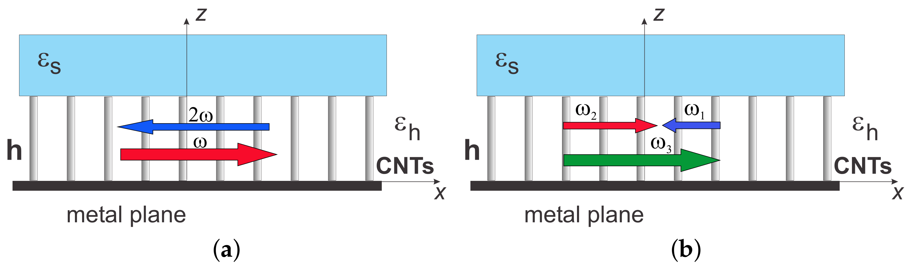
Figure 2.
(a) Dispersion of two lowest eigenmodes in the slabs of standing carbon nanotubes with open ends. ; m (solid lines) and m (dashed lines); (b) attenuation factor for the lower-frequency mode (the descending red plot) and for the higher-frequency second mode (the ascending blue plot) at m; (c) group velocity vs. phase velocity for the same two modes. The descending dotted red line in panel (a) shows one of the very lossy guided modes. The vertical lines in all panels mark the waves travelling with equal phase velocities while satisfying the relation .

Figure 3.
(a) Dispersion of the three lowest modes at m, where , k is wavevector in vacuum for the corresponding frequency f, and is the phase velocity. The vertical line marks the waves travelling with the same phase velocity while satisfying the requirement . The dashed line represents the sum of the two lowest modes; (b) normalized attenuation constant : the blue (solid) line corresponds to , the red (dashed) to , and the green (dash-dotted) to ; (c) group velocity indices for the respective modes.

Figure 4.
Coupling geometry and energy fluxes in ordinary materials (a,b) and in backward-wave materials (c,d).
Figure 4.
Coupling geometry and energy fluxes in ordinary materials (a,b) and in backward-wave materials (c,d).
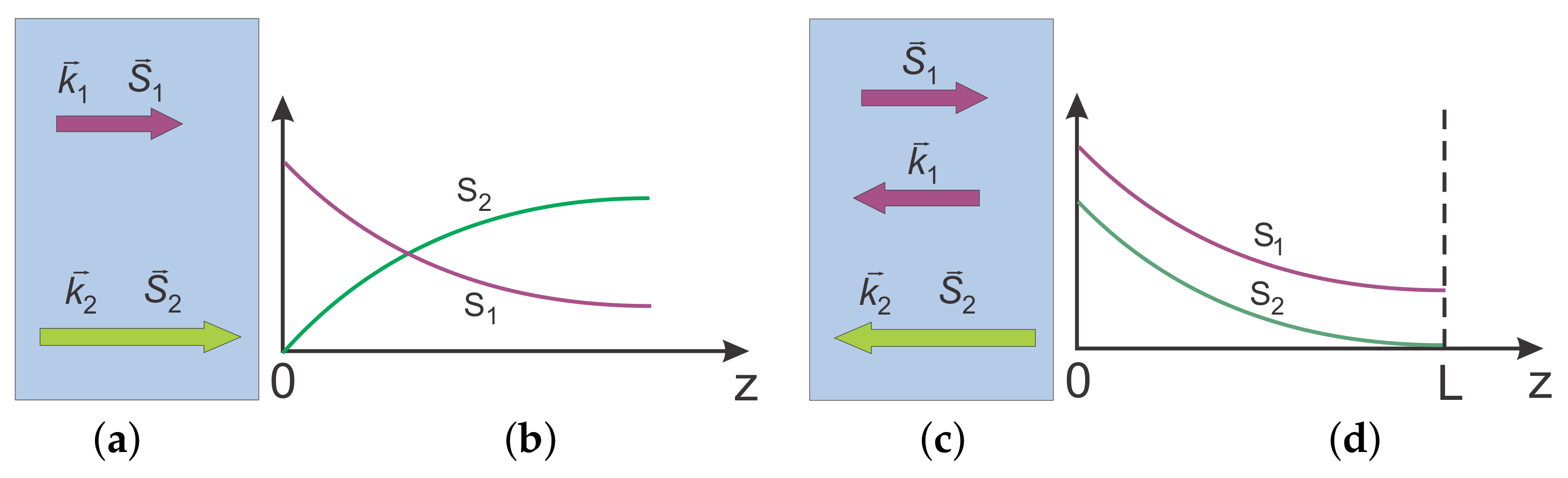
Figure 5.
Differences between second harmonic generation in the ordinary, forward-wave (FW), setting and in the backward-wave (BW) settings. (a) Energy fluxes across the slab for fundamental (descending dash-dotted blue line) and second harmonic (ascending dotted blue line) waves, where both are ordinary forward waves; and for backward-wave fundamental (the descending solid red line) and ordinary second harmonic (the descending dashed red line). . (b) Output transmitted fundamental (the descending blue dash-dotted line) and second harmonic (ascending blue dotted line) at , where both are ordinary forward waves; and transmitted backward-wave fundamental (descending solid red line) flux at and ordinary forward-wave second harmonic contra-propagating flux at (the ascending dashed red line) vs. pump intensity parameter .
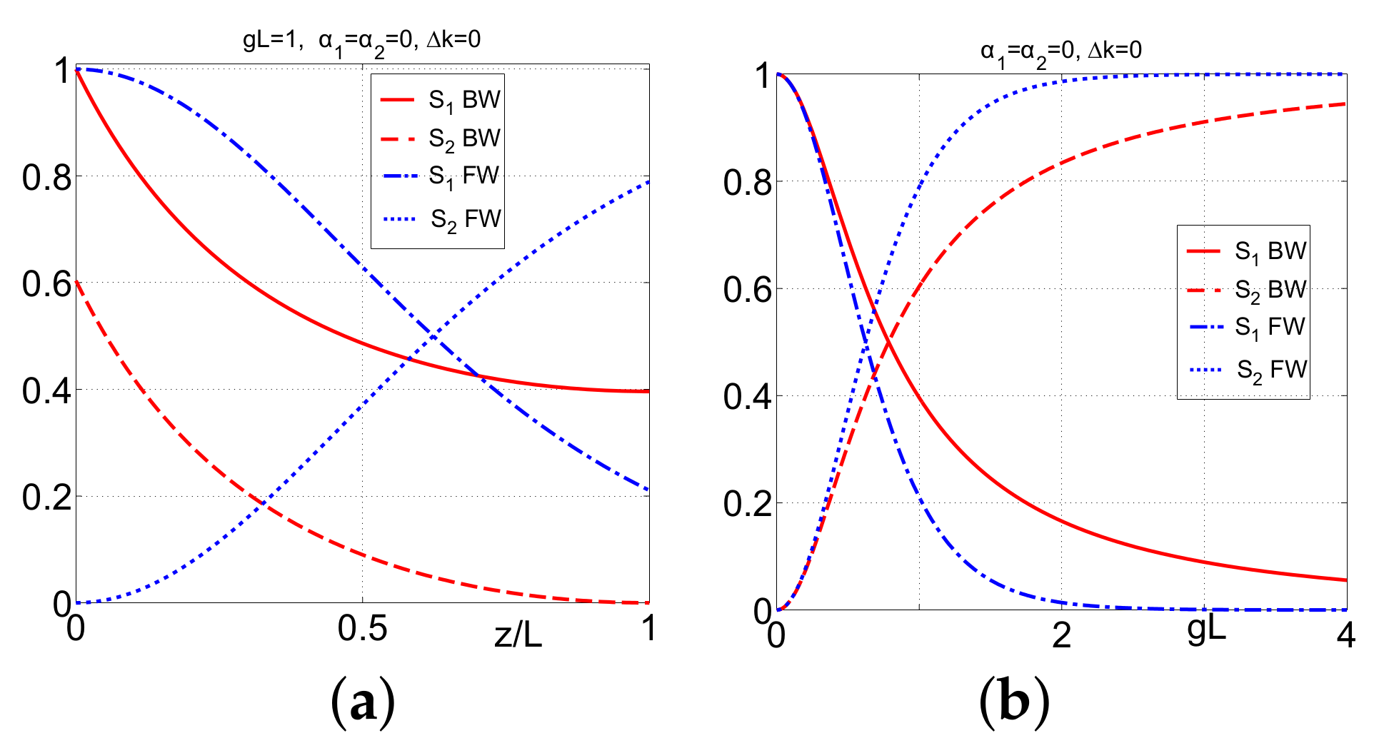
Figure 6.
Comparison of the pulse shapes and the energy conversion for second harmonic generation at the forward-wave (FW) and the backward-wave (BW) settings in a loss-free metamaterial. The length of the input pulse at the fundamental frequency is equal to the metaslab thickness. (a,b) The input rectangular pulse shapes for the fundamental radiation; —for the second harmonic; (c,d) change of the pulse energy at the corresponding frequencies across the slab. Here, , is the fundamental pulse energy, , is the energy (photon) conversion efficiency per pulse.

Figure 7.
Backward-wave second harmonic generation: the effect of pulse width. Here, the input pulse duration is decreased four times as compared with Figure 6a at the same peak intensity. (a) is the pulse shape for the fundamental radiation, and is for the second harmonic; (b) is the fundamental pulse energy, , is the energy (photon) conversion efficiency per pulse, and =4.
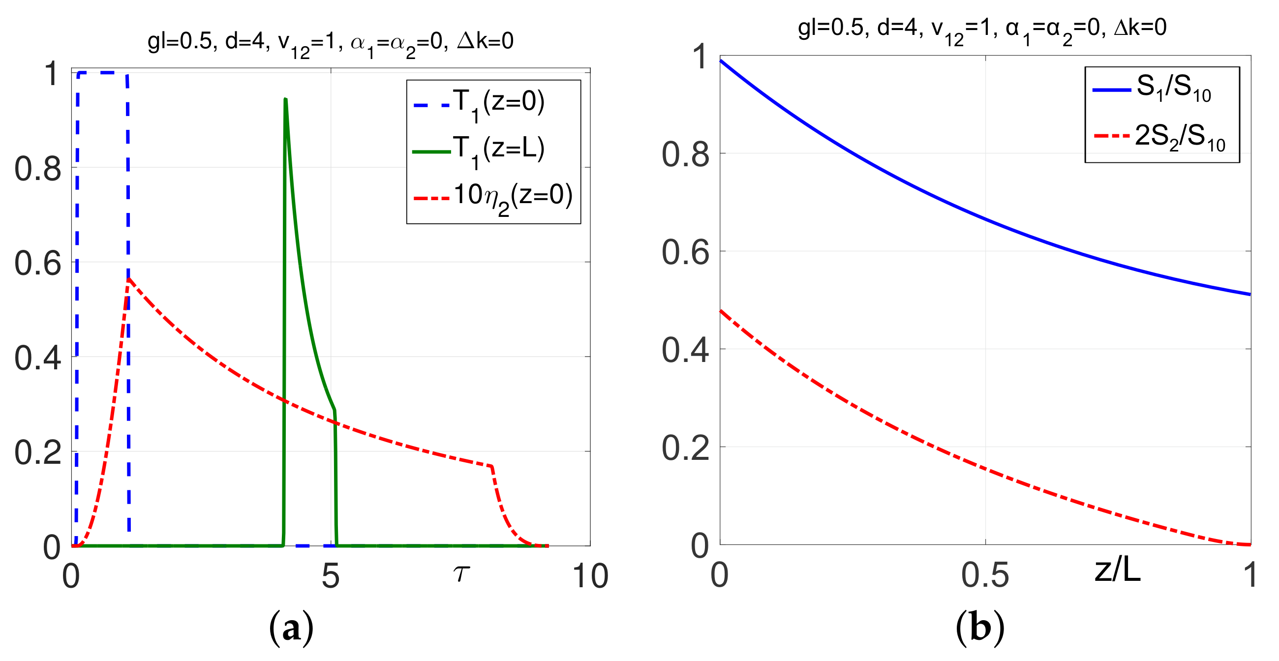
Figure 8.
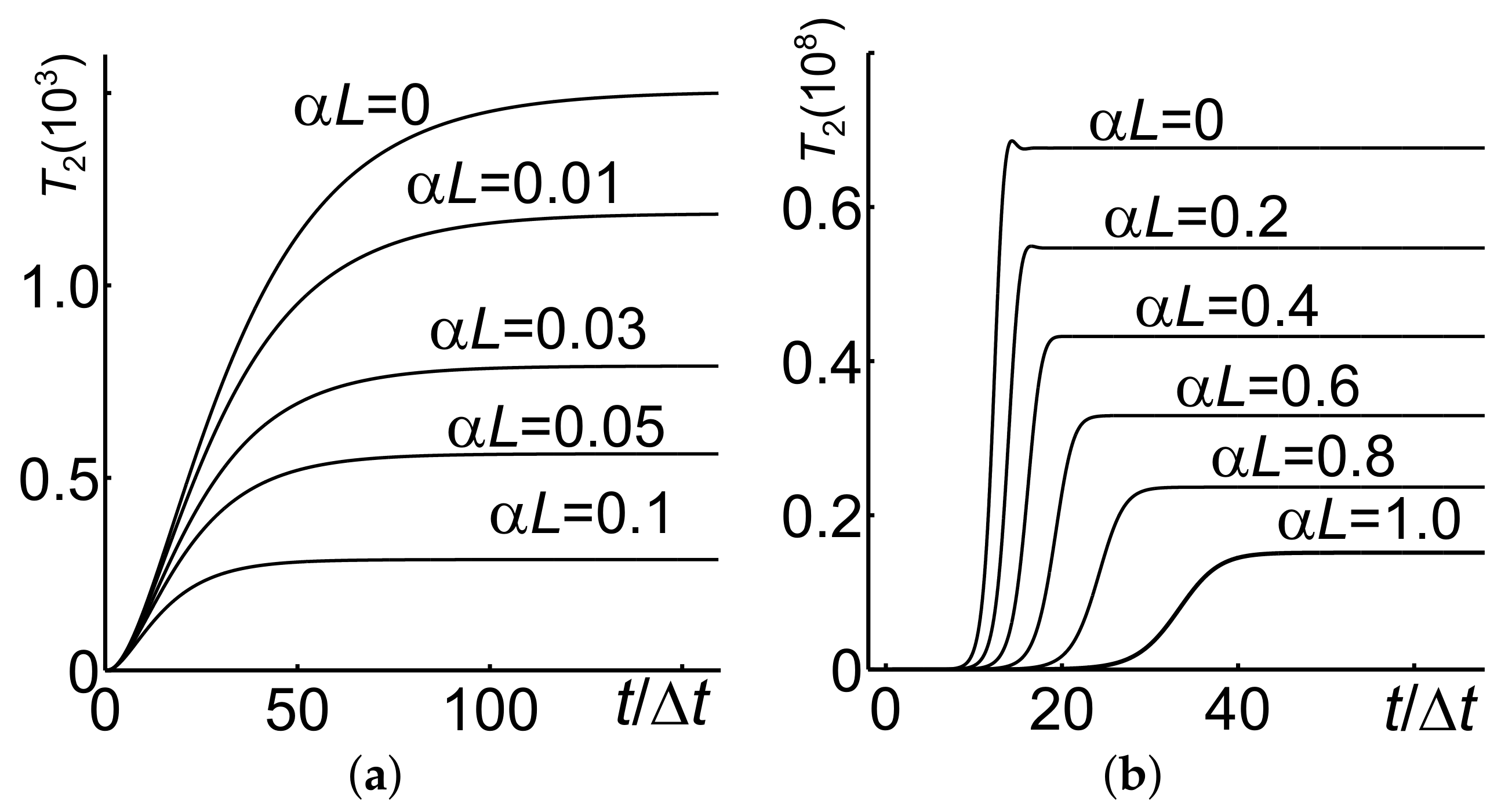
Dependence of the energy conversion efficiency at backward-wave second harmonic generation on the metaslab thickness, intensity, and duration of the pump pulse. (a,b) ; (c,d) ; (a,c) ; (a,d) .
Figure 8.
Dependence of the energy conversion efficiency at backward-wave second harmonic generation on the metaslab thickness, intensity, and duration of the pump pulse. (a,b) ; (c,d) ; (a,c) ; (a,d) .
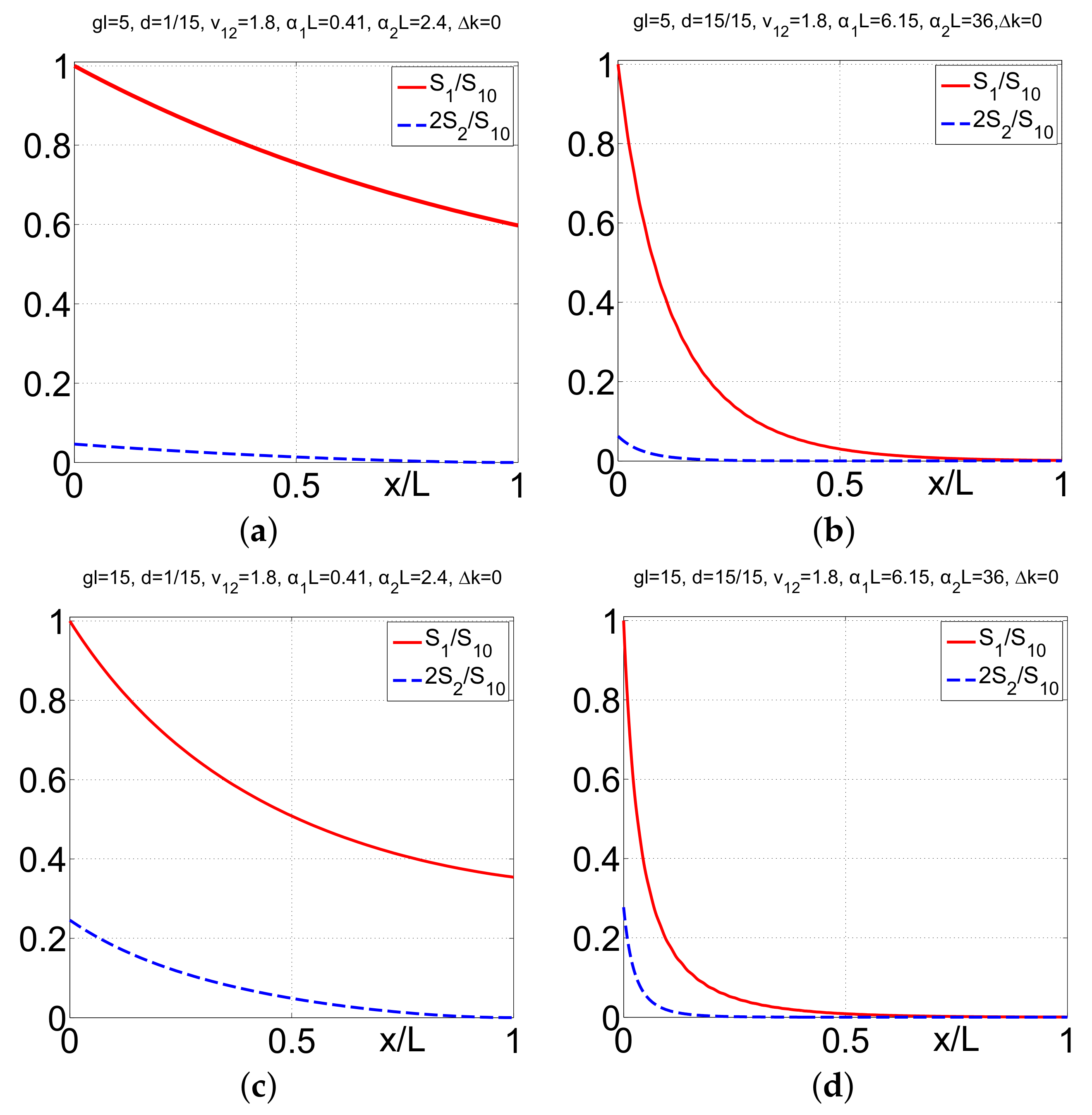
Figure 9.
Ordinary second harmonic generation at all other parametersthe the same as in Figure 8. (a,b) ; (c,d) ; (a,c) ; (a,d) .
Figure 9.
Ordinary second harmonic generation at all other parametersthe the same as in Figure 8. (a,b) ; (c,d) ; (a,c) ; (a,d) .

Figure 10.
Three different options of the proposed nonlinear optical sensors. (a) and are energy fluxes and wavevectors for the ordinary,forward-wave, signal and generated idler; and —backward-wave control field; (b,c) alternative prospective schemes; (b) the NLO sensor amplifies the backward-wave signal traveling against the control beam and frequency up-converts it to the beam directed along the control one; (c) the NLO sensor converts the signal wave traveling along the control field to the frequency-shifted backward-wave idler traveling in the reflection direction against the control beam.

Figure 11.
(a) Difference in transient processes under ordinary (solid lines) and backward-wave (dashed lines) settings. is transmission (optical parametric amplification) of the co-directed seeding signal at the forefront area of the output signal pulse; (b) difference between transient processes in and in nonlinear optical reflectivity (contra-propagating generated idler) for the case of the pulsed input signal and continuous wave pump. (a,b) , , .

Figure 12.
Dependence of the transient processes in the optical parametric amplification on the intensity of the pump field. The dashed line corresponds to three-wave mixing of co-propagating waves. The points correspond to an ordinary signal and contra-propagating idler. The solid lines depict an approximation of the transient optical parametric amplification by the function . , .

Figure 13.
(a) The shape of the signal forefront in a transparent material at pump intensities above the critical input value ; (b) dependence of the transient period on the maximum intensity of the pump field. , .
Figure 13.
(a) The shape of the signal forefront in a transparent material at pump intensities above the critical input value ; (b) dependence of the transient period on the maximum intensity of the pump field. , .

Figure 14.
Effect of absorption on the transients in the optical parametric amplification for two different intensities of the pump field. . . (a) ; (b) .
Figure 14.
Effect of absorption on the transients in the optical parametric amplification for two different intensities of the pump field. . . (a) ; (b) .

Figure 15.
(a) Effect of absorption on the transient period . , , , ; (b) dependence of the duration of the transient period in three-wave mixing on the group velocities of the coupled waves and on their dispersion. , .
Figure 15.
(a) Effect of absorption on the transient period . , , , ; (b) dependence of the duration of the transient period in three-wave mixing on the group velocities of the coupled waves and on their dispersion. , .
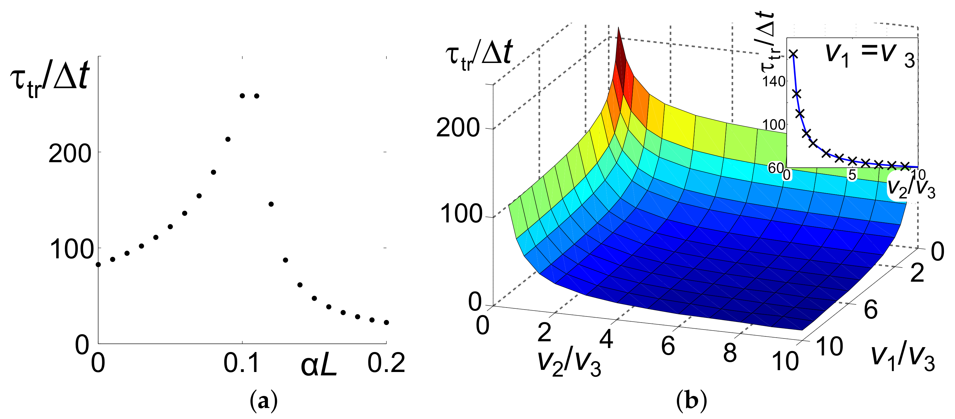
Figure 16.
Dependence of the transient processes in three-wave mixing on the forefront of the output pulses on the dispersion of the group velocities of the coupled waves. , . (a) ; (b) .
Figure 16.
Dependence of the transient processes in three-wave mixing on the forefront of the output pulses on the dispersion of the group velocities of the coupled waves. , . (a) ; (b) .

Figure 17.
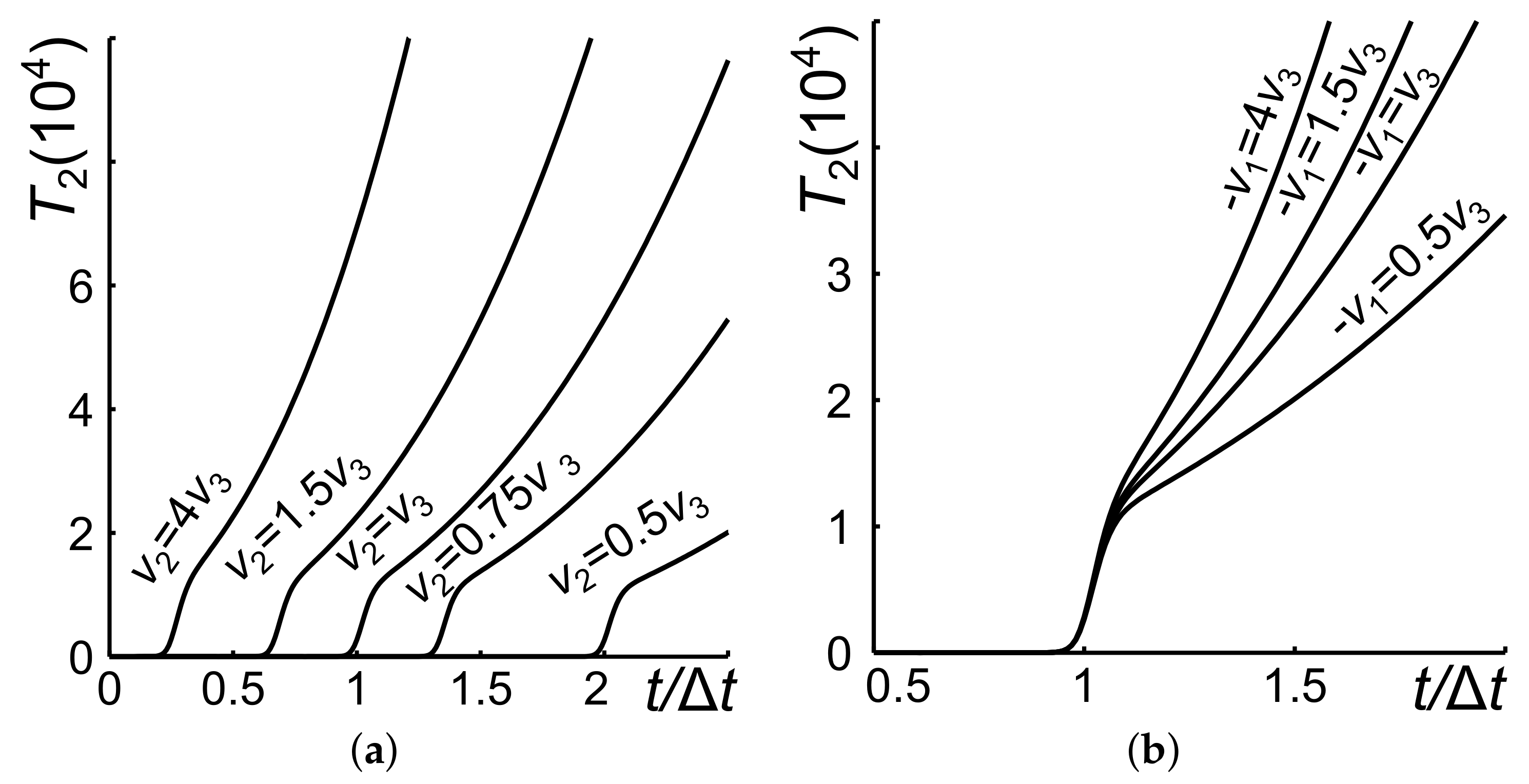
The output normalized signal at (dotted lines) co-directed with a rectangular pump pulse and the output contra-directed idler at (the solid lines) for different values of the pump amplitude . The input signal value is ; is the pump pulse travel time through the slab. (a) ; (b) . Inset: blow up of the peak tip. The dashed lines mark the exit time for the signal pulse rear edge if the pump is not turned on.
Figure 17.
The output normalized signal at (dotted lines) co-directed with a rectangular pump pulse and the output contra-directed idler at (the solid lines) for different values of the pump amplitude . The input signal value is ; is the pump pulse travel time through the slab. (a) ; (b) . Inset: blow up of the peak tip. The dashed lines mark the exit time for the signal pulse rear edge if the pump is not turned on.

Figure 18.
Optical parametric amplification and frequency-shifting nonlinear optical reflectivity vs. intensity of the pump. (a,b) A long pump pulse (quasi- continuous-wave regime). Here, are the transmission factors, and is the input pump maximum. The value represents optical parametric amplification. is nonlinear optical reflectivity. (c,d) The case of a shorter pulse . Here, the transmitted and reflected photon fluxes per pulse are given by the values .
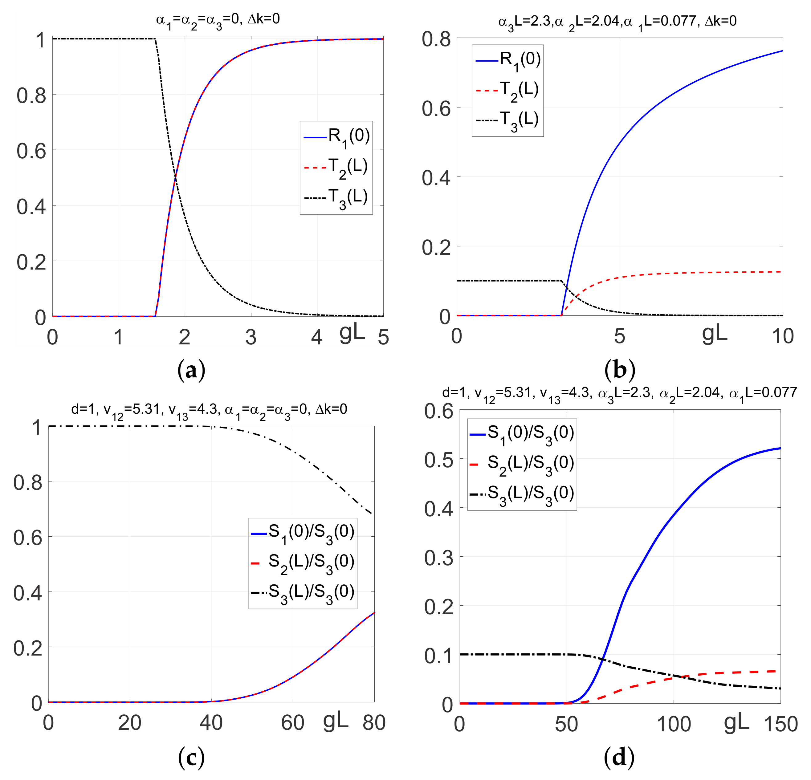
Figure 19.
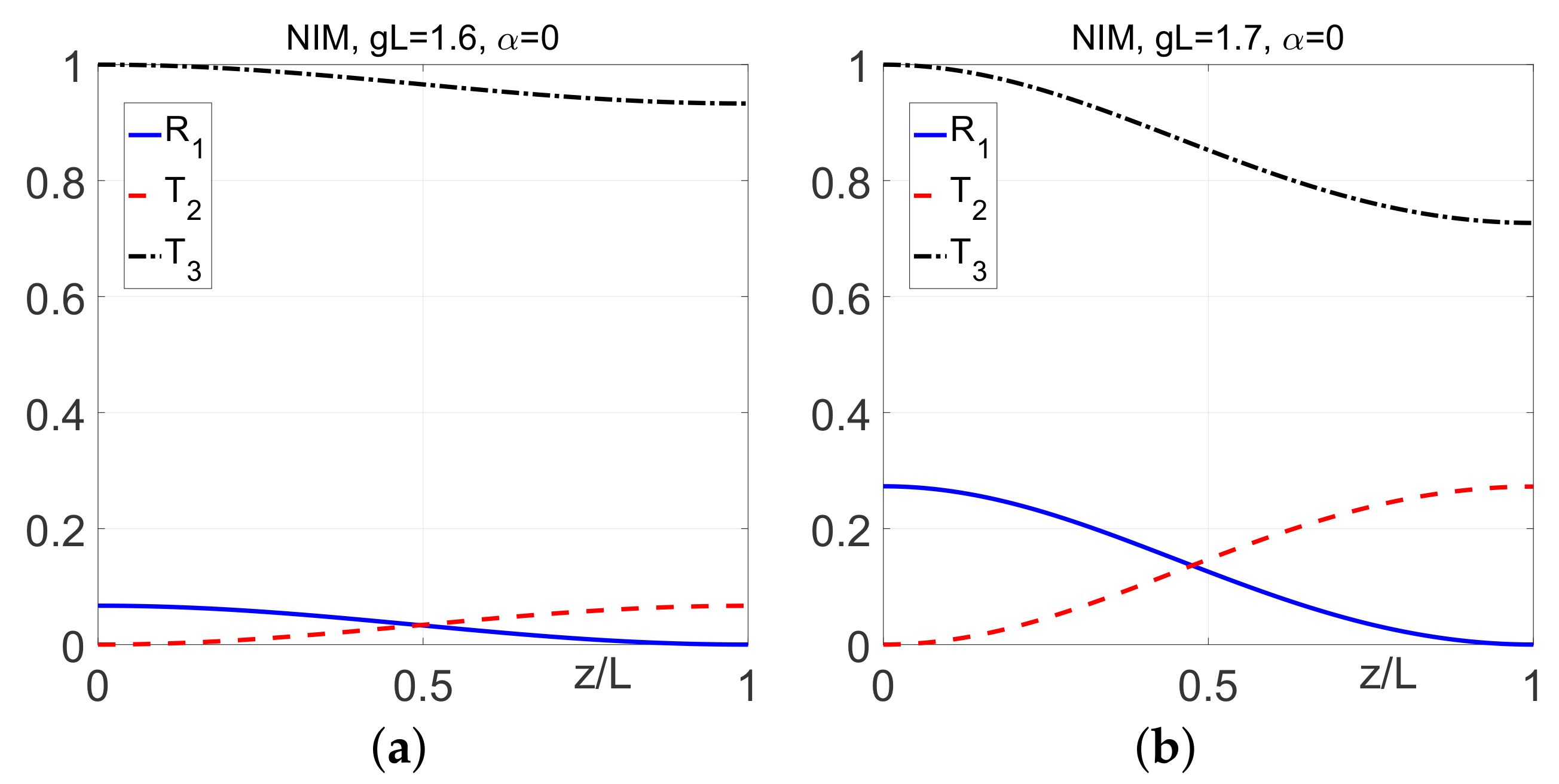
Backward-wave three-wave mixing: the field distribution along the attenuation-free metaslab in the vicinity of the resonance pump intensity. (a) ; (b) .
Figure 19.
Backward-wave three-wave mixing: the field distribution along the attenuation-free metaslab in the vicinity of the resonance pump intensity. (a) ; (b) .

Figure 20.
Output fields vs. intensity of the pump for the ordinary, co-propagating coupling scheme. (a) Attenuation-free material; (b) effect of attenuation dispersion. All attenuation parameters are the same as in Figure 18 (a,b), respectively.
Figure 20.
Output fields vs. intensity of the pump for the ordinary, co-propagating coupling scheme. (a) Attenuation-free material; (b) effect of attenuation dispersion. All attenuation parameters are the same as in Figure 18 (a,b), respectively.

Table 1.
Calculated Metaslab Eigenmodes Data.
| Mode | f, THz | k, m | , m | , m | , m | , m | ||
|---|---|---|---|---|---|---|---|---|
| 1 | 10.43 | 2.186 | 2.26 | 0.988 | 2331 | 28.74 | 19.86 | |
| 2 | 34.95 | 7.325 | 17.8 | 2.61 | 88.2 | 8.58 | 5.93 | |
| 3 | 45.38 | 9.511 | 15.46 | 2.94 | 78.3 | 6.61 | 4.57 |
© 2018 by the authors. Licensee MDPI, Basel, Switzerland. This article is an open access article distributed under the terms and conditions of the Creative Commons Attribution (CC BY) license (http://creativecommons.org/licenses/by/4.0/).
Share and Cite
MDPI and ACS Style
Popov, A.K.; Myslivets, S.A.; Slabko, V.V.; Tkachenko, V.A.; George, T.F. Shaping Light in Backward-Wave Nonlinear Hyperbolic Metamaterials. Photonics 2018, 5, 8. https://doi.org/10.3390/photonics5020008
AMA Style
Popov AK, Myslivets SA, Slabko VV, Tkachenko VA, George TF. Shaping Light in Backward-Wave Nonlinear Hyperbolic Metamaterials. Photonics. 2018; 5(2):8. https://doi.org/10.3390/photonics5020008
Chicago/Turabian StylePopov, Alexander K., Sergey A. Myslivets, Vitaly V. Slabko, Victor A. Tkachenko, and Thomas F. George. 2018. "Shaping Light in Backward-Wave Nonlinear Hyperbolic Metamaterials" Photonics 5, no. 2: 8. https://doi.org/10.3390/photonics5020008
Note that from the first issue of 2016, this journal uses article numbers instead of page numbers. See further details here.