Graphene Plasmonic Waveguides for Mid-Infrared Supercontinuum Generation on a Chip

Abstract

Using perturbation expansion of Maxwell equations with the nonlinear boundary condition, a generic propagation equation is derived to describe nonlinear effects, including spectral broadening of pulses, in graphene surface plasmon (GSP) waveguides. A considerable spectral broadening of an initial 100 fs pulse with $0.5$ mW peak power in a 25 nm wide and 150 nm long waveguide is demonstrated. The generated supercontinuum covers the spectral range from 6 μm to 13 μm.

1. Introduction

Surface plasmon polaritons offer the unique platform to guide and manipulate light at a deeply sub-wavelength scale [1,2,3]. Such tight confinement of light not only enables design of compact plasmonic circuits [3], but also boosts local field intensities and thus allows optical nonlinear processes, such as third harmonic generation [4] and nonlinear switching [5], to occur over short (typically sub-millimeter) propagation distances. However, high ohmic losses in metals impose serious limitations as to nonlinear functionality of plasmonic waveguides. In particular, generation of broad optical spectra (supercontinuum) in a compact plasmonic waveguide remains to be the challenging task.

Recently, graphene has emerged as a promising alternative to noble metals for applications in plasmonics [6,7]. One of the strong advantages of graphene surface plasmons (GSPs) over their conventional metal analogues is the considerably smaller losses [8], particularly in the mid-infrared to terahertz range [7,9]. Several research groups have proposed designs of graphene plasmonic waveguides, as basic building blocks for GSP-based plasmonic circuits [10,11,12,13,14,15,16,17,18]. Graphene is known to possess an exceptionally strong nonlinear optical response [19,20,21], this has been recently confirmed in a number of experimental studies involving frequency mixing, third harmonic generation and z-scan measurements with graphene flakes and in graphene-clad photonic nano-structures [22,23,24,25,26,27,28]. Combined with the unprecedented nano-metre scale light confinement in GSP waveguides, the ultra-strong nonlinearity of graphene can open new routes for design of functional plasmonic circuits.

To describe nonlinear effects, such as frequency mixing and spectral broadening, in graphene waveguides, one needs to take into proper account the purely two-dimensional nature of the optical response of graphene. Recently we developed a perturbation expansion procedure of Maxwell equations, in which graphene is treated as the nonlinear boundary condition [29]. This method has been applied for analysis of self-focusing and switching of monochromatic GSP in single- and bi-layer graphene structures [29,30], and for the description of nonlinear pulse propagation in a graphene-clad dielectric fiber [31]. In this work, the procedure is generalized to the case of a GSP waveguide. The generic pulse propagation equation and the expression for the effective nonlinear coefficient due to graphene are obtained, which enable to analyze nonlinear pulse dynamics in different GSP geometries. As an example, in this work a GSP waveguide formed by a modulation of the graphene Fermi level [17] is considered. We find that in such waveguides the characteristic nonlinear length can be several orders of magnitudes smaller than the propagation length dictated by damping. As the result, one can generate broadband spectra covering more than one frequency octave (6–13 μm) from spectral broadening of a 100 fs pulse with only a few hundred micro-Watt peak power and over propagation distances as short as few hundred nano-metres.

2. Derivation of Pulse Propagation Equation

Consider a GSP waveguide, in which graphene (finite width ribbon or a modulated layer) is located in plane $x=0$, being embedded into a dielectric structure. The waveguide is homogeneous along the propagation direction z, see Figure 1. To describe nonlinear pulse propagation in the structure, it is convenient to use Fourier expansion of the total electric field:

$$\overrightarrow{ℰ}(\overrightarrow{r},t)=\frac{1}{2\sqrt{2\pi }}{\int }_0^{+\infty }\mathbf{E}(\overrightarrow{r},\omega )e^{-i\omega t}d\omega +c.c.$$

(1)

and similar expansions for other fields.

Each Fourier component E solves Maxwell equations:

$$\overrightarrow{\nabla }\times \overrightarrow{\nabla }\times \mathbf{E}=\frac{{\omega }^2}{c^2{ϵ}_0}\mathbf{D}$$

(2)

Optical response of all bulk materials (dielectrics) is incorporated in the displacement vector D. Atom-thick graphene layer is described by means of the surface current J, the corresponding boundary condition is:

$$\overrightarrow{n}\times \left[{\mathbf{H}}_2-{\mathbf{H}}_1\right]=\mathbf{J}$$

(3)

where $\overrightarrow{n}$ is the unit vector normal to the graphene layer and pointing from medium 1 to medium 2, which are on either side of the graphene layer.

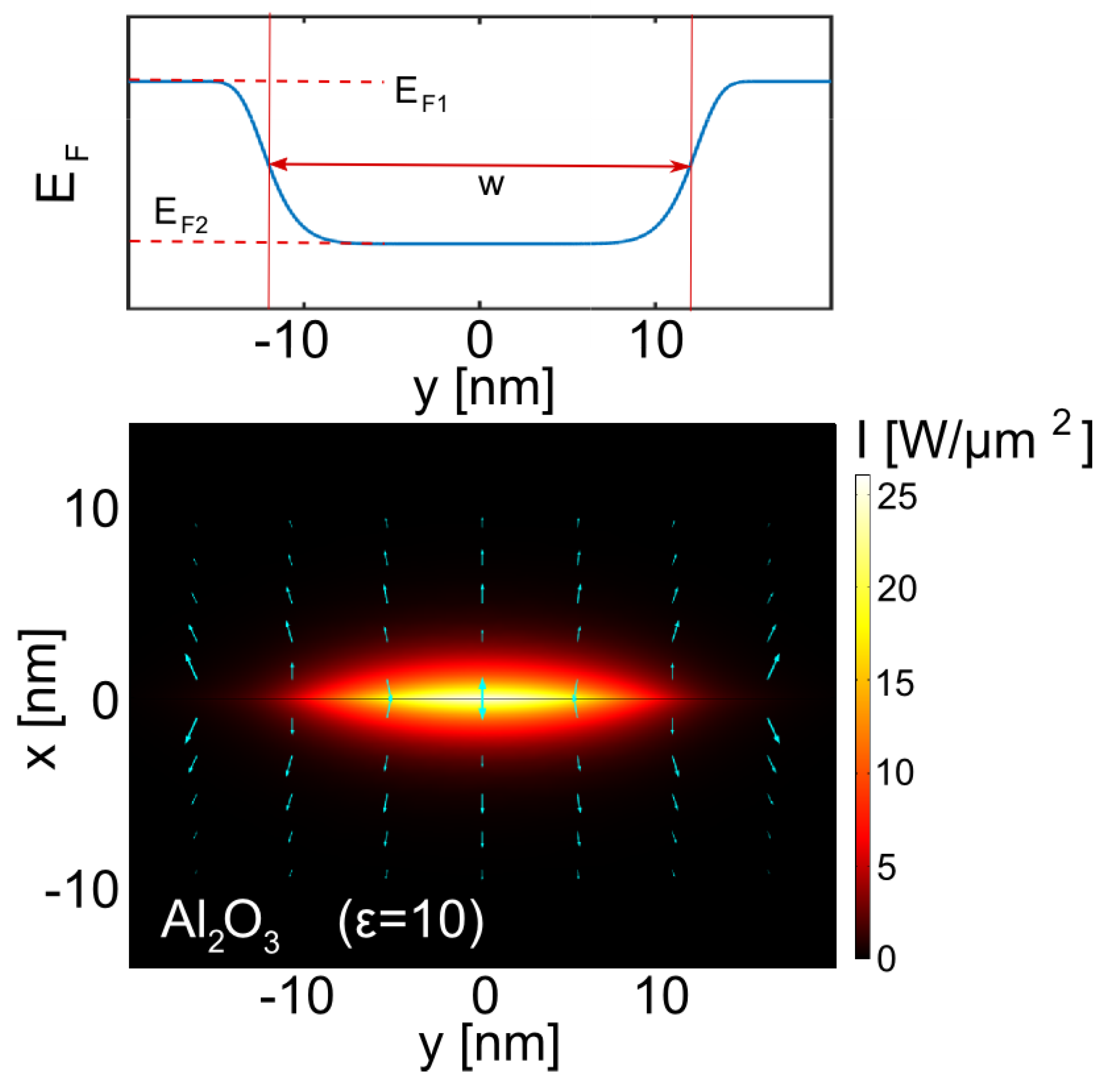
Figure 1. Graphene surface plasmon (GSP) waveguide formed by a modulation of the graphene Fermi energy $E_F$ (see top panel), graphene is embedded into a dielectric (${\mathrm{Al}}_2{\mathrm{O}}_3$) with the relative permittivity $ϵ=10$. The bottom panel illustrates field intensity distribution in the fundamental guided mode at $\lambda =9\mu$m for the case of $E_{F1}=0.25$ eV, $E_{F2}=0.2$ eV and $w=25$ nm, the total power of the mode is $P=1$ mW. Cyan arrows indicate the in-plane direction and magnitude of electric field.

Figure 1. Graphene surface plasmon (GSP) waveguide formed by a modulation of the graphene Fermi energy $E_F$ (see top panel), graphene is embedded into a dielectric (${\mathrm{Al}}_2{\mathrm{O}}_3$) with the relative permittivity $ϵ=10$. The bottom panel illustrates field intensity distribution in the fundamental guided mode at $\lambda =9\mu$m for the case of $E_{F1}=0.25$ eV, $E_{F2}=0.2$ eV and $w=25$ nm, the total power of the mode is $P=1$ mW. Cyan arrows indicate the in-plane direction and magnitude of electric field.

To simplify the derivations, in this work we focus on the cubic (Kerr) nonlinear response of graphene, leaving the polarization due to the dielectrics to be purely linear. It is a straightforward exercise to extend the described below procedure and include nonlinear dielectric polarization. At the same time, for GSPs in planar structures the relative contribution of dielectrics to the overall nonlinearity has been demonstrated to be minuscule [29], which justifies the simplification adopted here. We also neglect any effects associated with third harmonic generation, since they require specially engineered phase matching. In other words, we assume that the pulse spectrum is narrow enough to not accommodate the third harmonic. For the same reason, possible second harmonic generation and associated effects due to a non-zero second order nonlinear graphene conductivity, arising from spatial dispersion near the plasmon resonance [21], are also neglected. Under these assumptions, the Fourier components of the displacement vector and the graphene current are:

$$\begin{array}{c}\hfill \mathbf{D}\left(\omega \right)={ϵ}_0ϵ\mathbf{E}\left(\omega \right)\end{array}$$

(4)

$$\begin{array}{c}\hfill \mathbf{J}\left(\omega \right)={\widehat{\sigma }}_1^{\left(1\right)}\mathbf{E}\left(\omega \right)+{\mathbf{J}}_{nl}(\mathbf{E}\left({\omega }_1),\mathbf{E}\left({\omega }_2\right),\mathbf{E}\left({\omega }_3\right)\right)\end{array}$$

(5)

$$\begin{array}{c}\hfill {\mathbf{J}}_{nl}\left({\mathbf{E}}_1,{\mathbf{E}}_2,{\mathbf{E}}_3\right)=\frac{1}{8\pi }{\int \int }_0^{\infty }{\widehat{\sigma }}^{\left(3\right)}⋮{\mathbf{E}}_1{\mathbf{E}}_2^{*}{\mathbf{E}}_{3}d{\omega }_{1}d{\omega }_2\end{array}$$

(6)

$$\begin{array}{c}\hfill {\omega }_3=\omega -{\omega }_1+{\omega }_2\end{array}$$

(7)

In the above expression for ${\mathbf{J}}_{nl}$ vertical dots stand for tensor product: $\mathbf{a}=\widehat{O}⋮\mathbf{b}\mathbf{c}\mathbf{d}$, $a_i={\widehat{O}}_{ijkl}{b}_j{c}_k{d}_l$. For excitation frequencies below the single-photon absorption resonance in graphene, $\hslash \omega <2E_F$, the structure of the third-order nonlinear conductivity tensor can be approximated as [19,32]: ${\widehat{\sigma }}_{ipjs}^{\left(3\right)}={\sigma }_3\left[{\delta }_{ip}{\delta }_{js}+{\delta }_{ij}{\delta }_{ps}+{\delta }_{is}{\delta }_{pj}\right]$, ${\delta }_{ij}$ is the Kronecker’s delta, the indexes $i,p,j,s$ are each from the subset of in-plane coordinates $(y,z)$. Also, the 2D symmetry of graphene and the assumption of zero transversal current $J_x=0$ still permit six additional non-zero tenzor components ${\widehat{\sigma }}_{jjxx}^{\left(3\right)}={\widehat{\sigma }}_{jxjx}^{\left(3\right)}={\widehat{\sigma }}_{jxxj}^{\left(3\right)}=\widetilde{{\sigma }_3}$, $j=y,z$. In absence of external magnetic fields, linear conductivity tensor has only two diagonal non-zero components: ${\widehat{\sigma }}_{ii}^{\left(1\right)}={\sigma }_1$, $i=y,z$.

The relative dielectric permittivity $ϵ=ϵ(x,y)$, together with the y-dependent tensors of linear and nonlinear graphene conductivity, define the transverse geometry of the waveguide, cf. Figure 1.

2.1. Perturbation Expansion of Nonlinear Maxwell Equations

It is convenient to decompose the surface current as $\mathbf{J}={\mathbf{J}}_0+{\mathbf{J}}_p$, so that the solution of Maxwell equations with ${\mathbf{J}}_0$ gives the linear guided mode of the structure, while ${\mathbf{J}}_p$ is treated as a perturbation and contains the nonlinear term ${\mathbf{J}}_{nl}$ and damping due to non-zero real part of ${\sigma }_1$ (one can formally include the damping term into the leading order ${\mathbf{J}}_0$ and consider quasi-guided modes with complex propagation constants, see e.g., Reference [33], however it is more convenient to work with real guided modes).

Developing perturbation expansion, we introduce a dummy small parameter s assuming ${\mathbf{J}}_p\sim s^{3/2}$. Each Fourier component of the electric field is expanded in the perturbation series as:

$$\mathbf{E}=s^{1/2}{N}_{\omega }^{-1/2}{A}_{\omega }\left(sz\right){\mathbf{e}}_{\omega }(x,y)e^{i\beta z}+s^{3/2}{\mathbf{E}}_1(x,y,sz)e^{i\beta z}+O\left(s^{5/2}\right)$$

(8)

and a similar expansion for the magnetic field is assumed. Here ${\mathbf{e}}_{\omega }$ is the mode of a given structure, $\beta =\beta \left(\omega \right)$ is the corresponding propagation constant, $N_{\omega }$ is an optional normalization factor. We consider a single-mode situation, neglecting any nonlinear coupling to possible higher order modes of the waveguide, which is inefficient due to the high mismatch between propagation constants of different modes.

Following substitution of the ansatz in Equation (8) into Maxwell equations, in the lowest order of the small parameter, $O\left(s^{1/2}\right)$ the eigenvalue problem is obtained:

$$\begin{array}{ccc}\hfill \widehat{L}\left(\beta \right){\mathbf{e}}_{\omega }& =& 0,\hfill \end{array}$$

(9)

$$\begin{array}{ccc}\hfill \widehat{L}\left(\beta \right)& =& \left[\begin{array}{ccc}{q}^2-{\partial }_y^2& {\partial }_{xy}^2& i\beta {\partial }_x\\ {\partial }_{xy}^2& q^2-{\partial }_x^2& i\beta {\partial }_y\\ i\beta {\partial }_x& i\beta {\partial }_y& -ϵk^2-{\partial }_x^2-{\partial }_y^2\end{array}\right]\hfill \end{array}$$

(10)

where $q^2={\beta }^2-ϵk^2$. The boundary conditions for the mode ${\mathbf{e}}_{\omega }$ are:

$$\begin{array}{c}\hfill \Delta \left[e_{\omega ,z}\right]=0,\Delta \left[e_{\omega ,y}\right]=0\end{array}$$

(11)

$$\begin{array}{c}\hfill \Delta [{\partial }_y{e}_{\omega ,x}-{\partial }_x{e}_{\omega ,y}]=\frac{-i\omega }{{ϵ}_0{c}^2}{J}_{0y}=\frac{{\sigma }_1^{\left(I\right)}}{{ϵ}_0{c}^2}{e}_{\omega ,y}\end{array}$$

(12)

$$\begin{array}{c}\hfill \Delta [i\beta e_{\omega ,x}-{\partial }_x{e}_{\omega ,z}]=\frac{-i\omega }{{ϵ}_0{c}^2}{J}_{0z}=\frac{{\sigma }_1^{\left(I\right)}}{{ϵ}_0{c}^2}{e}_{\omega ,z}\end{array}$$

(13)

where ${\sigma }_1^{\left(I\right)}={\sigma }_1^{\left(I\right)}\left(y\right)=\mathrm{Im}\left({\sigma }_1\right)$ is the imaginary part of linear graphene conductivity, the operator Δ is defined as:

$$\begin{array}{ccc}\hfill \Delta \left[f\right(x\left)\right]& =& \underset{\delta \to 0}{lim}\left(f(-\delta )-f\left(\delta \right)\right)\hfill \end{array}$$

(14)

Solving the eigenvalue problem in Equation (9), we obtain the modal profile $\mathbf{e}(x,y)$ and the dispersion of the mode $\beta \left(\omega \right)$.

It is convenient to choose the normalization factor $N_{\omega }$ as:

$$\begin{array}{c}\hfill N_{\omega }=\frac{1}{4}{\int \int }_{-\infty }^{+\infty }({\mathbf{e}}_{\omega }\times {\mathbf{h}}_{\omega }^{*}){\widehat{e}}_{z}dxdy+c.c.\end{array}$$

(15)

where ${\widehat{e}}_z$ is the unit vector along z-axis. With this normalization, in the lowest order of the small parameter, $O\left(s\right)$, the total energy carried by a pulse along the waveguide is given by:

$$W={\int \int \int }_{-\infty }^{\infty }\left(ℰ\times \mathscr{H}\right){\widehat{e}}_{z}dxdydt={\int }_0^{\infty }{\left|A_{\omega }\right|}^{2}d\omega$$

(16)

Here we assume that the pulse is localized in time, and the mode ${\mathbf{e}}_{\omega }(x,y)$ is localized in the transversal plane at all frequencies, so that the integrals in the above expression converge.

In the next order of the perturbation expansion of Maxwell equations, $O\left(s^{3/2}\right)$, we obtain:

$$\begin{array}{ccc}\hfill \widehat{L}{\mathbf{E}}_1& =& \mathbf{R}\left({\partial }_z{A}_{\omega }\right)\hfill \end{array}$$

(17)

$$\begin{array}{ccc}\hfill \mathbf{R}& =& N_{\omega }^{-1/2}{\partial }_z{A}_{\omega }{\widehat{M}}_{xy}{\mathbf{e}}_{\omega }\hfill \end{array}$$

(18)

$$\begin{array}{ccc}\hfill {\widehat{M}}_{xy}& =& \left[\begin{array}{ccc}2i\beta & 0& -{\partial }_x\\ 0& 2i\beta & -{\partial }_y\\ -{\partial }_x& -{\partial }_y& 0\end{array}\right]\hfill \end{array}$$

(19)

together with the boundary conditions:

$$\begin{array}{c}\hfill \Delta \left[E_{1z}\right]=0,\Delta \left[E_{1y}\right]=0\end{array}$$

(20)

$$\begin{array}{c}\hfill \Delta [{\partial }_y{E}_{1x}-{\partial }_x{E}_{1y}]=\frac{-i\omega }{{ϵ}_0{c}^2}{J}_{py}\end{array}$$

(21)

$$\begin{array}{c}\hfill \Delta [N_{\omega }^{-1/2}{\partial }_z{A}_{\omega }{e}_{\omega ,x}+i\beta E_{1x}-{\partial }_x{E}_{1z}]=\frac{-i\omega }{{ϵ}_0{c}^2}{J}_{pz}\end{array}$$

(22)

where the perturbation current ${\mathbf{J}}_p$ combines damping due to non-zero real part ${\sigma }_1^{\left(R\right)}=\mathrm{Re}\left({\sigma }_1\right)$ and the nonlinear current:

$$\begin{array}{ccc}\hfill {\mathbf{J}}_p& =& N_{\omega }^{-1/2}{A}_{\omega }{\widehat{\sigma }}_1^{\left(R\right)}{\mathbf{e}}_{\omega }+{\mathbf{J}}_{nl}\left(N_{{\omega }_1}^{-1/2}{A}_{{\omega }_1}{\mathbf{e}}_{{\omega }_1},N_{{\omega }_2}^{-1/2}{A}_{{\omega }_2}{\mathbf{e}}_{{\omega }_2},N_{{\omega }_3}^{-1/2}{A}_{{\omega }_3}{\mathbf{e}}_{{\omega }_3}\right)e^{i\Delta \beta z}\hfill \end{array}$$

(23)

$$\begin{array}{ccc}\hfill \Delta \beta & =& \beta \left({\omega }_1\right)+\beta \left({\omega }_3\right)-\beta \left({\omega }_2\right)-\beta \left(\omega \right)\hfill \end{array}$$

(24)

Next, we project Equation (17) onto the mode ${\mathbf{e}}_{\omega }$ to obtain:

$$〈{\mathbf{e}}_{\omega }\left|\widehat{L}\right|{\mathbf{E}}_1〉=〈{\mathbf{e}}_{\omega }|\mathbf{R}〉$$

(25)

where $〈\mathbf{a}|\mathbf{b}〉={\int \int }_{-\infty }^{\infty }\left({\mathbf{a}}^{*}·\mathbf{b}\right)dxdy$. It is important to note that ${\mathbf{e}}_{\omega }$ and ${\mathbf{E}}_1$ satisfy different boundary conditions, Equations (11–13) and (20–22), respectively. This removes the self-adjoint property of the operator $\widehat{L}$, so that $〈{\mathbf{e}}_{\omega }\left|\widehat{L}\right|{\mathbf{E}}_1〉\ne {〈{\mathbf{E}}_1\left|\widehat{L}\right|{\mathbf{e}}_{\omega }〉}^{*}$. To proceed, we split integration in x in the l.h.s. of Equation (25) as ${\int }_{-\infty }^{\infty }dx={\int }_{-\infty }^{0}dx+{\int }_0^{\infty }dx$ and take the resulting integrals by parts. Following some algebra, it is possible to show that [29]:

$$\begin{array}{ccc}\hfill 〈{\mathbf{e}}_{\omega }\left|\widehat{L}\right|{\mathbf{E}}_1〉& =& {〈{\mathbf{E}}_1\left|\widehat{L}\right|{\mathbf{e}}_{\omega }〉}^{*}-\frac{i\omega }{{ϵ}_0{c}^2}{\int }_{-\infty }^{\infty }\left[J_{py}{e}_{\omega ,y}^{*}+J_{pz}{e}_{\omega ,z}^{*}\right]dy\hfill \\ & & -N_{\omega }^{-1/2}{\partial }_z{A}_{\omega }{\int }_{-\infty }^{\infty }\Delta \left[e_{\omega ,x}{e}_{\omega ,z}^{*}\right]dy\hfill \end{array}$$

(26)

Computing integrals in the r.h.s. of Equation (25) we obtain:

$$\begin{array}{ccc}\hfill 〈{\mathbf{e}}_{\omega }|\mathbf{R}〉& =& N_{\omega }^{-1/2}{\partial }_z{A}_{\omega }\left(2i\beta \underset{-\infty }{\overset{\infty }{\int \int }}{\left|{\mathbf{e}}_{\omega }\right|}^{2}dxdy-{\int }_{-\infty }^{\infty }\Delta \left[e_{\omega ,x}^{*}{e}_{\omega ,z}\right]dy\right)\hfill \end{array}$$

(27)

Taking into account that $\widehat{L}{\mathbf{e}}_{\omega }=0$, and combining the results in Equations (26) and (27), the propagation equation for the modal amplitudes $A_{\omega }$ is obtained:

$$\begin{array}{c}\hfill i{\partial }_z{A}_{\omega }=-i{\alpha }_{\omega }{A}_{\omega }-e^{i\Delta \beta z}\frac{1}{2\pi }\underset{0}{\overset{\infty }{\int \int }}{\gamma }_{\omega {\omega }_1{\omega }_2{\omega }_3}{A}_{{\omega }_1}{A}_{{\omega }_2}^{*}{A}_{{\omega }_3}d{\omega }_{1}d{\omega }_2\end{array}$$

(28)

where the damping and nonlinear coefficients are given by:

$$\begin{array}{ccc}\hfill {\alpha }_{\omega }& =& \frac{1}{4N_{\omega }}{\int }_{-\infty }^{+\infty }{\sigma }_1^{\left(R\right)}{\left({\mathbf{e}}_{\omega }{\mathbf{e}}_{\omega }^{*}\right)}_{\eta 0}dy\hfill \end{array}$$

(29)

$$\begin{array}{ccc}\hfill {\gamma }_{\omega {\omega }_1{\omega }_2{\omega }_3}& =& \frac{1}{16\sqrt{N_{\omega }{N}_{{\omega }_1}{N}_{{\omega }_2}{N}_{{\omega }_3}}}\times \hfill \\ & & {\int }_{-\infty }^{+\infty }i{\sigma }_3\left[{\left({\mathbf{e}}_{{\omega }_1}{\mathbf{e}}_{{\omega }_2}^{*}\right)}_{\eta }{\left({\mathbf{e}}_{{\omega }_3}{\mathbf{e}}_{\omega }^{*}\right)}_{\eta 0}+{\left({\mathbf{e}}_{{\omega }_3}{\mathbf{e}}_{{\omega }_2}^{*}\right)}_{\eta }{\left({\mathbf{e}}_{{\omega }_1}{\mathbf{e}}_{\omega }^{*}\right)}_{\eta 0}+{\left({\mathbf{e}}_{{\omega }_1}{\mathbf{e}}_{{\omega }_3}\right)}_{\eta }{\left({\mathbf{e}}_{{\omega }_2}^{*}{\mathbf{e}}_{\omega }^{*}\right)}_{\eta 0}\right]dy\hfill \end{array}$$

(30)

In the above expressions the deformed scalar products are introduced: ${\left(\mathbf{a}\mathbf{b}\right)}_{\eta }=\eta a_x{b}_x+a_y{b}_y+a_z{b}_z$, ${\left(\mathbf{a}\mathbf{b}\right)}_{\eta 0}=a_y{b}_y+a_z{b}_z$. The deformation factor $\eta ={\tilde{\sigma }}_3/{\sigma }_3$ characterizes the relative impact of the orthogonal field component on the induced current in the graphene layer.

In the derivation of Equation (28) the following identity was used:

$$\begin{array}{ccc}\hfill N_{\omega }& =& \frac{{ϵ}_0{c}^2}{2\omega }\left\{\beta {\int \int }_{-\infty }^{\infty }{\left|{\mathbf{e}}_{\omega }\right|}^{2}dxdy+\mathrm{Im}\left({\int }_{-\infty }^{\infty }\Delta \left[e_{\omega ,x}{e}_{\omega ,z}^{*}\right]dy\right)\right\}\hfill \end{array}$$

(31)

which can be obtained directly from Equation (15) by using the relationship between magnetic ${\mathbf{h}}_{\omega }$ and electric ${\mathbf{e}}_{\omega }$ fields of the guided mode.

2.2. Pulse Propagation Equation

The propagation Equation (28) takes into full account material and geometrical dispersion of linear and nonlinear coefficients. However, numerical propagation within this model is a computationally challenging task. For certain applications, including propagation of a relatively narrow-band pulse (with $\Delta \omega /{\omega }_0\ll 1$, where ${\omega }_0$ is the central frequency of the pulse), it is possible to neglect the dispersion of nonlinear coefficients and replace ${\gamma }_{\omega {\omega }_1{\omega }_2{\omega }_3}$ in Equation (28) with a constant coefficient evaluated at the reference frequency (A more accurate procedure, which still allows the preservation of the dispersion of nonlinearity, is based on the factorization of the nonlinear coefficients and is described in detai in Reference [34]):

$${\gamma }_{\omega {\omega }_1{\omega }_2{\omega }_3}\approx {\gamma }_{{\omega }_0{\omega }_0{\omega }_0{\omega }_0}=\gamma$$

(32)

Furthermore, assuming that the spectrum of the pulse is localized in a vicinity of ${\omega }_0$, we can consider the analytical extension of the spectrum $A_{\omega }$ onto the negative frequency half-axis, and the corresponding complex time-domain function defined as:

$$A(z,t)=\frac{1}{\sqrt{2\pi }}{\int }_{-\infty }^{\infty }{A}_{\omega }{e}^{-i\omega t}d\omega$$

(33)

Let us introduce the pulse envelope function $\Psi (z,t)$:

$$\Psi (z,t)=\frac{1}{\sqrt{2\pi }}{\int }_{-\infty }^{\infty }{A}_{\delta }exp\left[i\left(\beta -{\beta }_0-\frac{\delta }{v_g}\right)z\right]e^{-i\delta t}d\delta$$

(34)

where $A_{\delta }=A_{\omega -{\omega }_0}$ is the shifted spectrum of the pulse, ${\beta }_0=\beta \left({\omega }_0\right)$ and $v_g^{-1}=\partial \beta /\partial \omega \left({\omega }_0\right)$ are the propagation constant and the inverse group velocity at the reference frequency, respectively. It is easy to see, that the relationship between $\Psi (z,t)$ and $A(z,t)$ is:

$$A(z,t)=\Psi \left(z,\tau =t-z/v_g\right)e^{-i{\omega }_{0}t}{e}^{i({\beta }_0-\beta )z}$$

(35)

Extending integration in the r.h.s. of Equation (28) onto negative frequency domain, we thus can re-write the propagation equation in terms of the spectral amplitudes ${\Psi }_{\delta }$ of the envelope function $\Psi (z,t)$ as follows:

$${\partial }_z{\Psi }_{\delta }=\left(i{\tilde{\beta }}_{\delta }-{\alpha }_{\delta }\right){\Psi }_{\delta }+i\gamma ℱ{\left\{{|\Psi |}^2\Psi \right\}}_{\delta }$$

(36)

where ${\tilde{\beta }}_{\delta }=\beta -{\beta }_0-\delta /v_g$ and $ℱ{\left\{f\left(t\right)\right\}}_{\delta }$ is the Fourier amplitude of the function $f\left(t\right)$ at frequency δ. It is easy to see that:

$$ℱ{\left\{{|\Psi |}^2\Psi \right\}}_{\delta }=\frac{1}{2\pi }{\int \int }_{-\infty }^{\infty }{\Psi }_{{\delta }_1}{\Psi }_{{\delta }_2}^{*}{\Psi }_{\delta -{\delta }_1+{\delta }_2}d{\delta }_{1}d{\delta }_2$$

(37)

The derived Equation (36) is the spectral representation of the renowned generalized Nonlinear Schrödinger Equation, widely used for the description of pulse propagation in nonlinear waveguides and fibres [35]. Unlike the Equation (28), the reduced model in Equation (36) is easy to integrate numerically with the help of the well-developed split-step method, whereby the nonlinear part is evaluated in time domain [35]. Note that the definition of the pulse envelope function Ψ in Equation (34) does not involve any additional renormalizations. In particular, the pulse energy W, Equation (16), is computed as:

$$W={\int }_{-\infty }^{\infty }|{\Psi }_{\delta }{\left(z\right)|}^{2}d\delta ={\int }_{-\infty }^{\infty }{|\Psi (z,t)|}^{2}dt$$

(38)

The derived propagation Equation (28) and its simplified version in Equation (36), together with the set of coefficients defined in Equations (29) and (30) represent a comprehensive set of tools to analyze nonlinear pulse dynamics and frequency conversion processes in any GSP waveguide geometry.

3. Spectral Broadening in a GSP Waveguide

In this section we consider a particular example of a GSP waveguide created by a local modulation of the graphene Fermi level [17], see Figure 1. The graphene is embedded into a dielectric matrix, for which the constant permittivity $ϵ=10$ was assumed.

The linear conductivity of graphene is given by [36]:

$$\begin{array}{ccc}\hfill {\sigma }_1& =& \frac{i2e^2{k}_{B}T}{\pi {\hslash }^2(\omega +i{\tau }^{-1})}ln\left[2cosh\left(\frac{E_F}{2k_{B}T}\right)\right]\hfill \\ & & +\frac{e^2}{4\hslash }\left[G\left(\frac{\omega }{2}\right)+i\frac{2\omega }{\pi }{\int }_0^{+\infty }\frac{G({\omega }^{\prime }/2)-G(\omega /2)}{{\omega }^2-{\left({\omega }^{\prime }\right)}^2}d{\omega }^{\prime }\right]\hfill \end{array}$$

(39)

$$\begin{array}{ccc}\hfill G\left(\omega \right)& =& \frac{sinh\left[\hslash \omega /\left(k_{B}T\right)\right]}{cosh\left[E_F/\left(k_{B}T\right)\right]+cosh\left[\hslash \omega /\left(k_{B}T\right)\right]}\hfill \end{array}$$

For frequencies below the optical phonon resonance $\hslash \omega <0.2eV$ (λ > 6 μm) and below the absorption threshold $\hslash \omega <2E_F$ the relaxation time due to impurities is typically below 1 ps [6,7]. In the simulations we used $\tau =0.5$ ps and $T=300$ K.

The profile of Fermi energy, shown in the top panel of Figure 1, was modeled as:

$$E_F\left(y\right)=E_{F1}+(E_{F2}-E_{F1})exp\left[-{(2y/w)}^{10}\right]$$

(40)

Taking $E_{F1}=0.25$ eV and $E_{F2}=0.2$ eV, this modulation corresponds to the variation of conductivity from ${\sigma }_{1,hi}^{\left(I\right)}$ = 1.291 × 10${}^{-4}$ S to ${\sigma }_{1,lo}^{\left(I\right)}$ = 0.973 × 10${}^{-4}$ S at ${\lambda }_0=$9 μm. While the propagation constant of GSP on a homogeneous graphene is inversely proportional to ${\sigma }_1$ [6,7]:

$${\beta }_{GSP}\approx \frac{2{ϵ}_0ϵc}{-i{\sigma }_1}$$

(41)

such a local decrease of the conductivity effectively forms a waveguide for plasmons [17].

In Figure 2 linear and nonlinear parameters for waveguides of different widths w are summarized. The effective index of the mode $n_{eff}=\beta /k_0$, Figure 2a, and the mode profile ${\mathbf{e}}_{\omega }$ were computed with the help of Comsol finite-element (FEM) Maxwell solver, where graphene was introduced as the surface current. This data was used to compute the attenuation length $L_p=1/{\alpha }_{\omega }$ and the nonlinear coefficient γ according to Equations (29) and (30), see Figure 2b,c. For the nonlinear conductivity of graphene the expression derived by Mikhailov and Ziegler [20] was used:

$${\sigma }_3=-i\frac{3}{32}\frac{e^2}{\pi \hslash }\frac{{\left(e{V}_F\right)}^2{\hslash }^2}{E_F{\left(\hslash \omega \right)}^3},$$

(42)

and the orthogonal nonlinear factor η was set to zero.

To check the accuracy of the perturbation expansion procedure, the computed attenuation lengths were compared against numerical data from Comsol (where the non-zero real part of ${\sigma }_1$ was introduced), see circles in Figure 2b. The agreement is nearly perfect, a slight discrepancy towards large wavelengths is due to the finite thickness of dielectric layers used in Comsol, which starts to play a role as the mode becomes less localized.

Figure 2. Linear and nonlinear parameters for GSP waveguides of different widths: effective index (a); attenuation distance (b); nonlinear coefficient (c); and the maximal ratio between nonlinear and attenuation distances (d). Dashed line in panels (a,b) indicate characteristics of the GSP on a homogeneous graphene sheet with ${\sigma }_1={\sigma }_{1,lo}$, Equation (41). In panel (b) circles indicate attenuation length for $w=25$ nm as computed directly from Comsol, see text for details.

Figure 2. Linear and nonlinear parameters for GSP waveguides of different widths: effective index (a); attenuation distance (b); nonlinear coefficient (c); and the maximal ratio between nonlinear and attenuation distances (d). Dashed line in panels (a,b) indicate characteristics of the GSP on a homogeneous graphene sheet with ${\sigma }_1={\sigma }_{1,lo}$, Equation (41). In panel (b) circles indicate attenuation length for $w=25$ nm as computed directly from Comsol, see text for details.

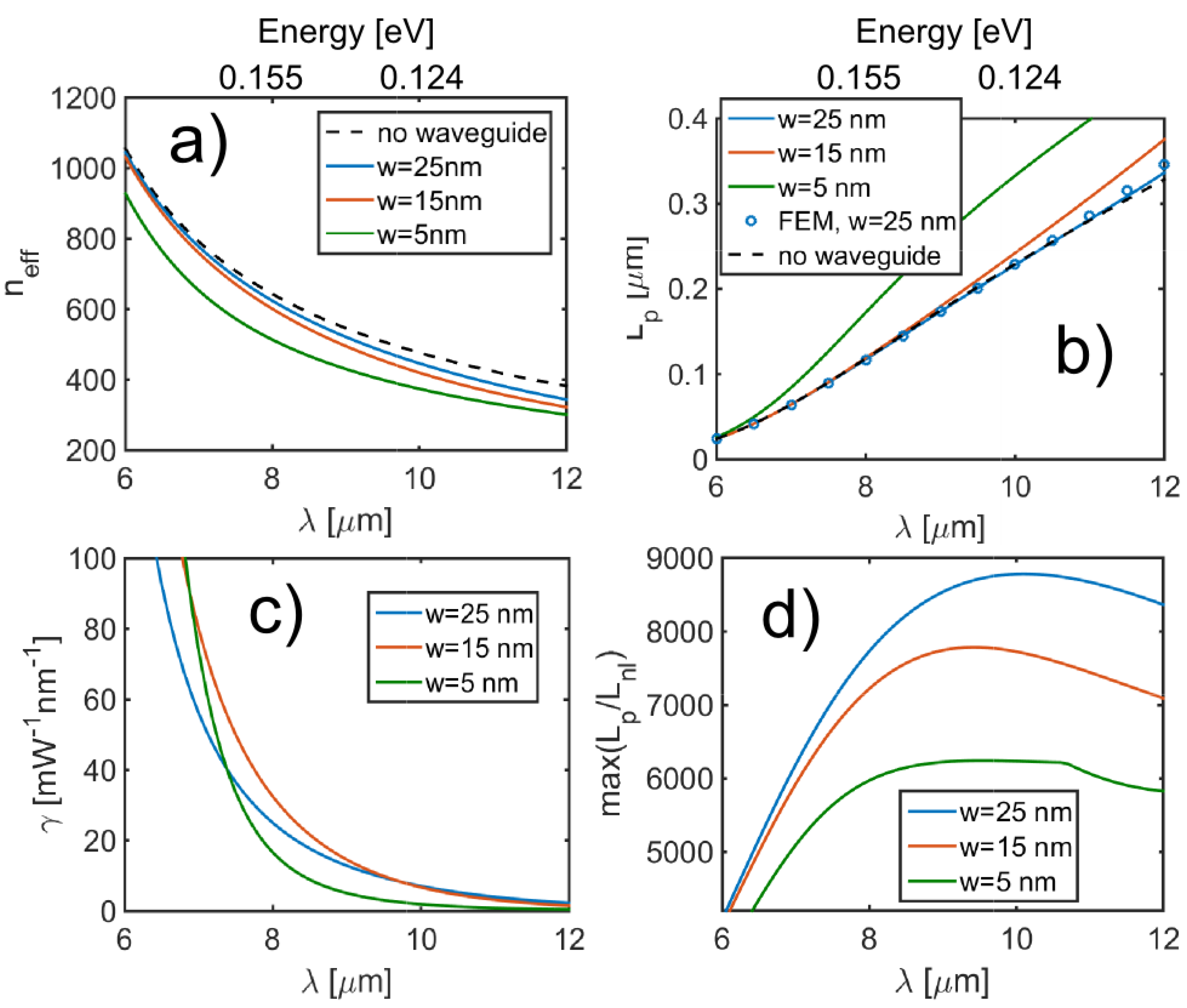
The attenuation length of a localized GSP in a waveguide is generally larger than that of a GSP on a homogeneous graphene sheet, and it grows as the waveguide width w decreases [17]. This tendency is due to GSP de-localization in narrow waveguides. However, typical propagation distances dictated by the damping still remain relatively short, well below 1 μm. To observe any nonlinear effects over such short distances, one needs to have the characteristic nonlinear length $L_{nl}=1/\left(\gamma P\right)$ to be considerably shorter than $L_p$. While the nonlinear length is inversely proportional to input power P, the important characteristic of a waveguide is the critical power, for which local field intensities are still below the damage threshold of graphene and dielectrics involved. Setting the threshold intensity to $I_d={10}^{14}$ $W/m^2$[37], the minimal nonlinear distance is found to be several orders of magnitude below the attenuation length over the broad wavelength range in mid-infrared, see Figure 2d. In particular, for the waveguide of width w = 25 nm the optimal wavelength is identified at around λ = 10 μm, where $\max (L_{nl}/L_P)\approx 9000$ and the maximal efficiency of nonlinear processes is expected.

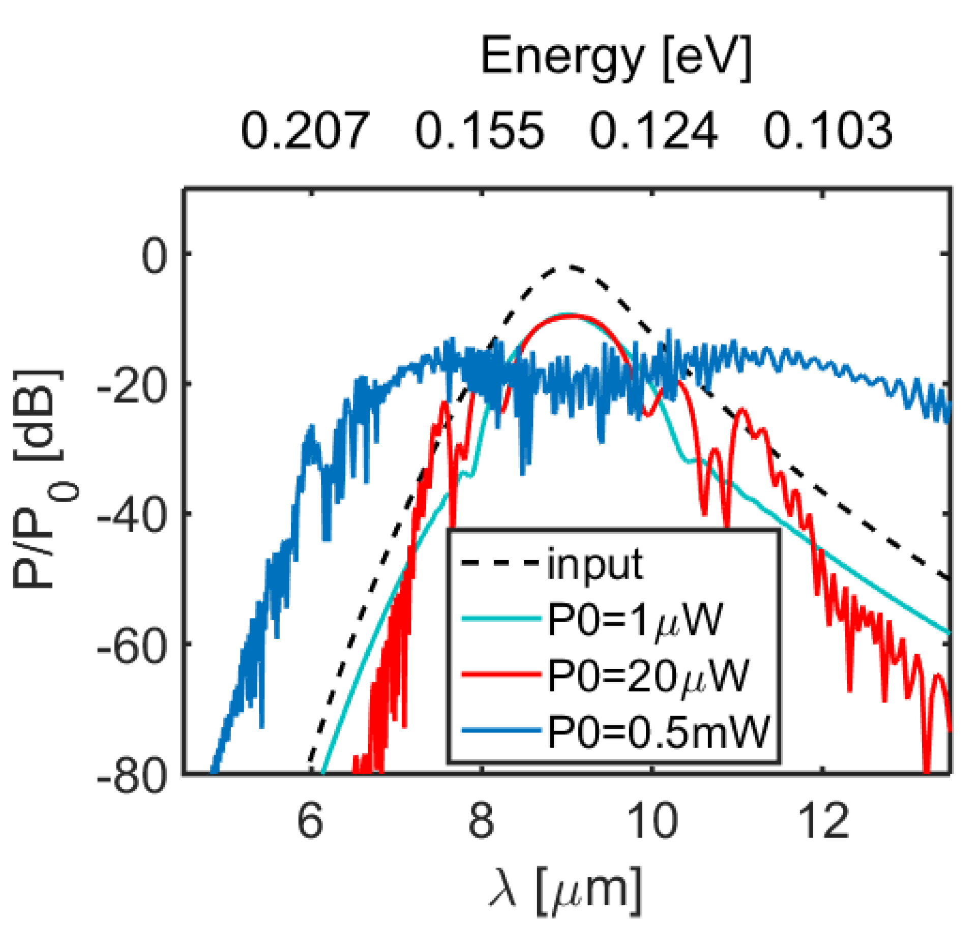
Figure 3. Numerically computed output spectra for propagation of a 100 fs sech pulse with the peak power $P_0$ in the 25 nm wide and 150 nm long GSP wavegide.

Figure 3. Numerically computed output spectra for propagation of a 100 fs sech pulse with the peak power $P_0$ in the 25 nm wide and 150 nm long GSP wavegide.

To illustrate the nonlinear functionality of GSP waveguides, here we consider the spectral broadening process of a short pulse propagating in a 25 nm wide waveguide. We set the initial pulse to be $T_0=100$ fs long (FWHM, sech pulse), centered at ${\lambda }_0$ = 9 μm and with a variable peak power $P_0$. The nonlinear coefficient at this wavelength is $\gamma \approx 1.3$×${10}^{13}$W${}^{-1}{m}^{-1}$, and the critical power is $P_{cr}\approx 4$ mW, cf. also bottom panel if Figure 1. The attenuation constant is $\alpha \approx 5.6$$\mu m^{-1}$, which gives the attenuation length $L_p\approx 180$ nm. The waveguide length was set to $L=150$ nm. The dispersion at ${\lambda }_0$ = 9 μm is computed as ${\beta }_2={\partial }^2\beta /\partial {\omega }^2=$ 9.2 × 10${}^{-21}$s${}^2/m$. For the chosen pulse duration, this gives the dispersion length $L_d=T_0^2/{\beta }_2\approx$ 1.1 μm [35]. Hence the dispersive spreading of the pulse is practically negligible over the full waveguide length, which helps to sustain high efficiency of the nonlinear spectral broadening. In Figure 3 output spectra for different input peak powers are plotted. For the peak power as low as 0.5 mW a considerable spectral broadening can be observed. The generated mid-infrared supercontinuum covers more than one optical octave and spans from λ = 6 μm to λ > 13 μm. While this peak power is well below the estimated critical power $P_{cr}$, a similar spectral broadening could be observed in samples with shorter attenuation lengths, e.g., due to reduced relaxation times τ in graphene, by increasing $P_0$ further.

4. Summary

We introduce a comprehensive set of analytical and numerical tools for the description of pulse propagation and frequency conversion processes in GSP waveguides of arbitrary geometry. The generic propagation Equation (28) and its simplified version (36), together with the nonlinear and damping coefficients due to graphene conductivity are derived following perturbation expansion of Maxwell equations with graphene being treated as the nonlinear boundary condition. Unlike the conventional and widely used models, originally derived for bulk materials [35], our approach does not require introduction of an artificial graphene thickness, and thus does not suffer from any related errors.

As an example, we considered GSP waveguides formed by a local modification of Fermi energy. Remarkably, such waveguides are found to be an outstanding platform for nonlinear functional and extremely compact plasmonic circuits in the mid-infrared to terahertz range. In particular, a supercontinuum generation covering more than one optical octave from a 100 fs input pulse with the peak power as low as $0.5$ mW is demonstrated in a compact 25 nm wide and 150 nm long waveguide. The compactness of the waveguide and the low powers of operation could play the decisive role for future development of on-chip integrated light sources in the spectral range, which is of high importance for many applications in spectroscopy, chemical and bio-sensing, medical imaging.

References

- Maier, S.A. Plasmonics: Fundamentals and Applications; Springer: New York, NY, USA, 2007. [Google Scholar]
- Barnes, W.L.; Dereux, A.; Ebbesen, T.W. Surface plasmon subwavelength optics. Nature 2003, 424, 824–830. [Google Scholar] [CrossRef] [PubMed]
- Ebbesen, T.W.; Genet, C.; Bozhevolnyi, S.I. Surface-plasmon circuitry. Phys. Today 2008, 61, 44–50. [Google Scholar] [CrossRef]
- Sederberg, S.; Elezzabi, A.Y. Coherent visible-light-generation enhancement in silicon-based nanoplasmonic waveguides via third-harmonic conversion. Phys. Rev. Lett. 2015, 114. [Google Scholar] [CrossRef]
- Milian, C.; Skryabin, D.V. Nonlinear switching in arrays of semiconductor on metal photonic wires. Appl. Phys. Lett. 2011, 98. [Google Scholar] [CrossRef]
- Grigorenko, A.N.; Polini, M.; Novoselov, K.S. Graphene plasmonics. Nat. Photon. 2012, 6, 749–758. [Google Scholar] [CrossRef]
- Low, T.; Avouris, P. Graphene plasmonics for terahertz to mid-infrared applications. ACS Nano 2014, 8, 1086–1101. [Google Scholar] [CrossRef] [PubMed]
- Jablan, M.; Buljan, H.; Soljacic, M. Plasmonics in graphene at infrared frequencies. Phys. Rev. B 2009, 80. [Google Scholar] [CrossRef]
- Yan, H.; Low, T.; Zhu, W.; Wu, Y.; Freitag, M.; Li, X.; Guinea, F.; Avouris, P.; Xia, F. Damping pathways of mid-infrared plasmons in graphene nanostructures. Nat. Photon. 2013, 7, 394–399. [Google Scholar] [CrossRef]
- Nikitin, A.Y.; Guinea, F.; García-Vidal, F.J.; Martín-Moreno, L. Edge and waveguide terahertz surface plasmon modes in graphene microribbons. Phys. Rev. B 2011, 84. [Google Scholar] [CrossRef]
- Zhu, X.; Yan, W.; Mortensen, N.A.; Xiao, S. Bends and splitters in graphene nanoribbon waveguides. Optics 2013, 21, 3486–3491. [Google Scholar] [CrossRef] [PubMed]
- Christensen, J.; Manjavacas, A.; Thongrattanasiri, S.; Koppens, F.H.L.; de Abajo, F.J.G. Graphene plasmon waveguiding and hybridization in individual and paired nanoribbons. ACS Nano 2012, 6, 431–440. [Google Scholar] [CrossRef] [PubMed]
- Forati, E.; Hanson, G.W. Surface plasmon polaritons on soft-boundary graphene nanoribbons and their application in switching/demultiplexing. Appl. Phys. Lett. 2013, 103. [Google Scholar] [CrossRef]
- He, S.; Zhang, X.; He, Y. Graphene nano-ribbon waveguides of record-small mode area and ultra-high effective refractive indices for future VLSI. Opt. Express 2013, 21, 30664–30673. [Google Scholar] [CrossRef] [PubMed]
- Ooi, K.J.A.; Chu, H.S.; Ang, L.K.; Bai, P. Mid-Infrared active graphene nanoribbon plasmonic waveguide devices. J. Opt. Soc. Am. B 2013, 30, 3111–3116. [Google Scholar] [CrossRef]
- Sun, Y.; Zheng, Z.; Cheng, J.; Liu, J. Graphene surface plasmon waveguides incorporating high-index dielectric ridges for single mode transmission. Opt. Commun. 2014, 328, 124–128. [Google Scholar] [CrossRef]
- Zheng, J.; Yu, L.; He, S.; Dai, D. Tunable pattern-free graphene nanoplasmonic waveguides on trenched silicon substrate. Sci. Rep. 2015, 5. [Google Scholar] [CrossRef] [PubMed]
- Lao, J.; Tao, J.; Wang, Q.J.; Huang, X.G. Tunable graphene-based plasmonic waveguides: nano modulators and nano attenuators. Laser Photon. Rev. 2014, 8, 569–574. [Google Scholar] [CrossRef]
- Mikhailov, S.A. Non-linear electromagnetic response of graphene. Eur. Phys. Lett. 2007, 79. [Google Scholar] [CrossRef]
- Mikhailov, S.A.; Ziegler, K. Nonlinear electromagnetic response of graphene: Frequency multiplication and the self-consistent-field effects. J. Phys. Condensed Matter 2008, 20. [Google Scholar] [CrossRef] [PubMed]
- Glazov, M.; Ganichev, S. High frequency electric field induced nonlinear effects in graphene. Phys. Rep. 2014, 535, 101–138. [Google Scholar] [CrossRef]
- Hendry, E.; Hale, P.J.; Moger, J.; Savchenko, A.K.; Mikhailov, S.A. Coherent Nonlinear Optical Response of Graphene. Phys. Rev. Lett. 2010, 105. [Google Scholar] [CrossRef]
- Chu, S.; Wang, S.; Gong, Q. Ultrafast third-order nonlinear optical properties of graphene in aqueous solution and polyvinyl alcohol film. Chem. Phys. Lett. 2012, 523, 104–106. [Google Scholar] [CrossRef]
- Zhang, H.; Virally, S.; Bao, Q.; Kian Ping, L.; Massar, S.; Godbout, N.; Kockaert, P. Z-scan measurement of the nonlinear refractive index of graphene. Opt. Lett. 2012, 37, 1856–1858. [Google Scholar] [CrossRef] [PubMed]
- Gu, T.; Petrone, N.; McMillan, J.F.; van der Zande, A.; Yu, M.; Lo, G.Q.; Kwong, D.L.; Hone, J.; Wong, C.W. Regenerative oscillation and four-wave mixing in graphene optoelectronics. Nat. Photon. 2012, 6, 554–559. [Google Scholar] [CrossRef]
- Hong, S.Y.; Dadap, J.I.; Petrone, N.; Yeh, P.C.; Hone, J.; Osgood, R.M. Optical third-harmonic generation in graphene. Phys. Rev. X 2013, 3. [Google Scholar] [CrossRef]
- Kumar, N.; Kumar, J.; Gerstenkorn, C.; Wang, R.; Chiu, H.Y.; Smirl, A.L.; Zhao, H. Third harmonic generation in graphene and few-layer graphite films. Phys. Rev. B 2013, 87. [Google Scholar] [CrossRef]
- Rao, S.M.; Lyons, A.; Roger, T.; Clerici, M.; Zheludev, N.I.; Faccio, D. Two-dimensional materials and the coherent control of nonlinear optical interactions. 2015; arXiv:1503.07665. [Google Scholar]
- Gorbach, A.V. Nonlinear graphene plasmonics: Amplitude equation for surface plasmons. Phys. Rev. A 2013, 87. [Google Scholar] [CrossRef] [Green Version]
- Smirnova, D.A.; Gorbach, A.V.; Iorsh, I.V.; Shadrivov, I.V.; Kivshar, Y.S. Nonlinear switching with a graphene coupler. Phys. Rev. B 2013, 88. [Google Scholar] [CrossRef] [Green Version]
- Gorbach, A.V.; Marini, A.; Skryabin, D.V. Graphene-clad tapered fiber: effective nonlinearity and propagation losses. Opt. Lett. 2013, 38, 5244–5247. [Google Scholar] [CrossRef] [PubMed]
- Mikhailov, S.A. Quantum theory of the third-order nonlinear electrodynamic effects of graphene. 2015; arXiv:1506.00534. [Google Scholar]
- Sukhorukov, A.A.; Solntsev, A.S.; Kruk, S.S.; Neshev, D.N.; Kivshar, Y.S. Nonlinear coupled-mode theory for periodic plasmonic waveguides and metamaterials with loss and gain. Opt. Lett. 2014, 39, 462–465. [Google Scholar] [CrossRef] [PubMed]
- Zhao, X.; Gorbach, A.V.; Skryabin, D.V. Dispersion of nonlinearity in subwavelength waveguides: derivation of pulse propagation equation and frequency conversion effects. J. Opt. Soc. Am. B 2013, 30, 812–820. [Google Scholar] [CrossRef]
- Agrawal, G.P. Nonlinear Fiber Optics, 5th ed.; Academic Press: Boston, MA, USA, 2013. [Google Scholar]
- Falkovsky, L.A. Optical properties of graphene. J. Phys. Conf. Ser. 2008, 129. [Google Scholar] [CrossRef]
- Roberts, A.; Cormode, D.; Reynolds, C.; Newhouse-Illige, T.; LeRoy, B.J.; Sandhu, A.S. Response of graphene to femtosecond high-intensity laser irradiation. Appl. Phys. Lett. 2011, 99. [Google Scholar] [CrossRef]
© 2015 by the authors; licensee MDPI, Basel, Switzerland. This article is an open access article distributed under the terms and conditions of the Creative Commons Attribution license (http://creativecommons.org/licenses/by/4.0/).
Share and Cite
MDPI and ACS Style
Gorbach, A.V. Graphene Plasmonic Waveguides for Mid-Infrared Supercontinuum Generation on a Chip. Photonics 2015, 2, 825-837. https://doi.org/10.3390/photonics2030825
AMA Style
Gorbach AV. Graphene Plasmonic Waveguides for Mid-Infrared Supercontinuum Generation on a Chip. Photonics. 2015; 2(3):825-837. https://doi.org/10.3390/photonics2030825
Chicago/Turabian StyleGorbach, Andrey V. 2015. "Graphene Plasmonic Waveguides for Mid-Infrared Supercontinuum Generation on a Chip" Photonics 2, no. 3: 825-837. https://doi.org/10.3390/photonics2030825