1. Introduction
In recent years, the use of numerical methods has become very common in modeling the flow around marine propellers. Although the experimental methods have a higher accuracy and reliability than numerical methods, the higher costs and the need for special equipment has caused numerical methods to be preferred.
The boundary element method (BEM) is one of the methods used to solve the governing equations of fluid mechanics, acoustics, electromagnetics, etc. In this method, using mathematical theorems, the equations from the interior of the solution domain are transferred to the boundaries of the domain. Therefore, compared to other numerical methods such as finite element or finite volume method which interior of domain should be considered, BEM exhibits less solution time and computation cost and therefore it is preferred to other methods.
The panel method is one of boundary element methods. In this method, the surface of the body is divided into small panels and a combination of source and doublets is distributed to each panel. After calculating the strength of sources and doublets, velocity and pressure distribution on surface panels can be obtained. For lifting bodies, a wake surface should be assumed at the trailing edge of body, and the effect of panels of this surface on body panels should be considered.
In recent decades, the panel method has been widely used to solve the flow around the bodies, especially marine propellers. A literature review shows that a lot of research has been done on the use of the panel method for the hydrodynamic analysis of objects. For instance, Hess and Smith [
1], in 1962, invented the panel method for analyzing the motion of three dimensional bodies in fluid. The formulation of these researchers was presented for the arbitrary three dimensional bodies and could not be used for lifting bodies. In 1972, Hess [
2] developed this method for lifting bodies and calculated the pressure distribution around an aircraft model and lift force. The panel method was first used in 1985 by Hess and Valarezo [
3] to model the flow around the ship propeller. In this study, they obtained the pressure distribution around a propeller using quadrilateral panels and calculated the thrust and torque coefficients. In 2010, Baltazar et al. [
4] modeled cavitation around a propeller using the panel method. The results of this study show that the panel method can model cavitation on propeller blades with good accuracy. Also, several papers have been published between the years 1985 to 2010, but most have done similar work.
In 2010, Gaggero et al. [
5] modeled the flow around the propeller using the panel method and computational fluid dynamics. The results of the panel method show that this method has a good and acceptable accuracy compared to the CFD method.
According to the importance of propeller noise, various methods have been proposed to reduce it. Methods used to reduce the noise of marine propellers can be divided into two main methods, namely:
- -
Using equipment
- -
Modification of the geometry
Each of these methods is fully described in a review paper published by Ebrahimi et al. [
6]. In recent years, calculating the noise of marine propellers using numerical methods has also been developed by researchers. For numerical calculation of noise, a numerical method such as panel method is required to obtain flow quantities and then these quantities are used as input for calculation of noise for a receiver at the desired location. Seol and Park [
7] carried out several experiments on a propeller model in MOERI cavitation tunnel and measured the noise of propeller in cavitating and non-cavitating condition. Also, they used combination of time domain acoustic analogy and panel method for the numerical investigation of the propeller noise.
In another study by Kellett et al. [
8] in 2013, the noise generated by the propeller of a LNG carrier ship was measured numerically and experimentally. Bagheri et al. [
9] conducted a research on a three bladed propeller of the Gawn series and used the ANSYS Fluent commercial software for calculation of the propeller noise. Testa et al. [
10] calculated the noise of E779A propeller model by using the FW-H equations in presence of unsteady sheet cavitation. They also used potential-based panel method for modelling flow around propeller. Gorji et al. [
11] performed a research on calculation of noise of a marine propeller using a RANS solver in the low frequencies band.
Bagheri et al. [
12] carried out some numerical and experimental tests on the noise of marine propellers and the effects of cavitation on the sound pressure level of propeller. They used viscous flow with FW-H solver for noise calculation.
In present research, a boundary element method is used for hydrodynamic analysis of marine propellers. Also, the FW-H equations are used for acoustic performance analysis of these propellers. For this purpose, two codes have been developed by authors and their results validated using experimental tests carried out in cavitation tunnel of Sharif University of Technology. The most significant novelty of our paper is that we used experimental noise measurements to validate the results of the FW-H equations code.
2. Formulation of the Panel Method
For development of the panel method formulation for marine propeller, the flow around propeller in computational domain of
is assumed to be irrotational, incompressible and inviscid. By these assumptions, the flow governing equations (Navier-Stokes equation) are simplified into the three-dimensional Laplace equation where is
. By using Green’s second identity, the general solution of this equation is as follows [
13]:
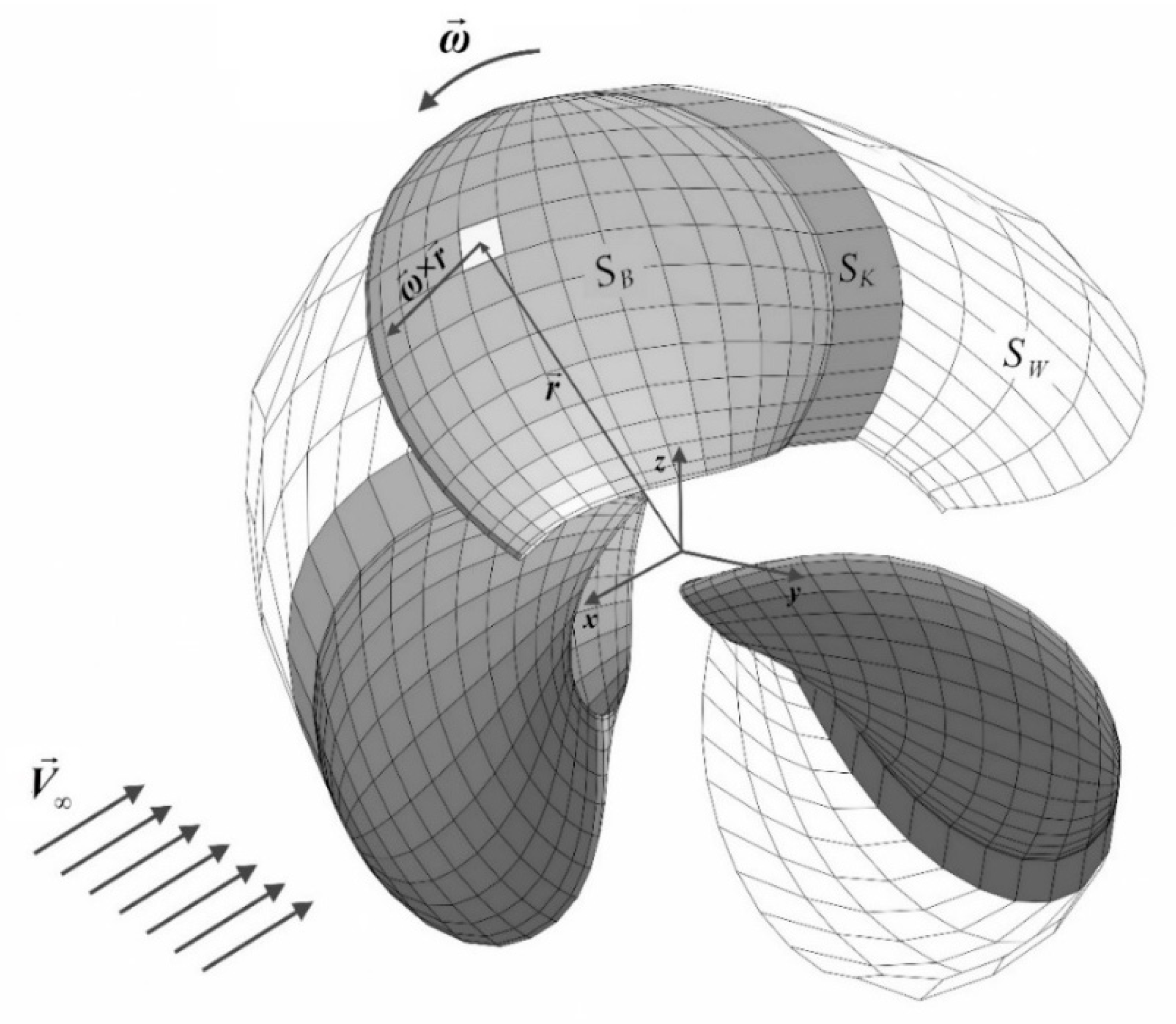
On the right-hand side of the Equation (1), integrating is done on the surface
S, which includes the body surface, Kutta strip and wake surfaces of the object (
Figure 1). If the points
P,
Q and
O are defined as the control point, source point and the origin of the coordinates, respectively, the distance vector
is defined as follows:
Now, if we suppose
and
, where
is potential of flow, Equation (1) becomes:
In the case where
P is outside of the domain
, then
and
satisfy Laplace’s equation [
13]. Therefore, the first and second terms on the left-hand side of Equation (3) will be zero. Then:
In the case of flow around the propeller, the point
P is located on the body surface. When point
P approaches to point
Q and
, the above integral is singular
. Therefore, the point
P should be excluded from
S using a small hemisphere of radius
. Therefore, the integration region will change to
:
Using mathematical methods, the value of second integral is
. Then Equation (5) becomes:
This equation gives the potential of flow
at any point of body surface in terms of
and
on the boundaries of domain. In Equation (6), the first and second terms of the integral can be interpreted as a dipole with strength of
and a source with strength of
, respectively. To expand the above equation, as shown in
Figure 1, the integration surface
S is divided to body surface
, Kutta strip
, and wake surface
. Also,
and
are number of panels on body surface, Kutta strip, and wake surface, respectively.
Therefore, Equation (6) can written as below:
The thickness of Kutta and wake surfaces are assumed to be zero. Then,
for these surfaces becomes zero. So:
This formulation is equivalent to distributing a source with strength of
on each panel of the body surface and a doublet with strength of
on each panel of the body surface, Kutta strip and wake surface. For greater simplicity, the strength of doublets on the Kutta strip and wake surface are displayed by
. The final form of Equation (8) is as follows:
2.1. Boundary Conditions
Applying boundary conditions is one of the most important steps in solving problems by numerical methods. The first boundary condition that is applied is the non-entrance condition. If the propeller assumed to be rigid, the fluid particles cannot enter into the surface and the normal velocity will be zero on the surface of the propeller. If the propeller is operating in a uniform axial flow with velocity of
and rotates with angular velocity of
, as shown in
Figure 1, the total velocity of point
A on propeller blade is:
Then, the non-entrance condition for all panels of body surface is [
14]:
Then, Equation (9) becomes:
We can rewrite the above equation in series form as follows:
where the points
P and
Q are assumed to be the center of panel
i and
j, respectively.
Aij and
Bij are known as influence coefficients and can be calculated according to Delhommeau [
15]. The first and second terms in right-hand side of Equation (13) are obtained from non-entrance boundary condition and from previous time step, respectively. Therefore, the unknowns of the above equation are the strength of doublets on body panels and doublets on Kutta strip, hence
unknowns. Another boundary condition that is used to solve this problem is the Kutta condition. This condition for lifting bodies states that the flow should leave trailing edge smoothly and the velocity of flow there be finite [
13]. One of the best ways to apply this condition is presented by Morino [
16]:
This means that strength of Kutta strip doublets is equal to difference of strength of upper and lower doublets. Equation (13) will give equations and equations will be added to system of equations by applying Kutta condition. Finally, by solving this set of equations, all unknowns will be obtained.
2.2. Hydrodynamic Forces
After the calculation of velocity potential, the total velocity on each panel can be calculated using numerical differentiation methods. Then, the unsteady Bernoulli’s equation was used for calculation of total pressure [
17]:
where
and
denote the surface gradient and time derivate of velocity potential. Propeller thrust can be calculated by integration of pressure forces on panels of propeller surface. Also, viscous forces should be obtained by using empirical formulas for surface friction coefficient
of each panel [
18]:
where
is local Reynolds number based on radial location of panel
and is
. The viscous drag of each panel is calculated as below [
17]:
where
and
. Also,
is blade surface perturbation velocity and can be obtained by taking surface gradient of velocity potential on blade panels. Then, total force and torque of propeller are obtained as [
19]:
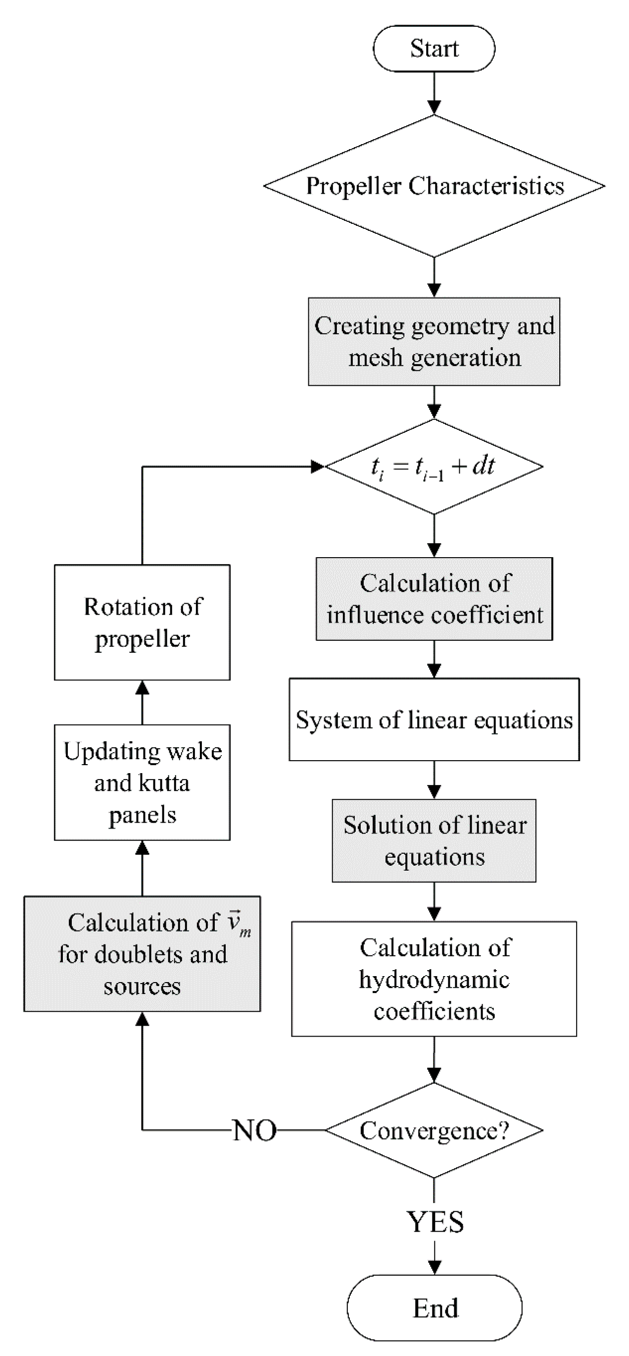
Flowchart of panel method for calculation of hydrodynamic coefficient of propeller is shown in
Figure 2. Initially, geometry of propeller and panels are generated by a function. A Kutta strip is also created due to geometric considerations, propeller rotation and flow velocity. In the next step, a function calculates the influence coefficients for the sources and doublets. Then, the systems of linear equations of Equation (13) is formed and then solved using iterative methods. By solving the equations, the velocity potential is obtained on the panels of body surface. With numerical derivation of potentials, velocity and pressure and on each panel are calculated and hydrodynamic coefficients of propeller are obtained. This process repeated until the solution converges. In this flowchart,
is the mean perturbation velocity of the points located on wake and Kutta surface. If these points are located in
position in time t, new position
of points in time
t + dt can be obtained using the following equation:
where
is calculated as below [
19]:
3. Validation of Results of Panel Method
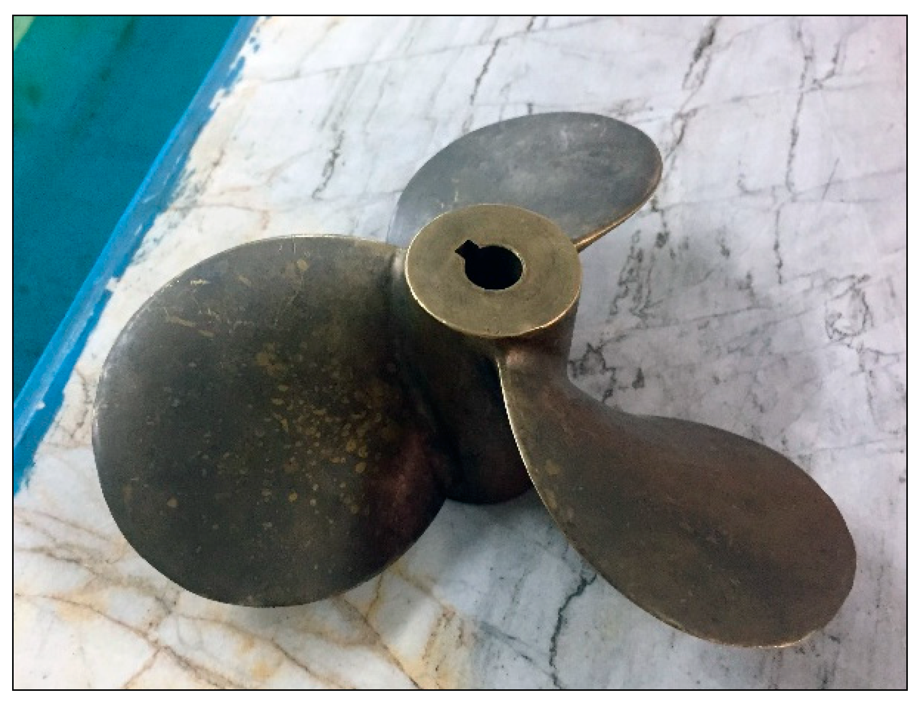
One of the most common propellers that has been used for the validation of numerical methods is the DTMB 4119 propeller. This propeller is shown in
Figure 3. Also, the main particulars and details of geometry are given in
Table 1 and
Table 2, respectively.
P is propeller pitch, r is radius of each section, R is propeller radius, c is chord of each section, D is propeller diameter, t
max is Maximum thickness of each section and f
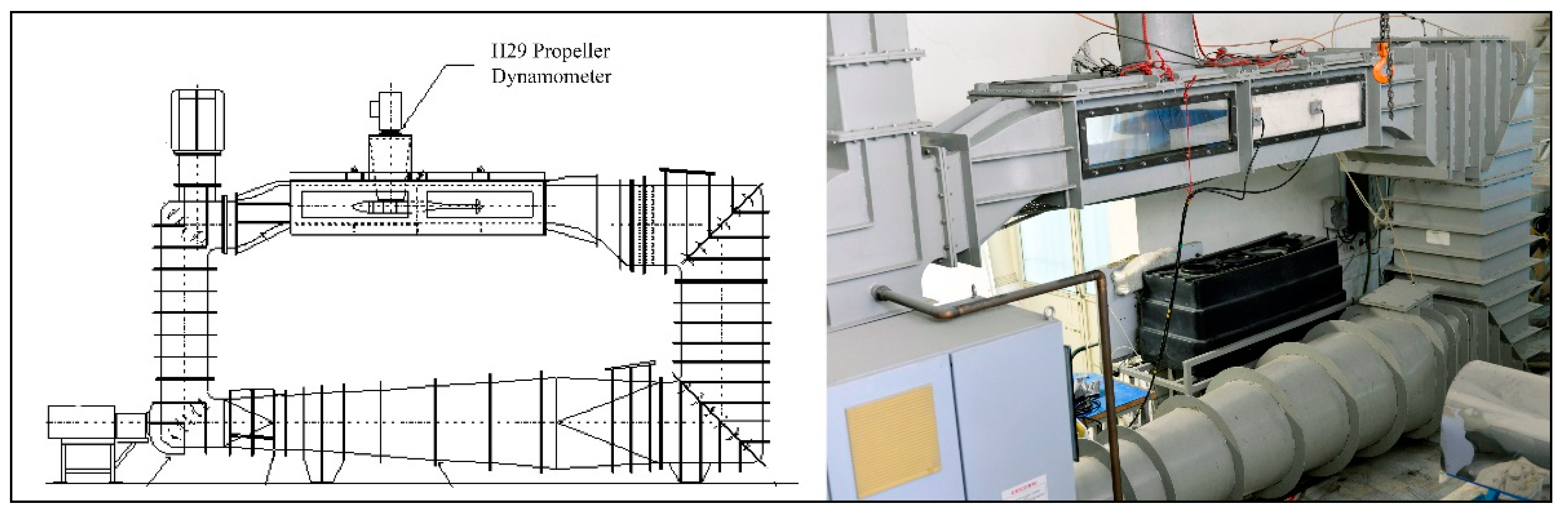
max is maximum camber. For the validation of the results of numerical modeling for hydrodynamics and noise of DTMB 4119 propeller, some experiments were carried out with a model propeller in a cavitation tunnel of the Marine Engineering Laboratory of Sharif University of Technology (
Figure 4). For measuring the thrust and torque of propeller model, a H29 dynamometer has been used in this tunnel.
The developed code can also create the geometry of the propeller and generate mesh for it. For this purpose, the profile of propeller blades, the number of blades, the rake and skew angle and the desired grid size should be specified as input. In the panel method, it is not common to specify mesh dimensions. Because of the cosine spacing of panels in chordwise and spanwise directions, the exact size of panels cannot be specified. Grid size is shown as
m ×
n which
m and
n are number of elements in chordwise and spanwise, respectively. For optimization of the grid size, thrust coefficient for design advance ratio (
J = 0.833) is calculated for some different grids, and error of numerical results compared with experimental results for each grid size are presented in
Table 3 and
Figure 5. All simulations are carried out using Intel Core i7 2.6 GHz and 8 GB of RAM. Also, the CPU times for the panel method are given in
Table 3.
It can be seen from
Figure 5 that the grid size of
compared to other grids has more appropriate CPU time and error, and then the grid is used to simulate propeller. After simulation of flow around DTMB 4119 propeller, wake surface and hydrodynamic coefficients of propeller (Thrust, torque and efficiency) are obtained. In
Figure 6, the wake surface of the propeller is shown for different advance ratios.
As shown in
Figure 6, in low advance ratios which ship speed is low and propeller load is high (heavy duty conditions of propeller), disks of wake surface are closer together and wake rollup is intense but in higher advance ratios, disks of wake surface are more spacious and rollup is very low. Numerical simulation of propeller is performed by developed code for various advance ratios and
Figure 7 compares the hydrodynamic coefficients of the propeller obtained by the panel method with experimental data.
The pressure distribution in the advance ratio of
for different radial sections of the propeller blade is compared with experimental measurements [
21] in
Figure 8.
According to
Figure 7, there is satisfactory agreement between the hydrodynamic coefficients obtained from the panel method and experimental results. The maximum error of the trust coefficient calculated by the panel method is about 4% and for torque coefficient is about 7%. As can be seen in
Figure 8, pressure distribution obtained from the panel method is in good agreement with the experimental data. This shows that the accuracy of the panel method results is acceptable. One reason for the greater error of the torque coefficient is the use of empirical formulas in the calculation of the friction resistance of each panel. According to the above results, the panel method can be used for hydrodynamic performance analysis of marine propellers.
4. Acoustic Formulations
In most acoustic problems, rigid bodies located in the fluid flow have very important effects on the generated noise. For this reason, Williams and Hawkings [
22] in 1969 developed the Lighthill equations [
23] with the assumption of rigid bodies. The equations presented by these researchers in acoustic science are known as the FW-H model. For solving the FW-H equation, Farassat et al. [
24] presented a method that can predict the generated noise of moving object with arbitrary geometry. According to this formulation, total sound pressure can
expressed as below [
24]:
where
and
denote the thickness and loading pressure, respectively. Thickness pressure is due to the fluid displacement caused by movement of the body within the fluid and classified as monopole noise source. Another phenomenon caused by the motion of the non-symmetric body in fluid is the distribution of positive and negative pressure on the face and back of the body. In fact, this pressure distribution is the main source of trust force in propellers. Pressure difference on both sides of the body create a dipole noise source which is referred as loading pressure. This solution is obtained with assumption of low Mach number, and hence the quadrupole noise can be neglected. These components are calculated through the following relations [
24]:
where
ρ is fluid density in
,
c is sound speed in
,
is the noise source velocity in
,
is distance vector from noise source to receiver in
,
is magnitude of
in
, Mach number is
,
is pressure force in
and
is hydrodynamic pressure in
. The dot over variables means time derivate of the variable. The
subscript in this equation means that the calculations must be done using values at the retarded time.
In the first step of noise calculation, the flow around the body is simulated using the panel method and flow quantities such as pressure and velocity are obtained for panels on the body surface. Then, for receiver in position of
and time of
ti, retarded time
is obtained for panel
j. After this step, all quantities required in Equation (20) must be calculated for each panel at the retarded time, numerical integrals of the equation are solved for each panel, and the acoustic pressure of each element is obtained. By summing up the acoustic pressures of all the elements, a total acoustic pressure is obtained for the specified receiver. Flowchart of noise calculation using FW-H equations is shown in
Figure 9.
5. Noise of DTMB 4119 Propeller
The noise generated by the propeller is one of the most important components of the vessels noise [
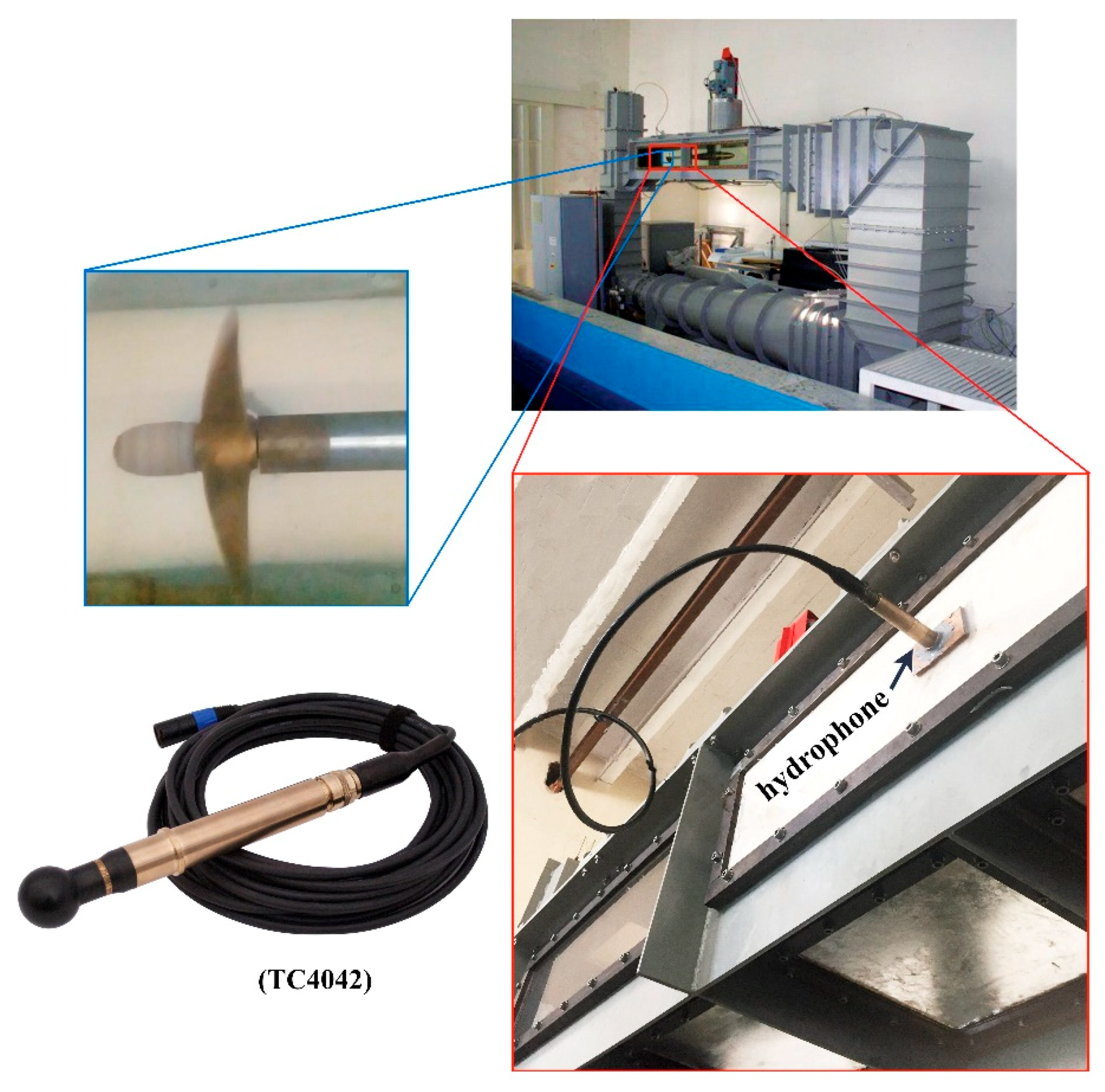
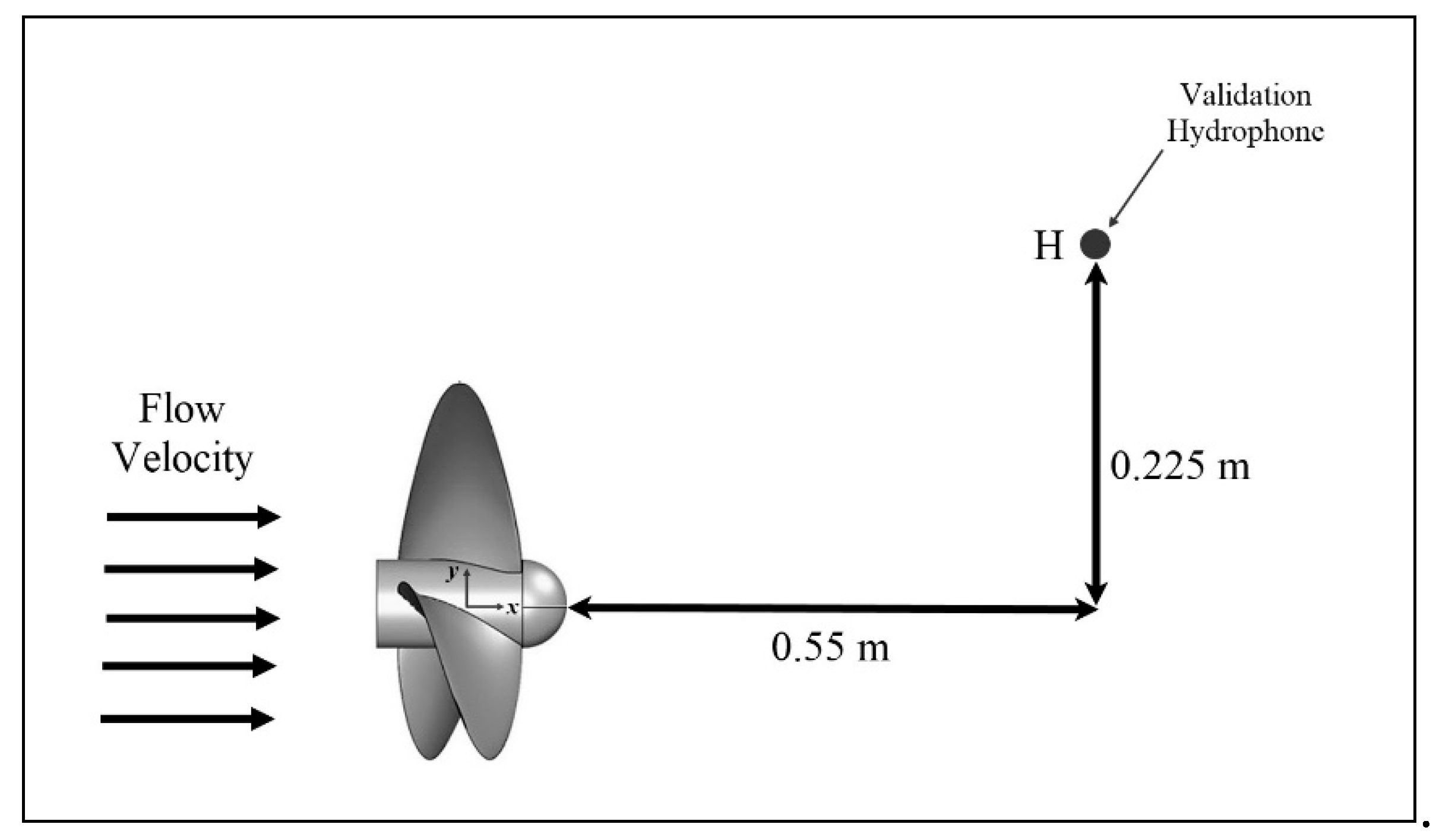
6]. Therefore, measuring and calculating the propeller noise is one of the interesting research subjects in naval engineering. In the first step, the results of the developed FW-H code for noise calculation should validated using experimental results obtained in cavitation tunnel. For measuring the noise of propeller, a TC4042 hydrophone has been used in cavitation tunnel of Sharif University of Technology. The arrangement of this validation hydrophone is shown in
Figure 10. Also, the location of this hydrophone is given in
Figure 11.
For validation of results of FW-H code, noise measurements done in cavitation tunnel under below conditions:
- -
Flow velocity: 2.2 m/s
- -
Propeller RPM: 792
- -
Advance ratio (J): 0.833
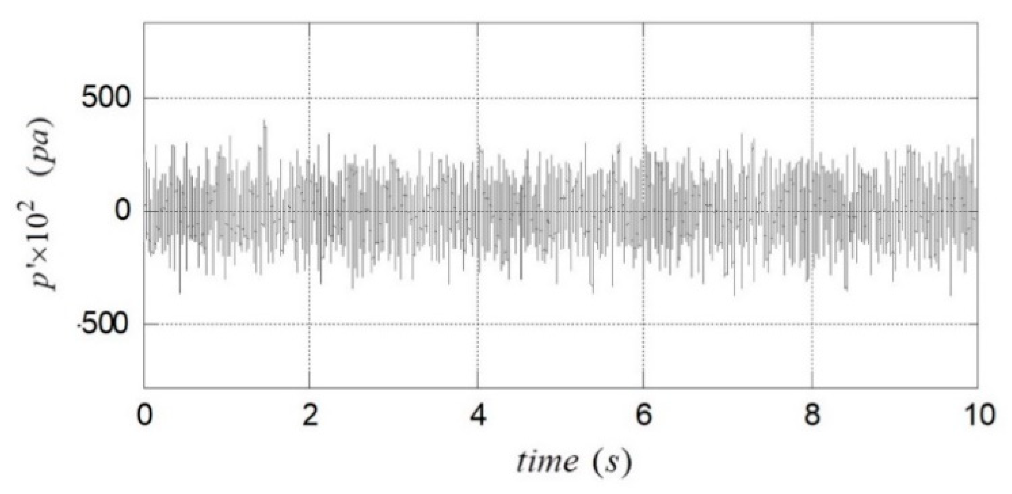
The time history of acoustic pressure as measured by validation hydrophone is shown in
Figure 12.
In the post-processing stage, acoustic pressure from time domain in transferred to frequency domain by using the fast Fourier transform (FFT) and the sound pressure level is calculated using the following formula [
25]:
where
is the reference pressure and related to threshold of a normal human hearing for frequency of 1 kHz which for water is
[
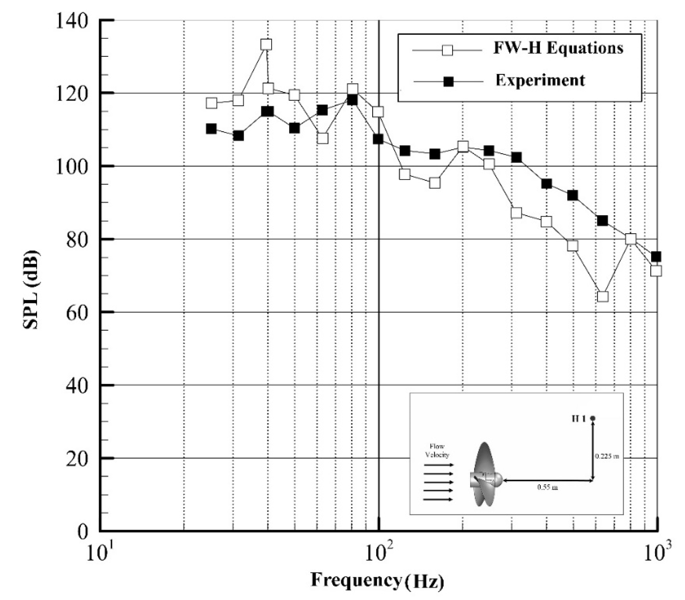
26]. The numerical results of noise obtained by own developed code compared by experimental results in
Figure 13. Propeller and flow conditions are the same as the experimental setup.
It can be seen that there is good agreement between the numerical and experimental results of propeller noise, especially in frequencies under 250 Hz. It seems that main sources of error of numerical results are:
- -
Error of panel method code for calculation of pressure and flow velocity: As mentioned in the previous sections, the results of the thrust and torque of the panel method have 4% and 7% error in comparison with the experimental results. Since the FW-H equations use panel method outputs, the above error causes an error in calculating the noise of the impeller.
- -
The error of FW-H code for noise calculation: FW-H equations include some integrals that are calculated numerically on the source of noise. Therefore, the numerical calculation error of these equations can cause error in the value of noise. Also, in the solution presented in this study, the quadrupole sources of noise are neglected, which could cause a slight error in the value of propeller noise.
- -
The reflection of sound inside the cavitation tunnel is another reason for the difference between the experimental and numerical results. The restricted space of the cavitation tunnel causes the reverberation of sound emitted by the propeller, which results in an error in the measured noise values. For investigating the effects of sound reverberation on noise data, special equipment is needed which is not available in our laboratory.
Seol et al. [
27] and Yang et al. [
28] carried out some numerical studies on DTMB 4119 propeller, but since the specifications of the propeller used are not the same as the propeller model in our laboratory, the results cannot be compared.
By looking more precisely into results, it founds that both experimental and numerical results have peaks in some frequencies. It seems that these are Blade Passing Frequencies (
BPF) of propeller. For the propeller, the rate at which the blades pass by a fixed position is called the
BPF. This frequency is known as the blade passing frequency (
BPF) of the blade. As regards the propeller, the
BPF and its higher harmonics can be calculated as:
where
Z is number of propeller blades,
rps is the frequency of propeller rotation in Hz and
h is no of harmonic. When receiver is located in an asymmetric location relative to blades, the noise of propeller in BPFs will have local peaks in comparison to other frequencies. For the receiver, which is located in the hub plane of the propeller, at an equal and constant distance from the blades at all times,
BPF could not be seen in the SPL diagram. For noise diagrams in
Figure 13,
rps is 13.2 and
Z is 3. Therefore, BPF for three first harmonics of propeller is about 39.6, 79.2 and 118.8 Hz and noise results have peaks in the first two frequencies.
After the validation of FW-H code, propeller noise calculations were made for four hydrophones (receivers). Two hydrophones located in the propeller rotation plane and two hydrophones located in front of propeller hub. The location of hydrophones and their coordinates are given in
Figure 14 and
Table 4.
The noise of the propeller as calculated by the FW-H code for hydrophones H1 and H2 are presented in
Figure 15. Noise predictions were made at a flow speed of 2.2 m/s and RPM of 792 where
J = 0.833.
Results shown in
Figure 15 reveals that by increasing the distance of hydrophone from propeller, noise of H2 decreased significantly in comparison with H1. Also, in
Figure 16, the propeller noise in hydrophones H3 and H4 are presented.
As can be seen in
Figure 16, with an increase of distance from the propeller, noise decreased significantly. Also, in both hydrophones, at a blade passing frequency of 18.22 Hz, the noise has a peak value which is also indicated in the
Figure 16. By comparing
Figure 15 and
Figure 16, it can be seen that the SPL in front of the propeller hub is higher than the SPL in the propeller rotational plane.
6. Conclusions
Measuring and calculating the noise of marine propellers is very important. In this research, the combination of the panel method and FW-H equations has been used to calculate the non-cavitating noise of marine propellers. In the first step, a numerical panel method code is developed to solve the flow around the propeller and calculate the propeller hydrodynamic coefficients. The results of this code in comparison with the experimental results had maximum error of 4% and 7% for thrust and torque coefficients, respectively.
Then, a noise calculation code based on FW-H acoustic equations was developed, which uses the outputs of the panel method code as inputs and calculates the noise of the propeller for the desired receiver. The results of this code are in good agreement with the noise of the propeller obtained using results from a test carried out in cavitation tunnel of Sharif University. Using this code, the propeller noise is measured for four hydrophones with different distances and orientations. With increasing distance from the propeller, the noise of the propeller has been significantly reduced. For the hydrophones located on the rotation plane of the propeller, as predicted by theory and experiments on propeller noise, the maximum noise has occurred at the blade passing frequency. The results show that the SPL in front of the propeller hub is higher than SPL in the propeller rotational plane.
According to the above results, the combination of the panel method and FW-H equations can be used for hydrodynamic and acoustic analysis of marine propellers.


