Memory Efficient Method for Electromagnetic Multi-Region Models Using Scattering Matrices

Abstract

This paper describes the scattering matrix approach to obtain the solution to electromagnetic field quantities in harmonic multi-layer models. Using this approach, the boundary conditions are solved in such way that the maximum size of any matrix used during the computations is independent of the number of regions defined in the problem. As a result, the method is more memory efficient than classical methods used to solve the boundary conditions. Because electromagnetic sources can be located inside the regions of a configuration, the scattering matrix formulation is developed to incorporate these sources into the solving process. The method is applied to a 3D electromagnetic configuration for verification.

1. Introduction

The design and optimization of electrical machines and other electromagnetic applications necessitate accurate models of electromagnetic fields to precisely predict their performance. As these systems and their structures get more complex, it is becoming more difficult to accurately model, e.g., eddy current effects [1,2] or hysteresis effects [3] in both the spatial and time domain. To model electromagnetic field distributions and the related forces and power losses, the finite element method (FEM) is often used because of its ability to produce accurate results when it is correctly utilized. However, the method can be demanding in terms of memory and relatively slow in terms of computation time. Therefore, semi-analytical models have been proposed over the years for increasingly complex structures in both 2D and 3D. One of the semi-analytical models is the harmonic modeling technique [4,5,6,7], which uses a Fourier basis to describe the solutions to the electromagnetic field quantities. By including position dependent material properties, such as the electrical conductivity [8] and the permeability [9,10,11], into the solutions, the spatial distribution of electromagnetic fields can also be accurately modeled for complex devices.

In many electromagnetic configurations, accurate results are obtained using a relatively low number of harmonics. However, for more complex structures, with detailed features compared to the device size, the number of harmonics has to be increased to retain accuracy. Computationally, this leads to an increase in the required memory. In addition, as an electromagnetic configuration has to be divided into regions (or layers), the number of regions influences the required memory. As a result, the number of harmonics that can be considered is limited when a relatively large number of regions has to be incorporated. Consequently, the advantage in terms of memory of the harmonic model in comparison to FEM is reducing. The scattering matrix approach [12,13,14,15,16] reformulates a multiple region electromagnetic problem in such a way that it can be expressed as a single region with in- and out-going fields. Consequently, the dependency of the computational memory on the number of regions is removed. All matrices that are manipulated with this method have a maximum size of $L\times L$, where L is the total number of harmonics. In [12], where the scattering matrices are used to solve a high-frequent electromagnetic problem, the source is an incident wave on one side of the problem. However, to apply the scattering formulation in low-frequent problems in which sources (currents or magnets) are present in regions, the scattering formulation has to be extended to incorporate the related source terms.

In this paper, the scattering matrix approach for harmonic models of electromagnetic configurations is described. Using this approach, the memory required to obtain the solutions of the model is significantly reduced. The method presented in [12] is extended to take electromagnetic sources inside regions into account. The method is verified by application to a 3D electromagnetic configuration presented in [10], where the permeability varies in both periodic directions as a function of position.

2. Model Assumptions

The mathematical models of electromagnetic configurations that can be solved with the method described in this paper are subject to a number of assumptions. The considered models are set up in the Cartesian coordinate system, where, for 2D configurations in one direction, periodicity is assumed. For 3D configurations, two directions are assumed periodic. Because of the periodicity, the solution in the periodic directions is expressed by Fourier series. Based upon the electromagnetic material properties, such as the permeability, permittivity and conductivity, and the electromagnetic field sources, the model is divided into regions in the non-periodic direction. In the non-periodic direction, the properties of a region may not vary, whereas, in the periodic direction, they are allowed to change as a function of position. Lastly, any configuration needs to have an air region at both sides, extending to plus and minus infinity in the non-periodic direction, for the applied method.

3. Scattering Matrix Formulation

For all problems at hand, the Fourier coefficients of describing the electromagnetic fields have the same form. For the remainder of the paper, the non-periodic direction is the z-direction. The z-dependent solution describing the coefficients $\mathbf{u}$ and $\mathbf{v}$ of particular field components of a region i is given by

$$\begin{array}{cc}\hfill {\mathbf{u}}_i& ={\mathbf{Q}}_{\mathbf{u}}i\left(e^{{\mathsf{\lambda }}_{i}z}{\mathbf{c}}_i^{+}+e^{-{\mathsf{\lambda }}_{i}z}{\mathbf{c}}_i^{-}\right)+{\mathbf{p}}_{u,i},\hfill \end{array}$$

(1)

$$\begin{array}{cc}\hfill {\mathbf{v}}_i& ={\mathbf{Q}}_{\mathbf{v}}i\left(e^{{\mathsf{\lambda }}_{i}z}{\mathbf{c}}_i^{+}-e^{-{\mathsf{\lambda }}_{i}z}{\mathbf{c}}_i^{-}\right)+{\mathbf{p}}_{v,i},\hfill \end{array}$$

(2)

where $\mathsf{\lambda }$ is a vector with eigenvalues and ${\mathbf{Q}}_{\mathbf{u}}$ and ${\mathbf{Q}}_{\mathbf{v}}$ are eigenvector matrices. Combined, $\mathsf{\lambda }$ and $\mathbf{Q}$ describe the propagation of field components inside a region. The particular solutions described by ${\mathbf{p}}_u$ and ${\mathbf{p}}_v$ relate source terms, such as coil currents and magnetization, which are known in advance, to the solutions $\mathbf{u}$ and $\mathbf{v}$. All these variables are determined by the properties of a region that is under consideration. The way to obtain these variables for a variety of problems has been described in e.g., [8,9,10]. The unknown coefficients ${\mathbf{c}}_i^{+}$ and ${\mathbf{c}}_i^{-}$ in (1) and (2) are determined by applying continuity boundary conditions between regions.

The continuity boundary conditions force both $\mathbf{u}$ and $\mathbf{v}$ to be continuous on an interface between adjacent regions. Often in harmonic models used for electrical machines, all boundary conditions are gathered in a large matrix which forms a system of linear equations,

$$\begin{array}{c}\hfill \begin{array}{c}\underset{\mathbf{E}}{\underbrace{\left[\begin{array}{cccccccc}{\mathbf{Q}}_{\mathbf{u}}1e^{{\mathsf{\lambda }}_1{h}_1}& {\mathbf{Q}}_{\mathbf{u}}1e^{-{\mathsf{\lambda }}_1{h}_1}& -{\mathbf{Q}}_{\mathbf{u}}2e^{{\mathsf{\lambda }}_2{h}_1}& -{\mathbf{Q}}_{\mathbf{u}}2e^{-{\mathsf{\lambda }}_2{h}_1}& \mathbf{0}& \cdots & \cdots & \cdots \\ {\mathbf{Q}}_{\mathbf{v}}1e^{{\mathsf{\lambda }}_1{h}_1}& -{\mathbf{Q}}_{\mathbf{v}}1e^{-{\mathsf{\lambda }}_1{h}_1}& -{\mathbf{Q}}_{\mathbf{v}}2e^{{\mathsf{\lambda }}_2{h}_1}& {\mathbf{Q}}_{\mathbf{v}}2e^{-{\mathsf{\lambda }}_2{h}_1}& \mathbf{0}& \cdots & \cdots & \cdots \\ \mathbf{0}& \mathbf{0}& {\mathbf{Q}}_{\mathbf{u}}2e^{{\mathsf{\lambda }}_2{h}_2}& {\mathbf{Q}}_{\mathbf{u}}2e^{-{\mathsf{\lambda }}_2{h}_2}& {\mathbf{Q}}_{\mathbf{u}}3e^{{\mathsf{\lambda }}_3{h}_2}& \cdots & \cdots & \cdots \\ ⋮& ⋮& ⋮& ⋮& ⋮& \ddots & ⋮& ⋮\\ \mathbf{0}& \mathbf{0}& \mathbf{0}& \mathbf{0}& \mathbf{0}& \cdots & -{\mathbf{Q}}_{\mathbf{u}}i{e}^{-{\mathsf{\lambda }}_i{h}_{i-1}}& -{\mathbf{Q}}_{\mathbf{u}}i{e}^{{\mathsf{\lambda }}_i{h}_{i-1}}\\ \mathbf{0}& \mathbf{0}& \mathbf{0}& \mathbf{0}& \mathbf{0}& \cdots & -{\mathbf{Q}}_{\mathbf{v}}i{e}^{-{\mathsf{\lambda }}_i{h}_{i-1}}& {\mathbf{Q}}_{\mathbf{v}}i{e}^{{\mathsf{\lambda }}_i{h}_{i-1}}\end{array}\right]}}\left[\begin{array}{c}{\mathbf{c}}_1^{+}\\ {\mathbf{c}}_1^{-}\\ {\mathbf{c}}_2^{+}\\ {\mathbf{c}}_2^{-}\\ {\mathbf{c}}_3^{+}\\ ⋮\\ {\mathbf{c}}_i^{+}\\ {\mathbf{c}}_i^{-}\end{array}\right]=\left[\begin{array}{c}{\mathbf{p}}_{u,2}-{\mathbf{p}}_{u,1}\\ {\mathbf{p}}_{v,2}-{\mathbf{p}}_{v,1}\\ {\mathbf{p}}_{u,3}-{\mathbf{p}}_{u,2}\\ ⋮\\ {\mathbf{p}}_{u,i}-{\mathbf{p}}_{u,i-1}\\ {\mathbf{p}}_{v,i}-{\mathbf{p}}_{v,i-1}\end{array}\right]\end{array},\end{array}$$

(3)

where h specifies the height of a boundary in the z-direction. By solving the system of equations, all unknowns can be obtained. A drawback of obtaining the unknowns in this way, is that the size of the matrix $\mathbf{E}$ depends on the number of harmonics that is considered for the problem and, on the number of regions that build up the model. Hence, with a certain amount of available computational memory, the number of harmonics has to be compromised when regions are added to the problem.

To develop a more memory efficient manner of solving, the scattering matrix approach presented in [12] is applied. With this solving method, the unknowns of all regions between the top and bottom air region of the problem are eliminated. For the considered model formulations, the solution in the non-periodical direction is described by two waves, where one wave is traveling in the positive and the other in the negative z-direction, as presented in (1) and (2). The scattering matrix, visually represented in Figure 1, couples the incoming waves of a region to the outgoing waves of that region. The sub-matrices ${\mathbf{S}}_{11}$ and ${\mathbf{S}}_{22}$ represent the transfer, in negative and positive z-direction respectively, from incoming to outgoing waves and ${\mathbf{S}}_{12}$ and ${\mathbf{S}}_{21}$ represent the reflection at each side of the region. The method described in [12] is adapted, since sources can be located inside a region. The source terms in scattering vector form are represented by a vector $\mathbf{t}$ which describes the contribution of the sources to the outgoing waves of the region. By combining all scattering matrices of the regions in the model, a scattering matrix for electromagnetic configuration under consideration can be obtained.

To derive the sub-matrices of the scattering matrix, the continuity boundary conditions between a region with the index i and the index $i+1$ are written in matrix form

$$\begin{array}{c}\hfill \begin{array}{cc}\hfill \left[\begin{array}{c}{\mathbf{c}}_i^{+}\\ {\mathbf{c}}_i^{-}\end{array}\right]=& \left[\begin{array}{c}{\mathbf{E}}_i{\mathbf{A}}_i{\mathbf{E}}_i{\mathbf{B}}_i{\mathbf{E}}_{i+1}^{-1}\\ {\mathbf{B}}_i{\mathbf{A}}_i{\mathbf{E}}_{i+1}^{-1}\end{array}\right]·\left[\begin{array}{c}{\mathbf{c}}_{i+1}^{+}\\ {\mathbf{c}}_{i+1}^{-}\end{array}\right]\hfill \\ & +\left[\begin{array}{c}{\mathbf{E}}_i\mathbf{0}\\ \mathbf{0}\mathbf{I}\end{array}\right]·\left[\begin{array}{c}{\mathbf{d}}_{1,i}\\ {\mathbf{d}}_{2,i}\end{array}\right],\hfill \end{array}\end{array}$$

(4)

where $\mathbf{I}$ is the identity matrix and

$$\begin{array}{cc}\hfill {\mathbf{A}}_i& =\frac{1}{2}\left({\mathbf{Q}}_{\mathbf{u}}{i}^{-1}{\mathbf{Q}}_{\mathbf{u}}i+1+{\mathbf{Q}}_{\mathbf{v}}{i}^{-1}{\mathbf{Q}}_{\mathbf{v}}i+1\right),\hfill \end{array}$$

(5)

$$\begin{array}{cc}\hfill {\mathbf{B}}_i& =\frac{1}{2}\left({\mathbf{Q}}_{\mathbf{u}}{i}^{-1}{\mathbf{Q}}_{\mathbf{u}}i+1-{\mathbf{Q}}_{\mathbf{v}}{i}^{-1}{\mathbf{Q}}_{\mathbf{v}}i+1\right),\hfill \end{array}$$

(6)

$$\begin{array}{cc}\hfill {\mathbf{E}}_i& =e^{{\mathsf{\lambda }}_i{h}_i},\hfill \end{array}$$

(7)

$$\begin{array}{cc}\hfill {\mathbf{d}}_{1,i}& =\frac{1}{2}\left[\begin{array}{c}{\mathbf{Q}}_{\mathbf{u}}{i}^{-1}{\mathbf{Q}}_{\mathbf{v}}{i}^{-1}\end{array}\right]·\left[\begin{array}{c}{\mathbf{p}}_{u,i+1}-{\mathbf{p}}_{u,i}\\ {\mathbf{p}}_{v,i+1}-{\mathbf{p}}_{v,i}\end{array}\right],\hfill \end{array}$$

(8)

$$\begin{array}{cc}\hfill {\mathbf{d}}_{2,i}& =\frac{1}{2}\left[\begin{array}{c}{\mathbf{Q}}_{\mathbf{u}}{i}^{-1}-{\mathbf{Q}}_{\mathbf{v}}{i}^{-1}\end{array}\right]·\left[\begin{array}{c}{\mathbf{p}}_{u,i+1}-{\mathbf{p}}_{u,i}\\ {\mathbf{p}}_{v,i+1}-{\mathbf{p}}_{v,i}\end{array}\right],\hfill \end{array}$$

(9)

where $h_i$ is the height of region i in the z-direction. The scattering relation, denoted with index $i-1$, between the top region with index 0 and an arbitrary region i is given by

$$\begin{array}{c}\hfill \left[\begin{array}{c}{\mathbf{c}}_i^{+}\\ {\mathbf{c}}_0^{-}\end{array}\right]=\left[\begin{array}{c}{\mathbf{S}}_{11,i-1}{\mathbf{S}}_{12,i-1}\\ {\mathbf{S}}_{21,i-1}{\mathbf{S}}_{22,i-1}\end{array}\right]·\left[\begin{array}{c}{\mathbf{c}}_0^{+}\\ {\mathbf{c}}_i^{-}\end{array}\right]+\left[\begin{array}{c}{\mathbf{t}}_{1,i-1}\\ {\mathbf{t}}_{2,i-1}\end{array}\right].\end{array}$$

(10)

The scattering matrices, denoted by ${\mathbf{S}}_i$ and ${\mathbf{t}}_i$, for the scattering relation between region 0 and $i+1$ can now be defined, thereby removing the unknowns of region i from the problem as shown in Figure 1.

This relation is given by

$$\begin{array}{c}\hfill \left[\begin{array}{c}{\mathbf{c}}_{i+1}^{+}\\ {\mathbf{c}}_0^{-}\end{array}\right]=\left[\begin{array}{c}{\mathbf{S}}_{11,i}{\mathbf{S}}_{12,i}\\ {\mathbf{S}}_{21,i}{\mathbf{S}}_{22,i}\end{array}\right]·\left[\begin{array}{c}{\mathbf{c}}_0^{+}\\ {\mathbf{c}}_{i+1}^{-}\end{array}\right]+\left[\begin{array}{c}{\mathbf{t}}_{1,i}\\ {\mathbf{t}}_{2,i}\end{array}\right],\end{array}$$

(11)

where the sub-matrices of ${\mathbf{S}}_i$ and vectors ${\mathbf{t}}_{1,i}$ and ${\mathbf{t}}_{2,i}$ can be computed by

$$\begin{array}{cc}\hfill {\mathbf{S}}_{11,i}& ={\left({\mathbf{A}}_i{\mathbf{E}}_i^{-1}{\mathbf{S}}_{12,i-1}{\mathbf{B}}_i\right)}^{-1}\left({\mathbf{E}}_i^{-1}{\mathbf{S}}_{11,i-1}\right),\hfill \\ \hfill {\mathbf{S}}_{12,i}& ={\left({\mathbf{A}}_i{\mathbf{E}}_i^{-1}{\mathbf{S}}_{12,i-1}{\mathbf{B}}_i\right)}^{-1}\hfill \\ & \left({\mathbf{E}}_i^{-1}{\mathbf{S}}_{12,i-1}{\mathbf{A}}_i{\mathbf{E}}_{i+1}^{-1}-{\mathbf{B}}_i{\mathbf{E}}_{i+1}^{-1}\right),\\ \hfill {\mathbf{S}}_{21,i}& ={\mathbf{S}}_{22,i-1}{\mathbf{B}}_i{\mathbf{S}}_{11,i}+{\mathbf{S}}_{21,i-1},\hfill \\ \hfill {\mathbf{S}}_{22,i}& ={\mathbf{S}}_{22,i-1}{\mathbf{B}}_i{\mathbf{S}}_{12,i}+{\mathbf{S}}_{22,i-1}{\mathbf{A}}_i{\mathbf{E}}_{i+1}^{-1},\hfill \end{array}$$

(12)

and

$$\begin{array}{cc}\hfill {\mathbf{t}}_{1,i}& ={\left({\mathbf{A}}_i{\mathbf{E}}_i^{-1}{\mathbf{S}}_{12,i-1}{\mathbf{B}}_i\right)}^{-1}\hfill \\ & \hspace{1em}\left({\mathbf{E}}_i^{-1}{\mathbf{S}}_{12,i-1}{\mathbf{d}}_{2,i}+{\mathbf{E}}_i^{-1}{\mathbf{t}}_{1,i-1}-{\mathbf{d}}_{1,i}\right),\\ \hfill {\mathbf{t}}_{2,i}& ={\mathbf{S}}_{22,i-1}{\mathbf{B}}_i{\mathbf{t}}_{1,i}+{\mathbf{S}}_{22,i-1}{\mathbf{d}}_{2,i}+{\mathbf{t}}_{2,i-1}.\hfill \end{array}$$

(13)

In these equations, stability is ensured by the formulation where only decaying exponential functions are used. Starting from an initial scattering matrix ${\mathbf{S}}_0$, which is an identity matrix, and vector ${\mathbf{t}}_0$, which contains zeros, the scattering formulation of all regions can be found by repeating (12) and (13). Now, let the air region on the bottom of the problem be denoted with index I, so a total of $I+1$ regions is assumed. The unknowns of the top and bottom region are now related through

$$\begin{array}{c}\hfill \left[\begin{array}{c}{\mathbf{c}}_I^{+}\\ {\mathbf{c}}_0^{-}\end{array}\right]={\mathbf{S}}_{I-1}·\left[\begin{array}{c}{\mathbf{c}}_0^{+}\\ {\mathbf{c}}_I^{-}\end{array}\right]+{\mathbf{t}}_{I-1}.\end{array}$$

(14)

Because all field components of the bottom region have to disappear when z goes to minus infinity, the vector of unknowns ${\mathbf{c}}_I^{-}$ has to equal zero. When applying the same analysis on the top region, it is obtained that also ${\mathbf{c}}_0^{+}$ has to equal zero. The non-zero unknowns of the top and bottom air region are then, using (14), calculated through

$$\begin{array}{c}\hfill \left[\begin{array}{c}{\mathbf{c}}_I^{+}\\ {\mathbf{c}}_0^{-}\end{array}\right]={\mathbf{t}}_{I-1}.\end{array}$$

(15)

The unknowns of all other regions can be computed from the unknowns ${\mathbf{c}}_0^{-}$ and ${\mathbf{c}}_I^{+}$, by consequently applying (4).

4. Application to an Electromagnetic Configuration

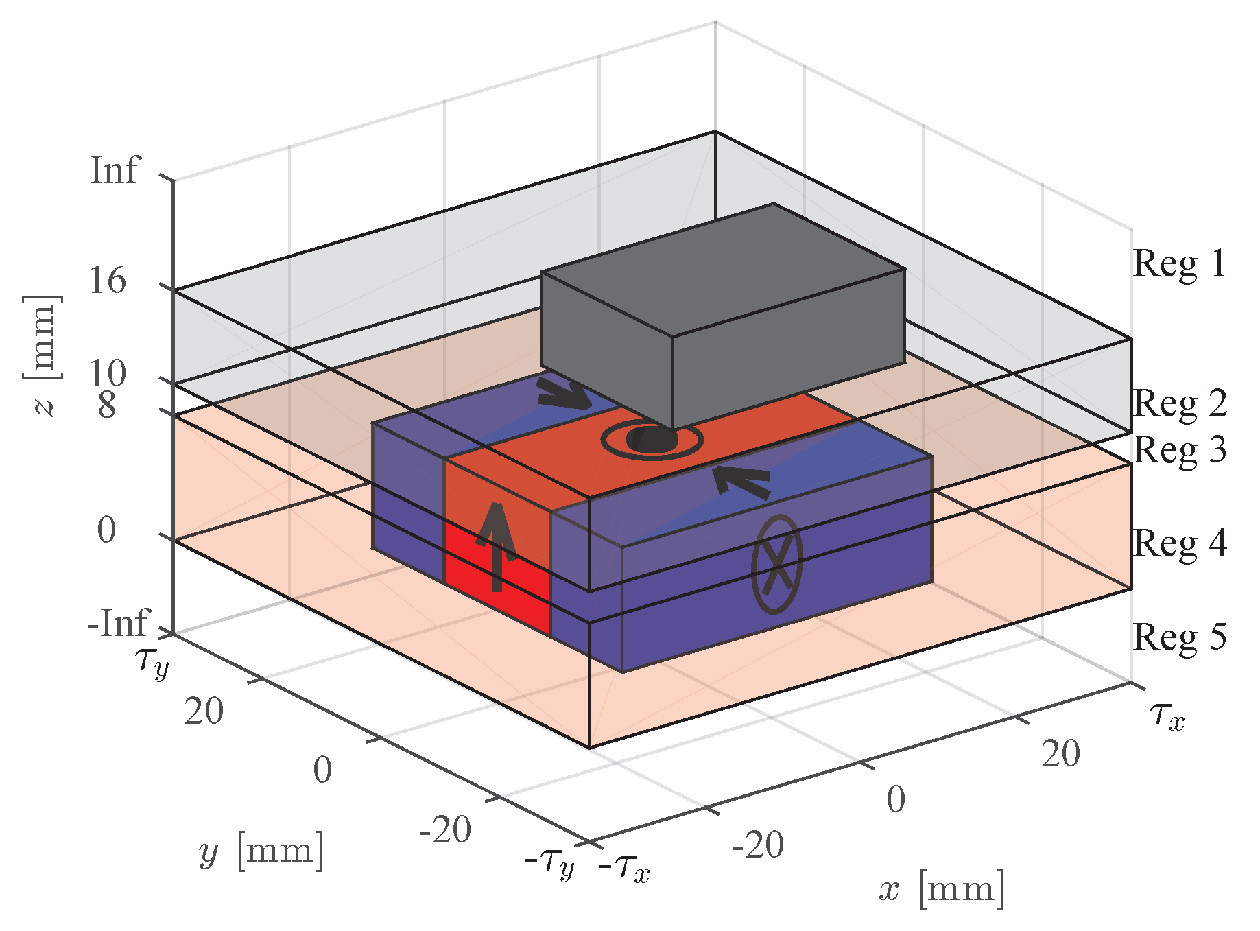
The scattering approach is applied to the electromagnetic configuration shown in Figure 2, where a rectangular slab of magnetic material is placed above three permanent magnets. The configuration is divided into five regions in the z-direction, as depicted in Figure 2. The model is periodic in both the x- and y- direction and the permeability inside Regions 2 and 4 varies as a function of position. The configuration was analyzed in [10], where also the expressions for the magnetic field components have been obtained and all geometric properties have been given. The magnetic properties are given in

Table 1. Model parameters.

Parameter	Value	Unit	Description
$B_{rem}$	1.3	T	Remanent flux density of the magnets
${\mu }_{r_{mag}}$	1.2	-	Relative permeability of the magnets
${\mu }_{r_p}$	800	-	Relative permeability of the plate in Region 2

. In [10], however, the unknowns where obtained by solving a linear system of equations as presented in (3).

Because only the magneto-static fields have to be considered for the configuration, the magnetic scalar potential, $\psi$, is introduced to obtain the expressions for the magnetic field quantities. In the boundary conditions, the continuity of this scalar potential and the z-component of the magnetic flux density are forced. Therefore, $\mathbf{u}={\mathbf{b}}_{\mathbf{z}}$ and $\mathbf{v}=\psi$ in (1) and (2), respectively. The expressions for ${\mathbf{b}}_{\mathbf{z}}$ and $\psi$ are described in [10]. Note that, for a problem where also an electric field exists, $\mathbf{u}$ and $\mathbf{v}$ would consist of the tangential components of the $\overrightarrow{H}$- and $\overrightarrow{E}$-field, respectively, and their size would be twice that compared to the current magneto-static problem. Hence, the expressions for $\mathbf{u}$ and $\mathbf{v}$ and their size depend on the problem at hand.

The number of harmonics that is used to calculate the solution to the configuration of Figure 2 is denoted by L. The number of harmonics used in the x- and y-directions is denoted by N and M, respectively, and thus the total number of harmonics $L=NM$. With the solving method of (3), the matrix that has to be inverted has a size of $8L\times 8L$, while with the scattering approach the maximum size of any matrix that is inverted is equal to $L\times L$. This means that the matrix size is reduced by 87.5%. Moreover, with the classical solving method, adding a region to the problem would mean that the matrix $\mathbf{E}$ becomes larger by $2L$ in both directions. In the scattering approach, the maximum size of any matrix would be $L\times L$, independent of the number of regions that makes the method especially beneficiary when the number of regions in a model is relatively large. The solving method using (3) is performed in Matlab R2017a using the command ‘A\b’, which means that the method of inversion is automatically chosen. It should be noted that properties reducing the computational effort of the inversion of a matrix, such as zeros in the off-diagonal entries and matrix symmetry are limited in the boundary condition matrix of (3), in contrast to the matrices inverted in (5), (6), (8), (9), (12) and (13).

In Figure 3a, the magnetic field strength, computed with the scattering matrix approach with a total of 6561 harmonics, in the center of Region 2 is depicted. The difference with the result computed by the finite element method (FEM) is shown in Figure 3b. In the FEM analysis, a total of 2,384,628 second-order mesh elements is used. It has been verified that, with the applied mesh, the error of the FEM (compared to a FEM result obtained with a denser mesh) has converged to an error less than 1%. In [10], a total of 1089 harmonics was used to obtain the same result. The maximum relative error with respect to FEM with 6561 harmonics is equal to 9.2%, where, computed with 1089 harmonics, the error was equal to 17.4%. For problems where the electromagnetic properties of a region are varying with a high spatial frequencies, the addition of harmonics can be necessary to obtain accurate field results.

Using the hardware available (quadcore Intel Core i7-4790 with 32 GB RAM), the computation time for the ‘classical’ solving method for a total of 1089 harmonics is equal to 20.4 s. With the developed scattering matrix approach, the computation time, for the same number of harmonics, is equal to 12.6 s. Hence, the number of calculations is increased in the scattering matrix approach, however, because all manipulations are performed on matrices of size $L\times L$, the computation time is not significantly increased or even decreased compared to the classical solving method. On the same hardware, the FEM analysis takes around 125 s to mesh and solve the electromagnetic problem. The semi-analytical approach obtains the results for the electromagnetic configuration of Figure 2 faster than the FEM; however, the solving time of the semi-analytical approach depends on the number of harmonics and number of regions in the model. This means that, for models where the geometry contains high spatial frequencies (relatively small details with respect to the periodic width), and the number of harmonics needs to be large to accurately compute the fields, and the advantage over FEM regarding computation time will decrease.

5. Conclusions

The paper presents the scattering matrix approach to solve the boundary conditions of a multiple region electromagnetic problem, with Fourier based solutions. Compared to the classical solving method, where all boundary conditions are collected in a single matrix, the scattering approach is more memory efficient. The boundary conditions for each region are reformulated, so that all unknowns, except the ones from the top and bottom region, can be removed from the problem. As a result, the maximum size of any matrix that is used during calculations is determined by the number of harmonics and, more importantly, independent of the number of regions inside the problem. Therefore, the scattering approach is especially beneficial for problems with a relatively large number of regions. Sources located inside a certain region of the electromagnetic configuration are taken into account in the described scattering formulation. Furthermore, due to the general formulation used, the approach can be used for a variety of electromagnetic problems with continuity boundary conditions between regions.

References

- Kawase, Y.; Yamaguchi, T.; Onogi, Y. Eddy current analysis of three-phase transformer using 3-D parallel finite element method. In Proceedings of the 2016 XXII International Conference on Electrical Machines (ICEM), Lausanne, Switzerland, 4–7 September 2016; pp. 2828–2832. [Google Scholar] [CrossRef]
- Mirzaei, M.; Binder, A.; Funieru, B.; Susic, M. Analytical Calculations of Induced Eddy Currents Losses in the Magnets of Surface Mounted PM Machines With Consideration of Circumferential and Axial Segmentation Effects. IEEE Trans. Magn. 2012, 48, 4831–4841. [Google Scholar] [CrossRef]
- Nasiri-Zarandi, R.; Mirsalim, M. Analysis and Torque Calculation of an Axial Flux Hysteresis Motor Based on Hyperbolic Model of Hysteresis Loop in Cartesian Coordinates. IEEE Trans. Magn. 2015, 51, 1–10. [Google Scholar] [CrossRef]
- Lubin, T.; Mezani, S.; Rezzoug, A. 2-D Exact Analytical Model for Surface-Mounted Permanent-Magnet Motors With Semi-Closed Slots. IEEE Trans. Magn. 2011, 47, 479–492. [Google Scholar] [CrossRef] [Green Version]
- Smeets, J.P.C.; Overboom, T.T.; Jansen, J.W.; Lomonova, E.A. Three-Dimensional Analytical Modeling Technique of Electromagnetic Fields of Air-Cored Coils Surrounded by Different Ferromagnetic Boundaries. IEEE Trans. Magn. 2013, 49, 5698–5708. [Google Scholar] [CrossRef]
- Dwivedi, A.; Singh, S.K.; Srivastava, R.K. Analysis of Permanent Magnet Brushless AC Motor Using Fourier Transform Approach. IET Electr. Power Appl. 2016, 10, 539–547. [Google Scholar] [CrossRef]
- Hannon, B.; Sergeant, P.; Dupré, L. 2-D Analytical Subdomain Model of a Slotted PMSM With Shielding Cylinder. IEEE Trans. Magn. 2014, 50, 1–10. [Google Scholar] [CrossRef]
- Custers, C.H.H.M.; Jansen, J.W.; Lomonova, E.A. 2-D Semi-Analytical Modeling of Eddy Currents in Multiple Non-Connected Conducting Elements. IEEE Trans. Magn. 2017, 53, 1–6. [Google Scholar] [CrossRef]
- Djelloul-Khedda, Z.; Boughrara, K.; Dubas, F.; Ibtiouen, R. Nonlinear Analytical Prediction of Magnetic Field and Electromagnetic Performances in Switched Reluctance Machines. IEEE Trans. Magn. 2017, 53, 1–11. [Google Scholar] [CrossRef]
- Custers, C.H.H.M.; Jansen, J.W.; van Beurden, M.C.; Lomonova, E.A. 3D Harmonic Modeling of Magnetostatic Fields Including Rectangular Structures with Finite Permeability. In Proceedings of the 2016 XXII International Conference on Electrical Machines (ICEM), Lausanne, Switzerland, 4–7 September 2016; pp. 1230–1236. [Google Scholar] [CrossRef]
- Djelloul-Khedda, Z.; Boughrara, K.; Dubas, F.; Kechroud, A.; Souleyman, B. Semi-Analytical Magnetic Field Predicting in Many Structures of Permanent-Magnet Synchronous Machines Considering the Iron Permeability. IEEE Trans. Magn. 2018, 54. [Google Scholar] [CrossRef]
- Cotter, N.P.K.; Preist, T.W.; Sambles, J.R. Scattering-Matrix Approach to Multilayer Diffraction. J. Opt. Soc. Am. A 1995, 12, 1097–1103. [Google Scholar] [CrossRef]
- Li, L. Formulation and Comparison of Two Recursive Matrix Algorithms for Modeling Layered Diffraction Gratings. J. Opt. Soc. Am. A 1996, 13, 1024–1035. [Google Scholar] [CrossRef]
- Rumpf, R. Improved Formulation of Scattering Matrices for Semi-Analytical Methods that is Consistent with Convention. Prog. Electromagn. Res. B 2011, 35, 241–261. [Google Scholar] [CrossRef]
- Onishi, M.; Crabtree, K.; Chipman, R.A. Formulation of Rigorous Coupled-Wave Theory for Gratings in Bianisotropic Media. J. Opt. Soc. Am. A 2011, 28, 1747–1758. [Google Scholar] [CrossRef] [PubMed]
- Pisarenco, M.; Maubach, J.; Setija, I.; Mattheij, R. Efficient Solution of Maxwell’s Equations for Geometries with Repeating Patterns by an Exchange of Discretization Directions in the Aperiodic Fourier Modal Method; CASA-Report; Technische Universiteit: Eindhoven, The Netherlands, 2012. [Google Scholar]
Figure 1.
Visual representation of the scattering formulation for a single region.
Figure 2.
Electromagnetic configuration consisting of three magnets with a slab of magnetic material above [10].
Figure 3.
Magnetic field strength in the z-direction on an -plane in the center of the region with magnetic material (Region 2). (a) calculated with the scattering matrix approach; (b) difference in calculated between the scattering matrix approach and the finite element method.