Rapid Modeling and Parameter Estimation of Partial Differential Algebraic Equations by a Functional Spreadsheet Paradigm


ExcelWorks LLC, Sharon, MA 02067, USA
Math. Comput. Appl. 2018, 23(3), 39; https://doi.org/10.3390/mca23030039
Submission received: 10 July 2018
/
Revised: 1 August 2018
/
Accepted: 1 August 2018
/
Published: 3 August 2018
(This article belongs to the Special Issue Computational Methods in Interdisciplinary Applications of Nonlinear Dynamics)
Abstract
:We present a systematic spreadsheet method for modeling and optimizing general partial differential algebraic equations (PDAE). The method exploits a pure spreadsheet PDAE solver function design that encapsulates the Method of Lines and permits seamless integration with an Excel spreadsheet nonlinear programming solver. Two alternative least-square dynamical minimization schemes are devised and demonstrated on a complex parameterized PDAE system with discontinues properties and coupled time derivatives. Applying the method involves no more than defining a few formulas that closely parallel the original mathematical equations, without any programming skills. It offers a simpler alternative to more complex environments which require nontrivial programming skill and effort.
1. Introduction
Excel, which is virtually available on every computer, is widely utilized for engineering and scientific applications thanks in part to its simplicity, hundreds of built-in mathematical functions, extensibility, and integrated graphing tools. In Reference [1], we demonstrated how Excel utility could be significantly enhanced to support computational calculus by expanding its built-in math functions with a new breed of calculus functions that also accept formulas as a new type of argument. The calculus functions are used in formulas, just like built-in math functions. For example, a calculus integration function accepts a formula and limits as inputs, and computes its integral value—much like an intrinsic math function accepts a number and computes its square root. Likewise, with appropriate input arguments, a differential system solver function computes and displays a formatted solution in an allocated array much like an intrinsic math function computes and displays an inverse of a matrix. The natural extension of built-in spreadsheet functions allows complete encapsulation of numerical algorithms for solving virtually any computational problem modeled by equivalent formulas using simple input/output pure function evaluation. Furthermore, the calculus functions can be naturally combined with Excel’s built-in Nonlinear Programming (NLP) solver for solving dynamical optimization problems.
In this paper, we exploit the merits of the calculus functions extension to develop a systematic and practical method for modeling and optimizing parameterized partial differential algebraic equations (PDAE). Specifically, we demonstrate how to carry out a least square dynamical minimization of the form
where is a parameter vector and is an observed value for a computed differential variable of the PDAE. We consider a general PDAE of one spatial dimension presented formally in the next section. We impose no restriction on the unknown parameters of the PDAE that are to be estimated. The parameters may include elements of a mass matrix coupling the temporal derivatives, initial conditions, or coefficients of the equations and boundary conditions, or even location points of boundary conditions. We further permit the PDAE to possess discontinuous properties that require imposition of special flux continuity boundary conditions across interfaces of discontinuity. A feature that is also incorporated in the PDAE example is presented later in the paper.
Algorithms for the solution of PDAE and function minimization are well developed and readily available in established computational packages [2]. A review of available software applications suitable for solving Equation (1) is beyond the scope of this paper, but, in general, utilizing a package, for instance MATLAB, to set up a dynamical optimization program with an underlining differential equation system involves coding skill and effort [3]. This paper demonstrates a straightforward method combining the Excel NLP solver, which is based on the Generalized Reduced Gradient algorithm [4], with a calculus function encapsulating the Method of Lines (MOL) [5] to carry out the dynamical minimization Equation (1) with only basic Excel spreadsheet skills. Our devised method requires no more than defining a few analogues formulas that closely parallel the PDAE.
Finite difference methods have been widely applied for solving partial differential equations (PDE) in the spreadsheet [6,7,8]. In particular, numerous applications of Excel have been reported for solving environmental problems and groundwater management models, including utilizing Excel NLP solver for aquifer parameter estimation using inverse modeling techniques [9,10,11,12,13,14]. The underlining PDE in such models are often based on the incompressible flow equations in a confined aquifer that is amenable for a finite difference approximation on a spreadsheet-structured grid [13]. Review of these applications is beyond the scope of this paper, but in general, these methods are founded on utilizing the spreadsheet explicitly as the computational grid for the finite difference scheme; in essence, confounding inputs, numerical algorithmic procedure and results. These methods are tightly coupled to the underlining discretized PDE model; they are designed to solve and cannot be utilized as general-purpose PDE solvers.
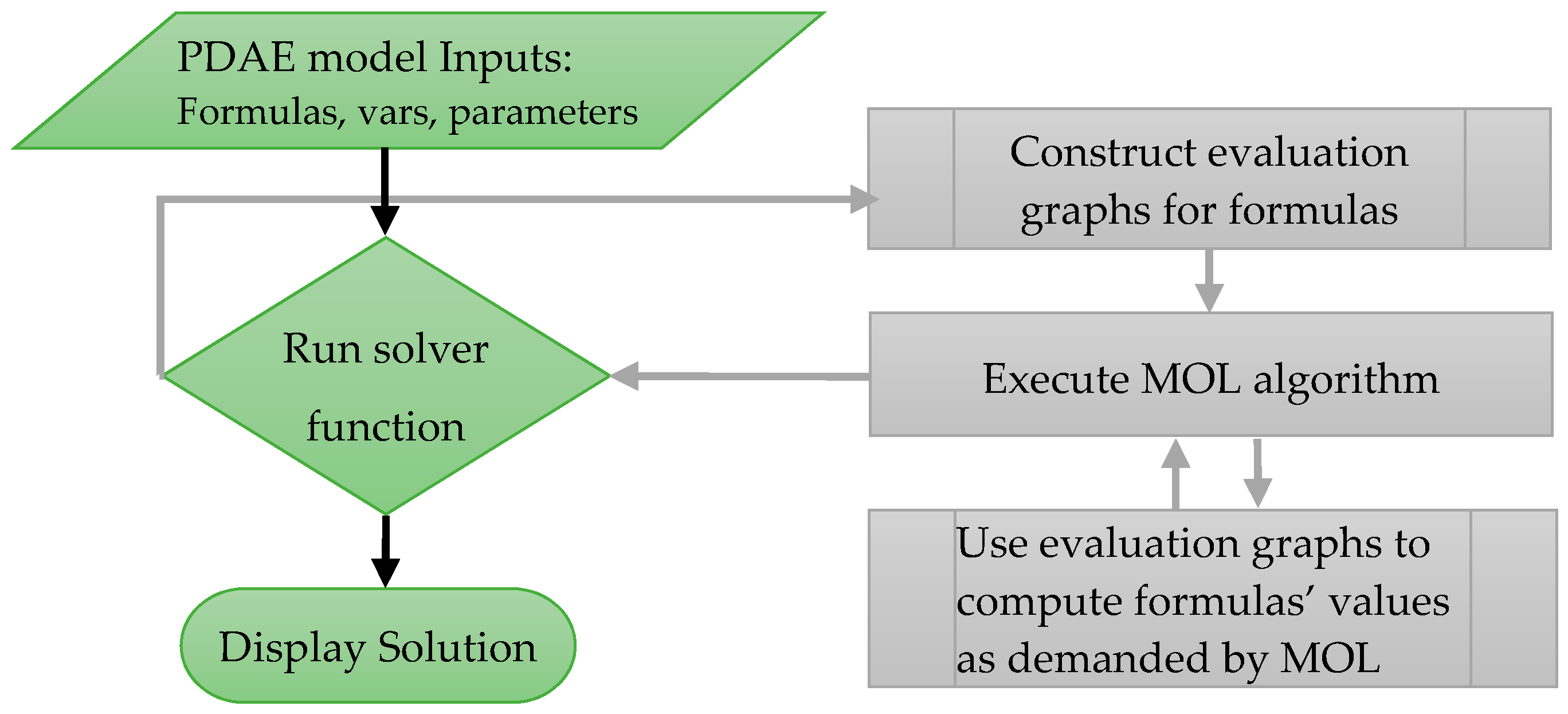
To the best of our knowledge, no prior work has demonstrated a practical spreadsheet method for dynamical optimization of a general nonlinear PDAE with discontinued properties. To enable the devised method of this paper, we rely on an unconventional approach for exploiting the spreadsheet computational engine [15,16,17], which permits us to encapsulate the MOL in a mathematically pure spreadsheet function suitable for natural integration with the Excel NLP solver. The PDAE solver function, named PDASOLVE, behaves just like any built-in math function, and operates according to the flowchart logic of Figure 1, with a clear divide between model input, MOL procedure, and output solution. Unlike traditional methods, PDASOLVE does not modify its input, which permits employing it in a functional dynamical optimization paradigm. In this paradigm, the authority to modify the parameters of the PDAE system is confined to the outer NLP solver, whereas the inner PDASOLVE function is simply evaluated repeatedly as directed by the NLP algorithm. Moreover, decoupling the MOL procedure from the spreadsheet grid facilitates supporting more general PDAE models with discontinuous properties as demonstrated in Section 4.
The remainder of this paper is organized as follows: In the next section, we present a formal statement of the PDAE system, as well as a description of the MOL solution strategy. In Section 3, we describe PDASOLVE function design, its input and output formats. In Section 4 we present two examples including detailed demonstration for building a spreadsheet model, solving and verifying the solution for a parameterized multiregion PDAE system with discontinued properties. In Section 5, we demonstrate how to optimize the PDAE model parameters for best fit with observed values utilizing the Excel NLP solver command. This section also includes numerical experiments aimed at investigating relative effects of parameters, including how to parameterize initial conditions. In Section 6, we demonstrate how to carry out the unconstrained minimization by an alternative spreadsheet pure solver function based on the Levenberg–Marquardt (LM) algorithm [18,19]. An Appendix A is included with a summary of practical considerations for using the devised spreadsheet method. The paper assumes the reader has only elementary familiarity with spreadsheet concepts.
2. Description of PDAE System and Solution Method
We consider a transient PDAE of one spatial dimension , in the interval , subject to initial, and various combination of boundary conditions as stated in Equations (2)–(7).
are the state differential variables with corresponding first and second derivatives and . is a mass matrix that may be singular, in which case the system is differential-algebraic. Each right-hand-side function is generally a nonlinear function, which may be defined over only a subregion of the system’s domain . An initial condition, , is required for each dependent variable .
2.1. Boundary Conditions
Boundary conditions are required only for differential variables. Generally, for a well-posed system, if the equations depend only on the first derivative of a differential variable, then only one boundary condition implicating the variable is needed. On the other hand, if the equations depend on the second derivative of a differential variable, then two boundary conditions or one mixed boundary condition (e.g., convective heat transfer) implicating both the variable and its derivative are needed. Permitted boundary conditions are classified into four types:
- Dirichlet: a constant or time-dependent boundary condition, , specified for an individual state variable .
- Neumann: a constant or time-dependent boundary condition, , specified for an individual state variable derivative .
- Robin: a general boundary condition involving an algebraic expression of state variables and possibly their first derivatives.
- Continuity: a special condition that enforces continuity of a flux across an interface separating two regions with discontinuous material properties. A flux is defined as the product of a property , and the first derivative of a differential variable.
2.2. Solution Strategy
We use the MOL [5] to solve the above system, which transforms the PDAE system into an ordinary differential algebraic equation (DAE) system that can be solved by well-developed integration schemes. The main steps required to implement the MOL are described below:
- An initial spatial grid consisting of fixed geometrical points for the problem is constructed. The geometrical points include system equation subregions’ end points, , and boundary condition points. The grid is then refined to satisfy that a minimum number of nodes is generated between any two consecutive geometrical points, as well as the distance between any two nodes is within a specified limit.
- Mapping data structures are constructed to record topological relationships between grid nodes, differential equations, regions and boundary conditions. The data structures support efficient retrieval of information pertaining to a grid node, including whether it is boundary condition node, an interior node, or a region end point, as well as its immediate neighbors and associated differential equations.
- A higher order finite difference scheme is used to approximate the first and second derivatives in terms of the state variables on the spatial grid. Since grid spacing across geometrical points may vary, a variable-step difference scheme is used when neighboring nodes have nonuniform spacing. Dirichlet and Neumann boundary conditions are incorporated at this step by substituting their direct values into the difference scheme.
- The spatial discretization in the previous step eliminates one degree of freedom, which transforms the PDAE into a banded initial value DAE system that can be integrated on an independent time grid using an appropriate DAE algorithm. In particular, we employ the RADAU5 algorithm, which is based on an adaptive implicit Runge–Kutta scheme of order five and supports implicit time-coupled DAE equations [20].
- Robin and Continuity-type boundary conditions are discretized in similar way but imposed as additional algebraic equations on the DAE system. In particular, for flux continuity conditions, each side of Equation (7) is computed using a one-sided difference scheme, and the residual is imposed as an algebraic constraint of zero value at the respective nodes.
3. Description of PDASOLVE Function Interface
3.1. Input Parameters
PDASOLVE function design represents an evolution of an original PDASOLVE function design introduced in Reference [21] using a collocation method that was limited to explicit PDE with continuous properties. The new algorithmic enhancements include the ability to specify continuity boundary conditions at arbitrary locations, the ability to specify subregions for the system equations, the ability to include algebraic constraint equations, and the ability to supply a mass matrix. PDASOLVE interface takes the following form with nine input parameters, the first five of which are required and the last four are optional with default settings [22]:
=PDASOLVE(eqns, vars, bcs, xdom, tdom, [M, regions, tols, options])
The input parameters are described below:
Required parameters
- Reference to formulas corresponding to the system right-hand-side functions including algabraic constraint equations if present.
- Reference to the system variables in the following order .
- Reference to a three-column array containing definitions for the system’s boundary conditions. The first column specifies the positions of the boundary conditions; the second column specifies the types that are identified by any of the letters ‘D’, ‘N’, ‘R’ or ‘C’, corresponding respectively to Dirichlet, Neumann, Robin, or Continuity; and the third column specifies the boundary condition formulas defined with respect to zero on one side.
- Spatial domain limits and output control.
- Time interval limit and output control.Optional parameters which may be omitted if not applicable.
- Mass matrix or number of algebraic equations in PDAE with identity mass matrix.
- Reference to a two-column array containing end points for each equation’s subregion.
- Tolerances for the time integration scheme.
- Reference to a two-column array containing key/value pairs for algorithm settings, grid control, and output solution format.
Proper definition and use of the input parameters is illustrated in the examples presented in Section 4.
3.2. Output
Formula (8) is evaluated in the spreadsheet as a standard array formula in an allocated array of sufficient size to hold the solution result. The layout of the solution can be either a transient or snapshot format. In the snapshot format, shown in Figure 2, the spatial output points are listed in the first column of the array, whereas the temporal output points are listed in the first row of the array, and the solution state variables, (including derivatives if requested) are listed in repeated blocks of columns. This format is convenient for plotting a spatial-distribution (snapshot) view of the solution at different time points. In the transient layout, the order of x and t is swapped to allow for direct plotting of the variables’ transient trajectories at selected spatial points. Switching between the two formats is controlled via optional parameters [22]. By default, the solution is reported at uniform intervals for time and space, determined by the allocated size of the output array. However, via optional parameters, the output solution can be customized in multiple ways, for example, by specifying the exact time or space output points, by specifying the size of the division for time or space, and by requesting to report the first and second derivatives of the state variables. Some of these options are utilized in the examples of next section.
4. Numerical Examples
In the following subsections, we utilize the PDASOLVE function to solve two problems: a single-region continuous PDE system; and a discontinuous multiregion PDAE system. The examples were selected to illustrate the systematic procedure, as well as verify the accuracy of obtained solutions. The computations were carried on a standard laptop computer with an Intel i7 four-core processor at 2.70 GHz running Microsoft Windows 10 and Excel 2016 with ExceLab calculus add-in [22], which contains the implementation of PDASOLVE and enables the function in Excel. A supplementary Excel workbook containing the solved examples is available for downloading.
4.1. A Continuous PDE System
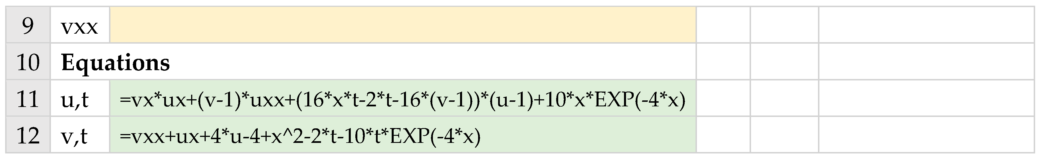
Our first example considers a nonlinear PDE system of Equations (9) and (10), which has a known exact analytical solution for the configuration shown in Table 1. The exact solution [23] is given by Equations (11) and (12). This example serves two purposes: to illustrate how to rapidly model and solve a PDE system in Excel, as well as to verify the accuracy of the numerical solution obtained with PDASOLVE.
4.1.1. Spreadsheet Model
It is convenient to define and work with named cell variables rather than work with raw cell addresses, such as A1. Referring to Figure 3, we started by naming cells B2:B9, respectively, as t, x, u, v, ux, vx, uxx, and vxx to serve as the system variables. Variables u and v are assigned the initial conditions values of one which, in general, can be formulas of the spatial variable x. Using the named variables, the equivalent formulas for the system right-hand-side Equations (9) and (10) were defined in cells B11:B12, and the left (x = 0) and right (x = 1) boundary conditions were defined in the matrix C3:E6. Note that each boundary condition is represented by an equivalent formula with respect to zero on one side, and assigned the appropriate type. In this example, we have Dirichlet at x = 0 and Robin at x = 1.
4.1.2. Solution by PDASOLVE Function
Next, we defined PDASOLVE Formula (13) in allocated array F1:L23. In the formula parameters, we passed the colored ranges of Figure 3, which include the system variables, equations, and boundary conditions matrix, as well as two constant arrays in parameters 4 and 5, which define the system’s spatial and temporal domains.
=PDASOLVE(B11:B12, B2:B9, C3:E6, {0,1}, {0,2})
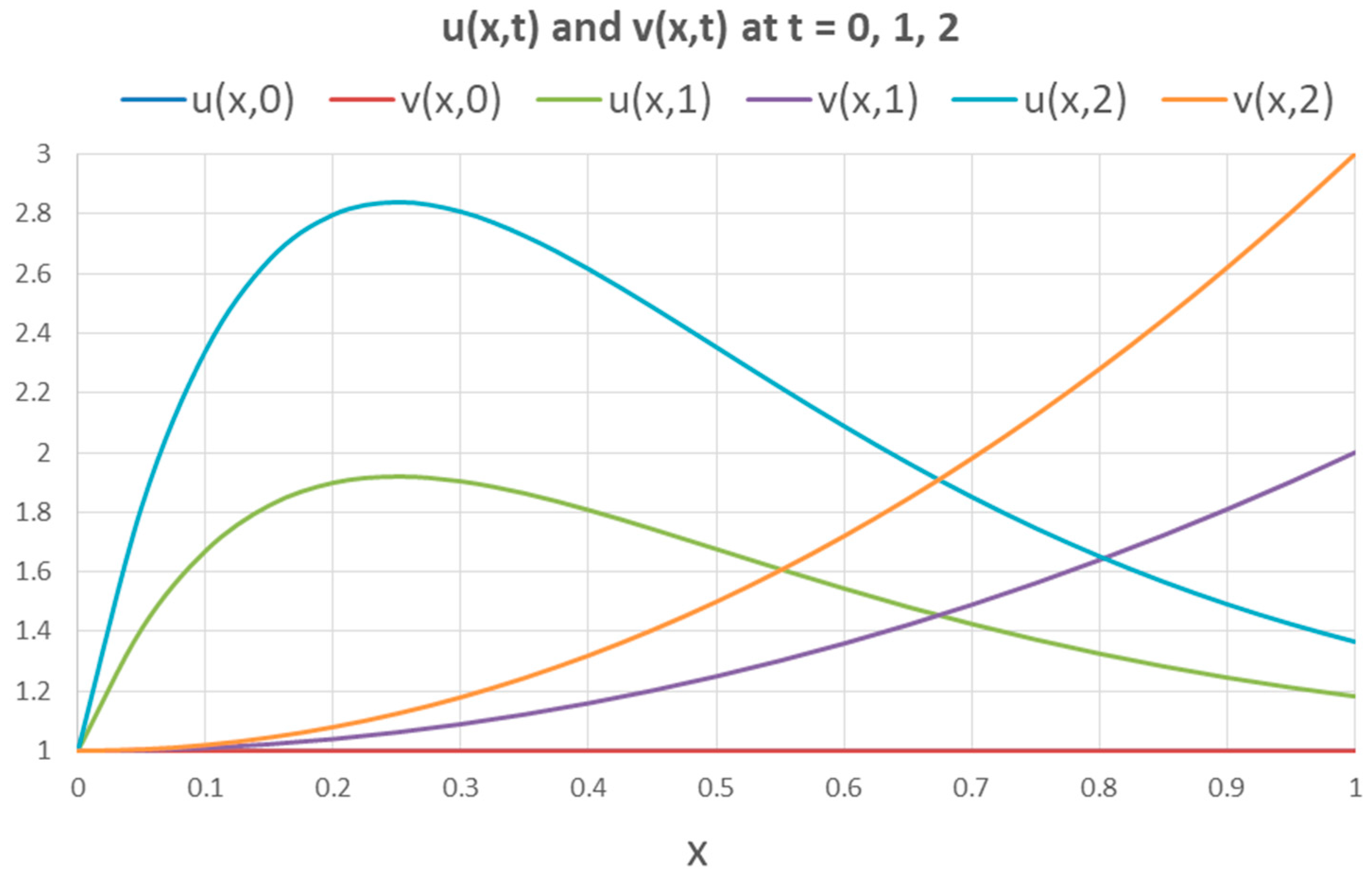
Evaluating Formula (13) as an array formula by pressing Ctrl+Shift+Enter simultaneously populated the allocated array F1:L23 by the formatted solution shown in Figure 4 under one second of computing time (the measured CPU clock time was 0.852 s). Snapshots of u and v profiles at different times are plotted in Figure 5.
The numerical solution computed by Formula (13) with the default discretization settings for PDASOLVE agrees well with the analytical values computed by Equations (11) and (12) as shown in Table 2, which lists the absolute errors. Improving the accuracy is possible with optional settings and is demonstrated in the next example.
4.2. A Discontinuous PDAE System
4.2.1. Mathematical Model
We considered a parameterized PDAE system of Equations (14)–(16), constructed to model a hypothetical battery with three regions as shown in Figure 6.
Equation (14) is defined in the cathode region only, Equation (15) is defined in all three regions, and Equation (16) is defined in the anode region only. The three equations are coupled by a mass matrix M. This example represents a model with some unknown design parameters to be estimated, and is intended to illustrate the solution procedure rather than the physics, as well as serve as a template upon which other models can be defined
Definitions for the discontinuous property functions and the source function are given by Equations (17)–(20). and depend, respectively, on parameters and , with initial values listed in Table 3, which also includes definitions for the initial conditions and values for the geometrical points and .
The mass matrix M is defined by Equation (21) and depends on the off-diagonal parameter with initial value given in Table 3.
4.2.2. Boundary Conditions
Table 4 lists the boundary conditions at the spatial domain’s end points and regions’ interior interfaces for System (14)–(16). Two continuity conditions are required for the flux at both and because of the discontinuity in values across the different regions. Note that and are not defined in region 2, so no continuity conditions are required for their fluxes.
4.2.3. Problem Objective
System (14)–(16) depends on a number of fixed and unknown design parameters, which are to be estimated. The design parameters are listed in Table 3, and include the off-diagonal mass matrix element , and the coefficients and , which have been assigned initial values. The objective is find the best estimates for the design parameters, so the given model accurately predicts observed values for measured at . The given observed transient values for are plotted in Figure 7.
4.2.4. Spreadsheet Model
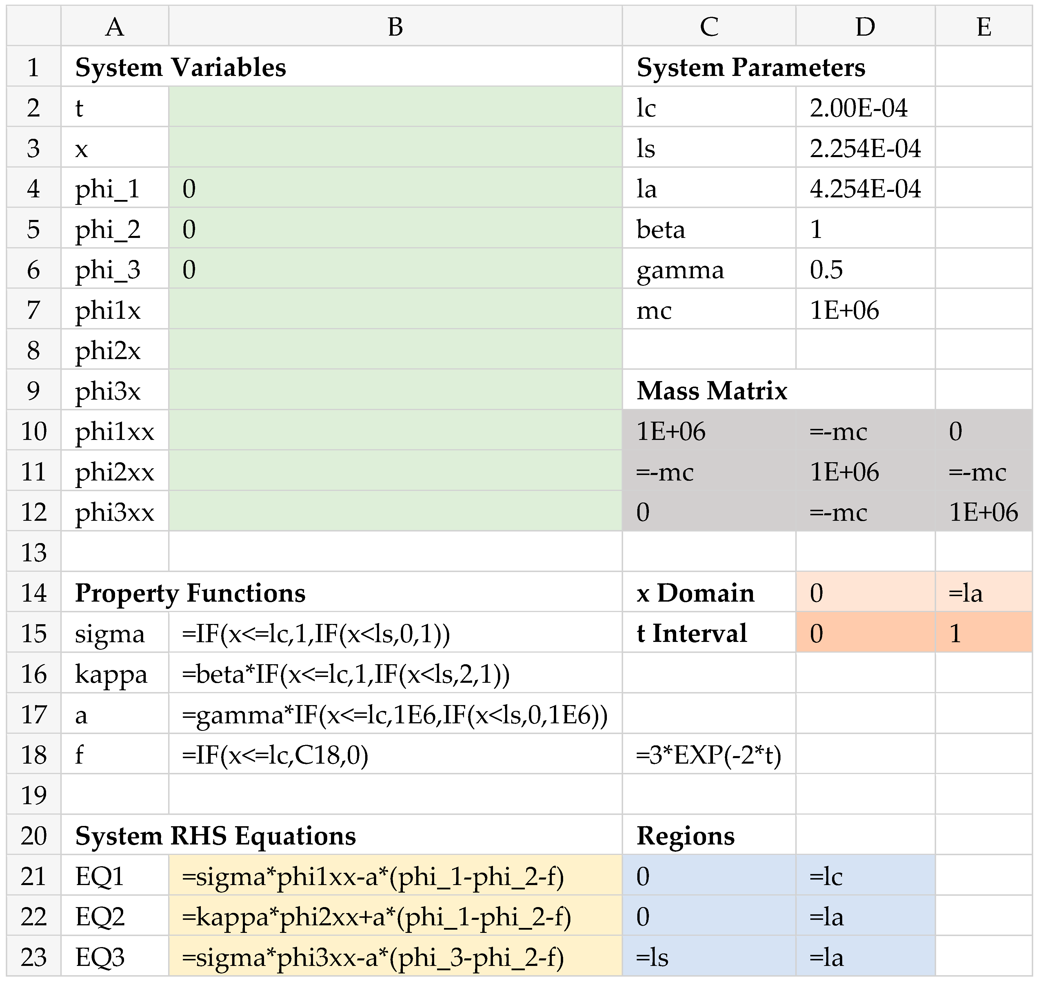
Modeling System (14)–(16) in the spreadsheet by equivalent formulas and variables is straightforward with a few ordered steps. Referring to Figure 8, we named cells B2:B12 as t, x, phi_1, phi_2, phi_3, phi1x, phi2x, phi3x, phi1xx, phi2xx, phi3xx to represent, respectively, the system’s variables . We then defined the initial conditions for phi_1, phi_2, and phi_3, which are simply zero, but in general, may be formulas of the variable x. Likewise, we named cells D2:D7 as lc, ls, la, beta, gamma, and mc to represent, respectively, and , and assigned their numerical values given in Table 3. We defined the mass matrix M as shown in range C10:E12 and chose to parameterize the off-diagonal term with mc rather than store its numerical value, since we intend to use it as a design variable in the ensuing optimization exercises. Using the standard IF statement, we defined the property and source functions , ,, and as shown in cells B15:B18, as well as assigned them the names sigma, kappa, a, and f, respectively. Using the named variables, we defined the system (14)–(16) right-hand-side equations by the equivalent formulas shown in cells B21:B23. Next to each equation, we defined the corresponding spatial region as shown in C21:D23. The spatial domain and time interval are defined in ranges D14:E14, and D15:E15, respectively.
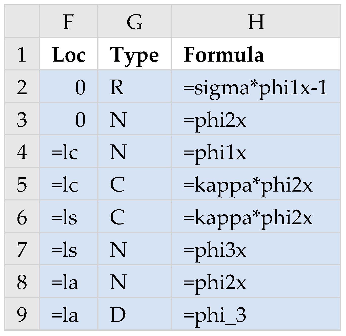
To complete the model definition, we defined the boundary conditions, listed in Table 4, using a three-column range F2:H9 as shown in Figure 9. The first column specifies the x locations of the boundary conditions, the second column specifies the types that are identified by any of the letters ‘D’, ‘N’, ‘R’ or ‘C’, which map to Dirichlet, Neumann, Robin, or Continuity. The third column specifies the boundary condition formulas that are arranged with respect to zero on one side.
4.2.5. Computing the Solution by PDASOLVE Function
To aid readability for the PDASOLVE formula, we defined, using Excel Name Manager, identifier names as listed in Table 5 for the colored spreadsheet ranges shown in Figure 8 and Figure 9, which represent input arguments to PDASOLVE spreadsheet function.
The input ranges are passed to PDASOLVE function in the order shown in Formula (22). We skipped over the eighth optional parameter (to use default tolerances) and specified in the ninth optional parameter a control key/value pair, (using constant array syntax for convenience), which instructs the solver to report the solution using the transient format. This format is convenient for generating transient plots.
=PDASOLVE(Eqns, Vars, BCs, xDom, tDom, M, Rgns, {“FORMAT”,”TCOL1”})
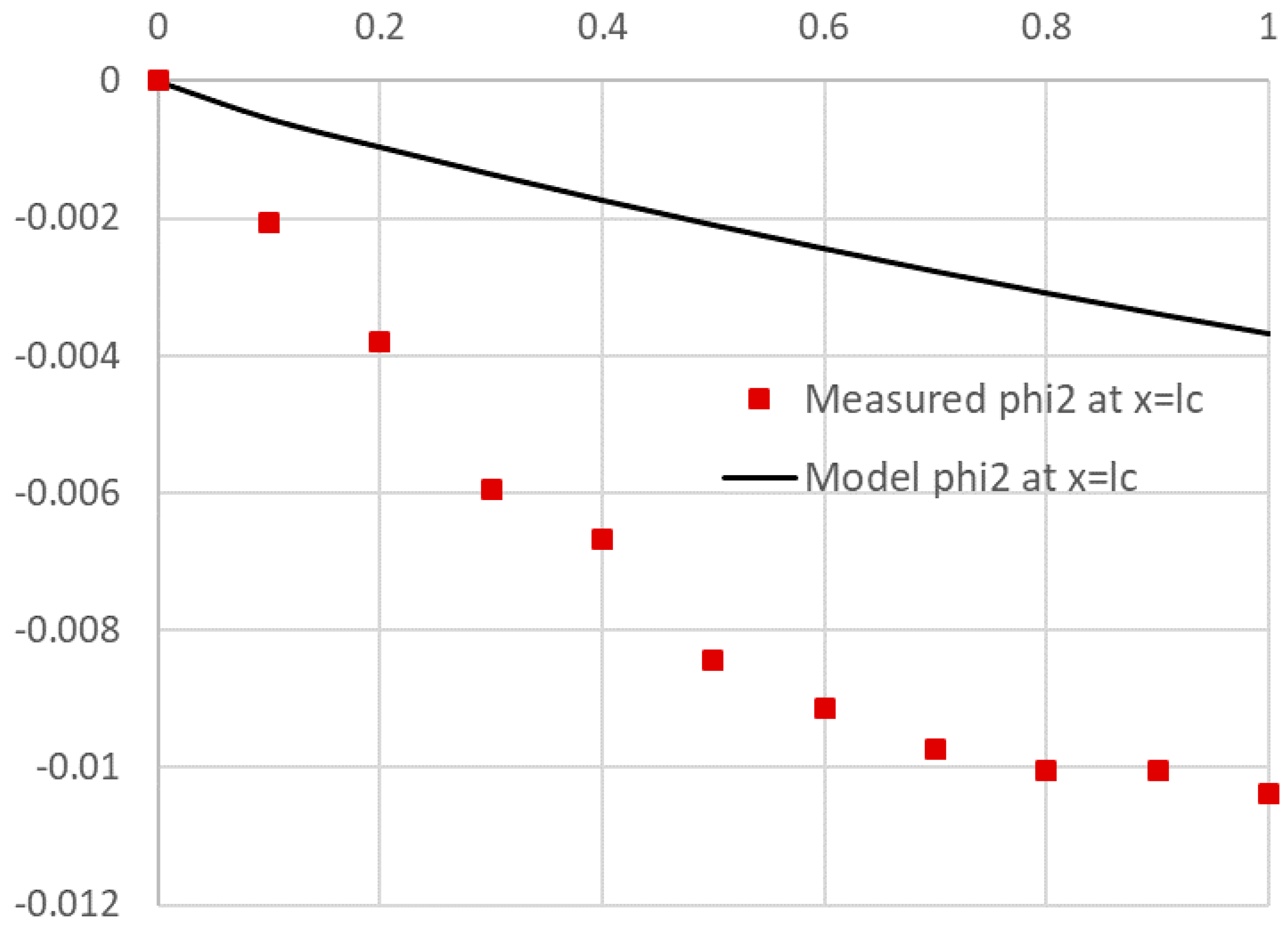
PDASOLVE Formula (22) is run as a standard array formula in a preallocated range of sufficient size to hold the solution result. By default, it reports values for the state variables at uniform intervals for time and space determined by the size of the allocated solution array. In the first run, we evaluated array Formula (22) in the selected range G15:S27 (by pressing Ctrl+Shift+Enter), and obtained, almost instantaneously (the measured CPU time was 0.477 s), the solution shown in Figure 10. The output range size was selected such as to report the solution only at the geometrical points of the spatial domain (regions ends) with 10 divisions of the time interval. The computed values for phi_2 at x = lc are highlighted in the figure and plotted in Figure 11, along with the observed values which exhibits unacceptable divergence. However, prior to optimizing the model, we demonstrate next how to verify the numerical solution accuracy and, in particular, verifying that the flux continuity conditions are satisfied.
4.2.6. Verification of Continuity Boundary Conditions
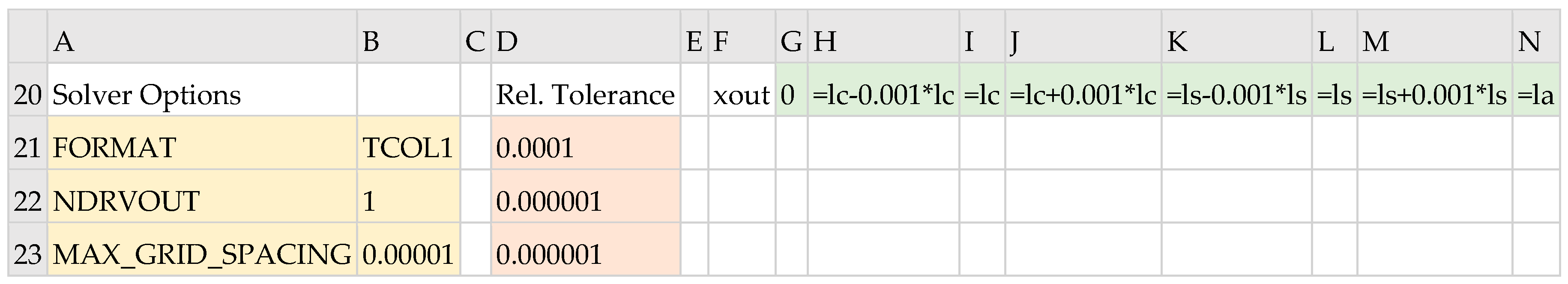
The default solution result as obtained in Figure 10 is insufficient to verify that the flux continuity conditions , and are satisfied at and . Therefore, we illustrate use of additional optional parameters to PDASOLVE in order to: first, report the first derivatives at custom spatial points just before and after and , and, second, enhance the solution accuracy. Figure 12 shows the definition of new optional parameters consisting of: the custom output points defined in G20:N20, which is named as xOut; the relative tolerance vector for the three state variables defined in D21:D23, which is named as rTols; and a set of key/value pairs defined in A21:B23, which is named Cntrls. The keys include NDRVOUT with a value of 1, which instructs the solver to report the first derivative variables in the output, and MAX_GRID_SPACING, which ensures that the maximum distance between computational spatial grid nodes does not exceed the specified value of 1.0 × 10⁻⁵. The initial PDASOLVE Formula (22) has been modified as shown in Formula (23), in which we pass the new optional parameters as defined in Figure 12.
=PDASOLVE(Eqns, Vars, BCs, xOut, tDom, M, Rgns, rTols, Cntrls)
Evaluating array Formula (23) requires a larger array size to hold the additional output derivatives. The minimum number of columns can be determined by evaluating Formula (23) in one cell initially, which reports an error message with the required minimum array size for output. In this case, it is 49 columns. Figure 13 displays a portion of the formatted output solution around , which shows the values of phi2x just before and after x = 0.000225 (ls). A quick inspection of the values shows that the ratio is satisfied. The computed ratios at and for all time points are shown in Table 6. With the increased grid size, the measured CPU time was 1.445 s for this run.
5. Parameter Estimation via Dynamical Minimization
We aim to compute optimal values for the design parameters , and which minimize the sum of square residuals between the model predictions and observed values for at . The solution to the least square parameter estimation problem can be stated as the optimum of an unconstrained dynamical minimization problem of the form:
where is an observed transient value of at , and is the computed value for specified values of the parameters , and . The dynamical minimization problem (24) can be solved by combining the Excel built-in NLP solver with PDASOLVE in a simple functional paradigm. Key to the proper execution of the functional formulation is the purity of PDASOLVE function, and the Automatic Calculation Mode of the spreadsheet. Any modification to the design parameters by the outer NLP solver triggers reevaluation of the inner PDASOLVE solution, and any dependent objective and constraint formulas, in the proper order. In practice, there are three structured tasks to solve the dynamical minimization problem (24), the first of which we have already accomplished in the previous sections, but emphasize below again:
- Task 1:
- We obtain an initial solution of the parameterized PDAE model in an allocated array of the spreadsheet as shown in Figure 10. Depending on the problem requirements, it may be advantageous to switch between a transient or snapshot format for the output layout, as well as customize the output to display values of interest.
- Task 2:
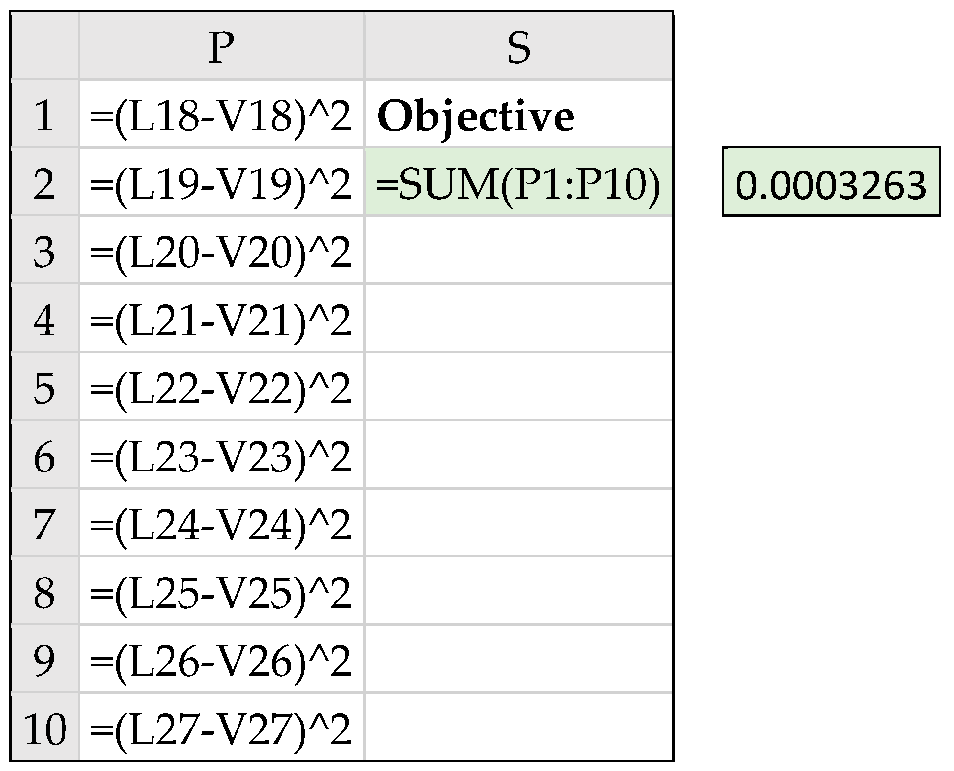
- Based on the output result obtained in Task 1 and given observed values, we define an objective formula to be minimized. The objective formula calculates the summation of the square residuals between the observed values and their corresponding computed values from the output result. The spreadsheet is perfectly suited for performing this task given its AutoFill feature and built in math function SUM. Definition of the objective formula for our example is shown in cell S2 of Figure 14. The definition is based on the computed values shown in Figure 10 and observed values stored in range V18:V27.
- Task 3:
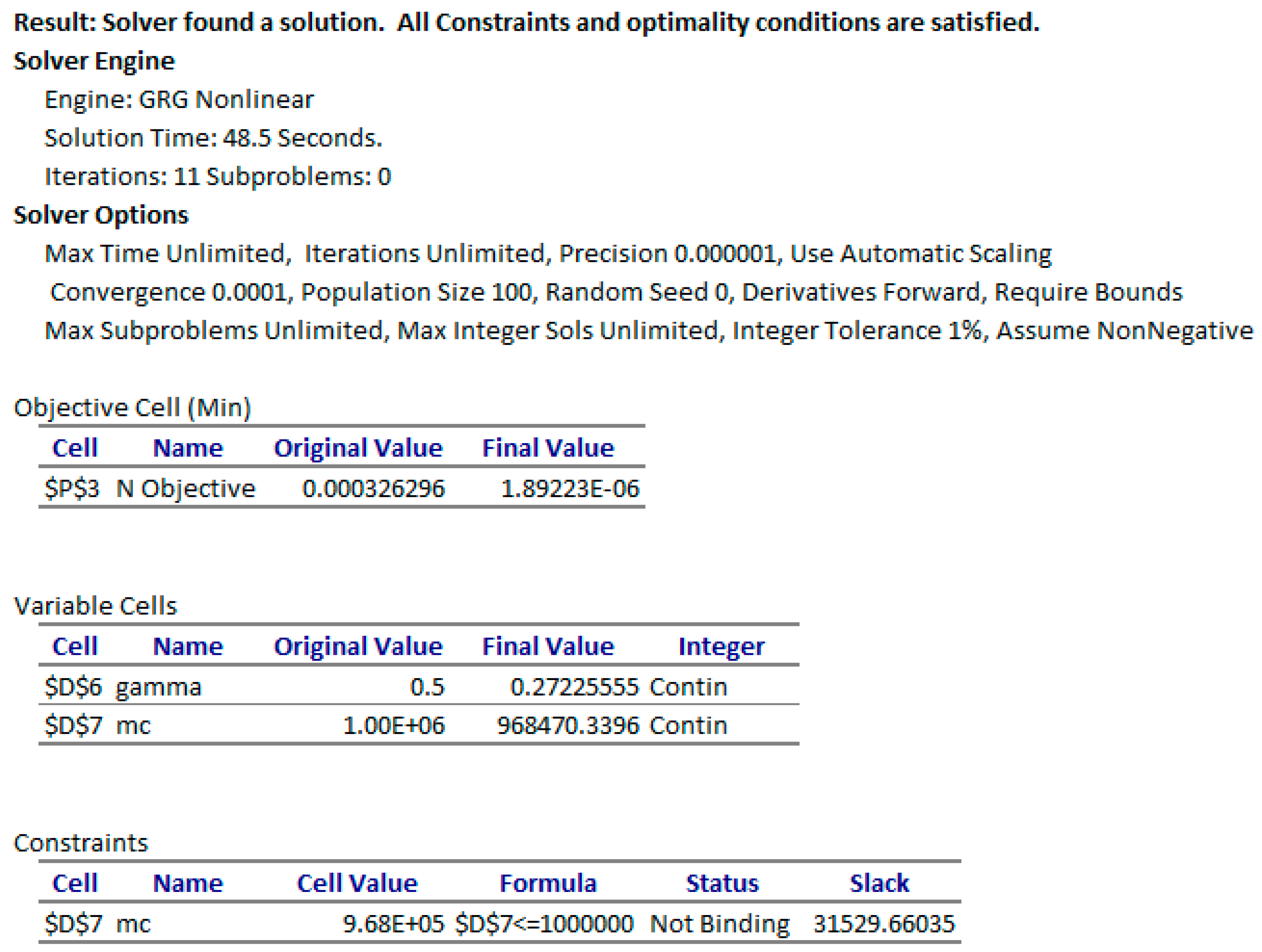
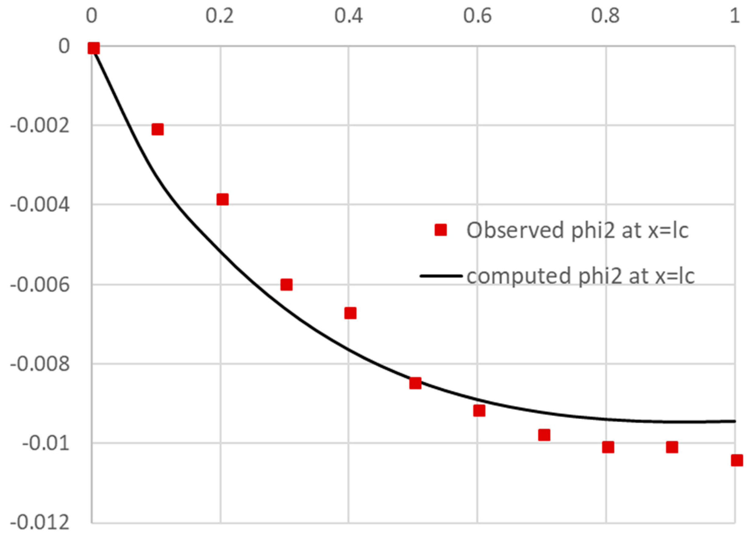
- The remaining task is to configure and run the Excel NLP solver command. Excel solver is invoked from the Data Tab in the Ribbon and displays a simple dialog, which can be configured to minimize or maximize an objective formula by changing variables cells, subject to added constraint formulas. Figure 15 shows the configuration for our example, where we select to minimize the objective Formula S2, by varying gamma and mc variable cells, subject to the upper bound constraint mc ≤ 10 × 106. The bound constraint was added for numerical stability since larger values for the off-diagonal mass matrix element leads to a divergent system. We have also imposed the condition that gamma and mc are nonnegative as shown in Figure 15. We ran the solver that reported a feasible solution in about 48 s of computing time as shown in the Answer Report generated by the solver in Figure 16. The Answer Report shows the original objective value of 3.26 × 10⁻⁴ has been reduced to 1.89 × 10⁻⁶ in 11 iterations. Upon accepting the solution, Excel automatically updates the spreadsheet to reflect the optimal computed values. The optimized PDAE solution for phi2 is shown in Figure 17, exhibiting excellent agreement with observed values.
5.1. Relative Influence of Design Parameters
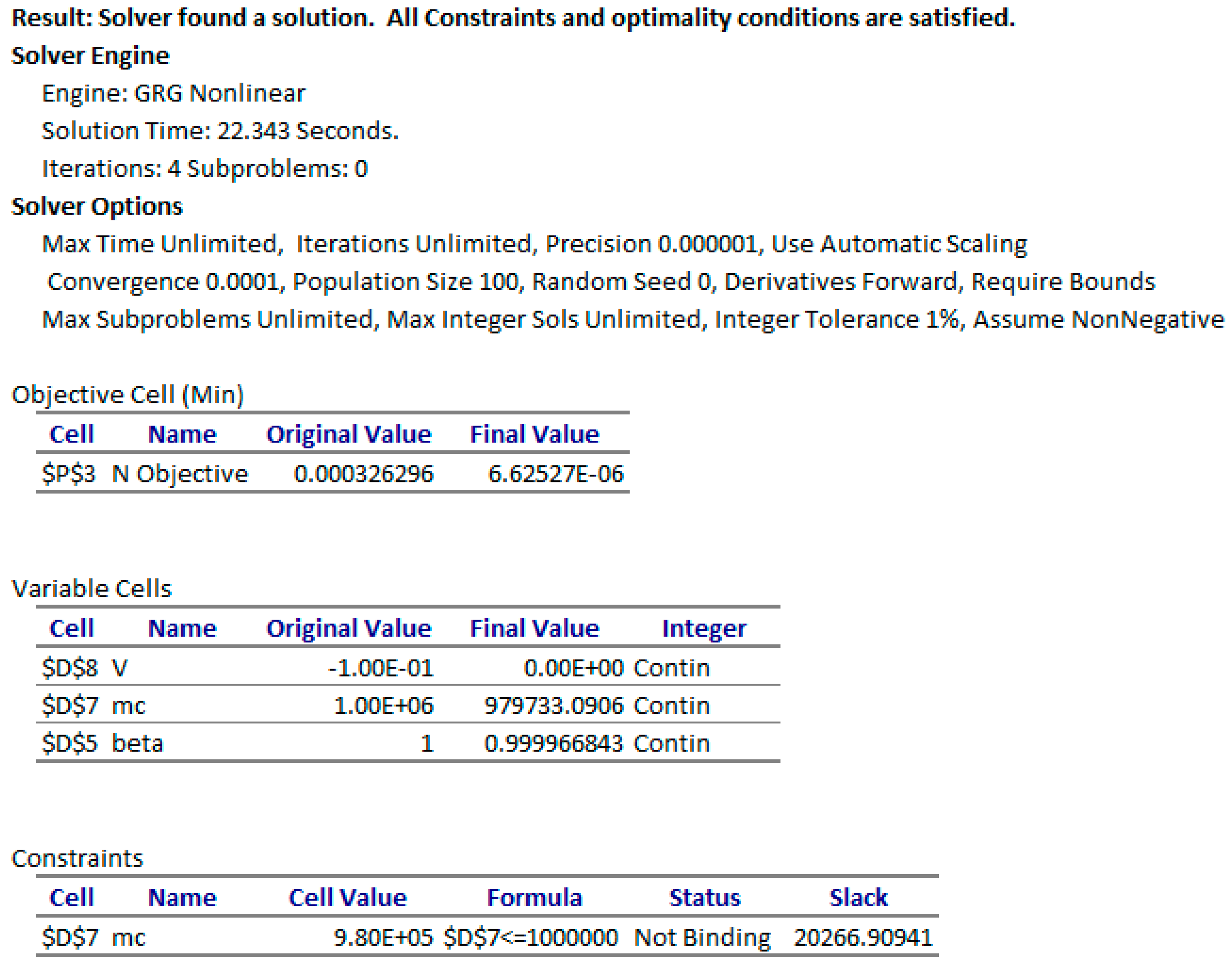
It is interesting to investigate the individual influence of , and on the quality of the least-square fit. In the first experiment we hold fixed at its default value of 0.5 but vary only . The NLP solver converges to the solution shown in Figure 18 and plotted in Figure 19. The new objective value of 6.625 × 10⁻⁶ is higher than obtained earlier at 1.89 × 10⁻⁶, which reflects the less optimal curve fit shown in Figure 19. Next, we fix at its initial value of 1.0 × 10⁶ but vary alone. The NLP solver solution was unacceptable with a value of zero for at insignificant reduction of the original objective value from 0.00033 to 0.00028. Therefore, we conclude that both and are critical for obtaining the best fit, even though carries the larger influence on the optimal result.
5.2. Investigating Effect of Initial Condition and Additional Parameters
Often, one end of a system, initially at a uniform initial condition, is suddenly subjected to a different condition. Here we demonstrate how to define and parameterize such an initial condition. Specifically, we assume that the initial condition for is defined as follows
where is design parameter with initial value of −0.1. In this experiment, we will treat and as the design parameters while holding . To incorporate Equation (25) into the spreadsheet model shown in Figure 8, we simply introduce a new variable named V in cell D8 with an initial value of –0.1, and replace the zero-initial condition value for phi_2 in cell B5 with the new formula
= IF(x = 0, V, 0)
We configured the NLP solver to vary the design variables V, mc, and beta. The Solver converges essentially to the same result obtained in the last experiment at nearly the same cost by finding V at 0 and near 1 as shown in the Answer Report of Figure 20.
6. Alternative Spreadsheet Dynamical Minimization Strategy
One of the best-known algorithms for unconstrained minimization problems and least square fitting is the LM [18,19]. Unfortunately, it is not available with the standard Excel NLP solver, which is based on the Generalized Reduced Gradient algorithm [4]. Utilizing the same design mechanism of Figure 1, we implemented the LM algorithm in a pure spreadsheet solver function, NLSOLVE. Purity of NLSOLVE permits it to be combined with PDASOLVE to implement an efficient dynamical functional paradigm as an alternative to using Excel NLP solver. NLSOLVE has the following simple interface:
=NLSOLVE(constraints, variables, [options])
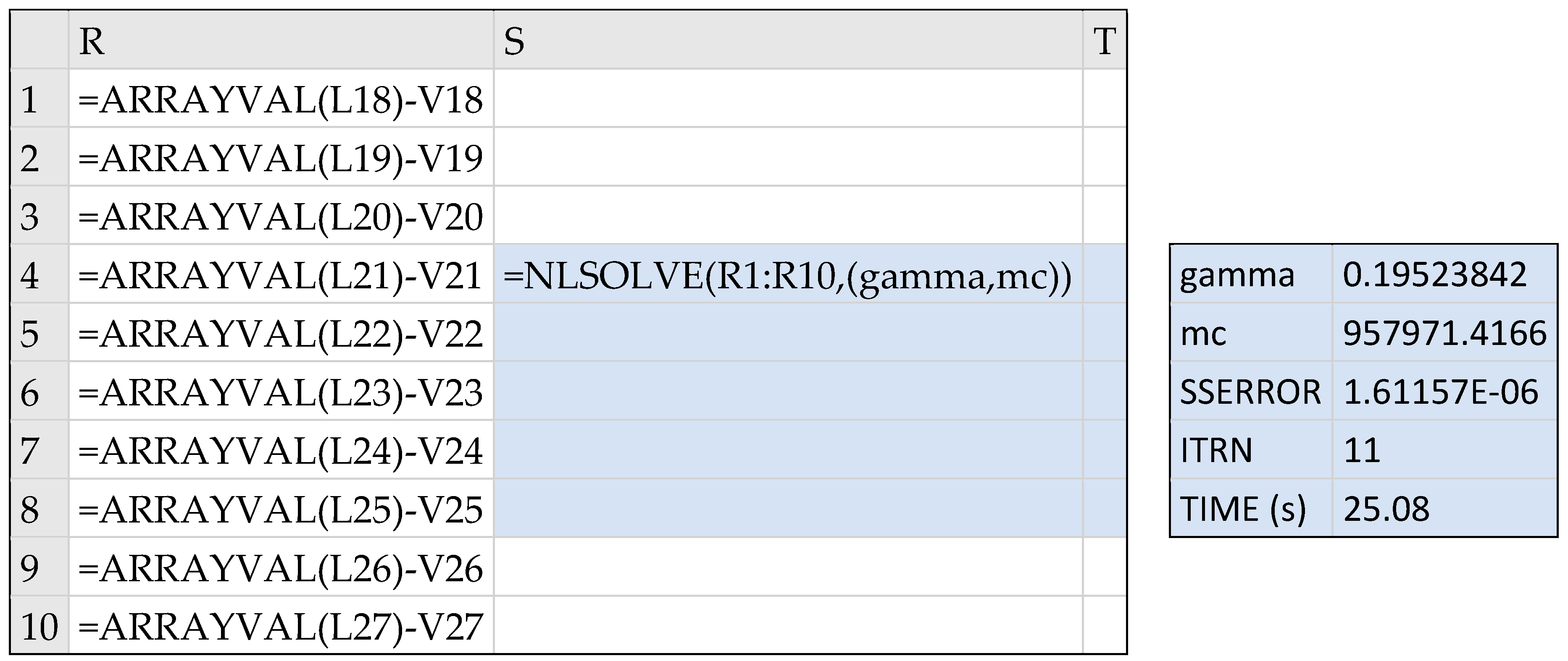
Using NLSOLVE differs from Excel NLP solver in multiple respects. First, unlike Excel Solver, which requires an explicit objective formula, NLSOLVE requires the list of individual residual constraint formulas. NLSOLVE defines the objective formula to be minimized implicitly as the sum of the squares of the residual constraint formulas which calculate the difference between selected values from PDASOLVE output solution array and corresponding target values. The residual constraint formula definitions for NLSOLVE are shown in column R of Figure 21. One additional requirement is that values from the PDASOLVE output array are referenced by the aid of a criterion function such as ARRAYVAL. A criterion function [22] simplifies defining complex constraints on computed values from the output, but for the purpose of this example, it is simply used to extract values from the output. Second, NLSOLVE is a pure spreadsheet function that is evaluated as an array formula in an allocated array by passing in the residual constraint formulas, and the design variables as shown in Formula (28)
=NLSOLVE(R1:R10, (gamma, mc))
We evaluated NLSOLVE Formula (28) in array S4:T8 as shown in Figure 21. It converged in about 25 s and displayed the results shown on the right of the Figure 21. The computed LM solution took less time and was slightly better, with a lower objective value of 1.611 × 10⁻⁶ from that obtained with Excel GRG solver. Since NLSOLVE is a pure spreadsheet function, it does not modify its arguments or update the spreadsheet calculation. Therefore, to update the PDASOLVE result, the computed numeric values for gamma and mc must be copied manually to their respective variable cells D6 and D7 of Figure 8.
7. Conclusions
We exploited the spreadsheet functional properties and Excel NLP solver command to devise a systematic method for modeling, solving, and optimizing general PDAE. The method is supported by a PDAE solver pure spreadsheet function design that encapsulates MOL implementation, permitting its integration with Excel NLP solver as a standard built-in math function. An alternative spreadsheet solver function, based on the LM algorithm, has also been developed and demonstrated as a substitute to using Excel NLP solver.
As has been illustrated by the detailed examples, applying the method involves no more than defining a few formulas that closely parallel the original mathematical equations without the need for any programming. The method also presents additional research opportunities to be explored in future work. In particular, for attempting a direct solution method for optimal control problems of partial differential equations. Such a method has been demonstrated with remarkable success using an analogous solver for ordinary DAEs [24].
The spreadsheet functions, PDASOLVE, and NLSOLVE utilized in this work, as well as analogous ordinary DAE solvers are available in a lightweight calculus add-in library, ExceLab [22], which integrates seamlessly with MS Excel Spreadsheet.
Supplementary Materials
The following are available online at https://www.mdpi.com/2297-8747/23/3/39/s1.
Conflicts of Interest
The author of the manuscript is the founder of ExcelWorks LLC of Massachusetts, USA supplying the Excel calculus add-in, ExceLab [22], utilized in this study.
Appendix A. Spreadsheet Tips
- Naming spreadsheet variables (e.g., B1 as t) makes it easier to read the formulas and to spot errors. However, it is also recommended to restrict the scope of a named variable to the specific sheet it will be used on, and not the whole workbook. This prevents accidental interdependence between multiple problems on different sheets sharing same named variables. Defining and restricting the scope of named variables is done using the Name Manager in Excel.
- Excel gives precedence to the unary negation operator over the power operator ‘^’. For example, Excel evaluates the formula ‘=−X1^2′ as ‘=(−X1)^2′ when the intention may have been to do ‘-(X1^2)’ instead. A simple fix is to use parentheses or to use the POWER function instead of the operator ‘^’. When using the IF statement in a formula, it is also important to verify the formula always evaluates to a numeric value for all possible conditions. Otherwise, the formula may evaluate to a nonnumeric Boolean condition leading to solver error.
- PDASOLVE function is designed to operate in two modes: a silent mode where only standard spreadsheet errors are returned like #VALUE! and a verbose mode where the function may display informative error or warning message alert in a popup window. It is recommended to work in the verbose mode when modeling and solving a PDAE problem, but switch to the silent mode before running the NLP Solver. Switching between the two modes is triggered by evaluating the formula ‘=VERBOSE(TRUE)’ or ‘=VERBOSE(FALSE)’ in any cell in the workbook. This was not needed in the example of this paper but for other problems, it is possible the NLP Solver may wander into illegal input space before it recovers and adjusts its search. The silent mode blocks any occasional error alerts from the calculus functions. Switching to the silent mode is not required with the alternative NLSOLVE method.
References
- Ghaddar, C.K. Unconventional Calculus Spreadsheet Functions. World Academy of Science, Engineering and Technology, International Science Index 112. Int. J. Math. Comput. Phys. Electr. Comput. Eng. 2016, 10, 160–166. Available online: http://waset.org/publications/10004374 (accessed on 1 August 2018).
- Schittkowski, K. Numerical Data Fitting in Dynamical Systems: A Practical Introduction with Applications and Software; Springer: New York, NY, USA, 2002. [Google Scholar]
- Gieschke, R.; Serafin, D. Development of Innovative Drugs via Modeling with MATLAB: A Practical Guide; Springer: New York, NY, USA, 2014. [Google Scholar]
- Lasdon, L.S.; Waren, A.D.; Jain, A.; Ratner, M. Design and Testing of a Generalized Reduced Gradient Code for Nonlinear Programming. ACM Trans. Math. Softw. 1978, 4, 34–50. [Google Scholar] [CrossRef] [Green Version]
- Schiesser, W.E. The Numerical Method of Lines; Academic Press: San Diego, CA, USA, 1991. [Google Scholar]
- Lam, C.-Y.; Alan Koh, F.H. A Partial Differential Equation Solver for the Classroom. Int. J. Eng. Ed. 2006, 22, 868–875. [Google Scholar]
- Hagler, M. Spreadsheet Solution of Partial Differential Equations. IEEE Trans. Educ. 1987, 3, 130–134. [Google Scholar] [CrossRef]
- Fae’q, A.A. Solutions of Partial Differential Equations Using Excel. Pak. J. Appl. Sci. 2001, 1, 458–465. [Google Scholar]
- Olsthoorn, T.N. Groundwater Modelling: Calibration and the Use of Spreadsheets; Delft University Press: Delft, The Netherlands, 1998. [Google Scholar]
- Karahan, H. Unconditional stable explicit finite difference technique for the advection-diffusion equation using spreadsheets. Adv. Eng. Softw. 2007, 38, 80–86. [Google Scholar] [CrossRef]
- Karahan, H.; Ayvaz, M.T. Time-Dependent Groundwater Modelling Using Spreadsheets. Comput. Appl. Eng. Educ. 2005, 13, 192–199. [Google Scholar] [CrossRef]
- Karahan, H. Implicit finite difference techniques for the advection-diffusion equation using spreadsheets. Adv. Eng. Softw. 2006, 37, 601–608. [Google Scholar] [CrossRef]
- Bhattacharjya, R.K. Solving groundwater flow inverse problem using spreadsheet solver. J. Hydrol. Eng. 2011, 16, 472–477. [Google Scholar] [CrossRef]
- Karahan, H. Predicting Muskingum flood routing parameters using spreadsheets. Comput. Appl. Eng. Educ. 2012, 20, 280–286. [Google Scholar] [CrossRef]
- Ghaddar, C.K. Method, Apparatus, and Computer Program Product for Optimizing Parameterized Models Using Functional Paradigm of Spreadsheet Software. U.S. Patent 9,286,286, 15 March 2016. [Google Scholar]
- Ghaddar, C.K. Method, Apparatus, and Computer Program Product for Solving Equation System Models Using Spreadsheet Software. U.S. Patent 9,892,108, 13 February 2018. [Google Scholar]
- Ghaddar, C.K. Method, Apparatus, and Computer Program Product for Solving an Equation System Using Pure Spreadsheet Functions. USA Patent. to be Issued 2018, in press.
- Levenberg, K. A Method for the Solution of Certain Non-Linear Problems in Least Squares. Q. Appl. Math. 1944, 2, 164–168. [Google Scholar] [CrossRef]
- Marquardt, D. An Algorithm for Least-Squares Estimation of Nonlinear Parameters. SIAM J. Appl. Math. 1963, 11, 431–441. [Google Scholar] [CrossRef]
- Hairer, E.; Wanner, G. Solving Ordinary Differential Equations II: Stiff and Differential-Algebraic Problems; Springer: Berlin/Heidelberg, Germany, 1996. [Google Scholar]
- Ghaddar, C.K. Unlocking the Spreadsheet Utility for Calculus: A Pure Worksheet Solver for Differential Equations. Spreadsheets Educ. 2016, 9, 5. [Google Scholar]
- ExceLab Calculus Add-in for Excel and Reference Manual. Available online: https://excel-works.com (accessed on 1 August 2018).
- Madsen, N.K.; Sincovec, R.F. Software for Partial Differential Equations. In Numerical Methods for Differential Systems; Lapidus, L., Schiesser, W.E., Eds.; Academic Press: New York, NY, USA, 1976. [Google Scholar]
- Ghaddar, C.K. Novel Spreadsheet Direct Method for Optimal Control Problems. Math. Comput. Appl. 2018, 23, 6. [Google Scholar] [CrossRef]
Figure 1.
Flowchart for a mathematically pure spreadsheet solver function design that shields numerical procedure from model inputs and output results.
Figure 1.
Flowchart for a mathematically pure spreadsheet solver function design that shields numerical procedure from model inputs and output results.

Figure 2.
Output layout for partial differential algebraic equation solver function (PDASOLVE) solution for a system of two variables using the snapshot format. In the transient format, the order of t and x is swapped. The display of first and second derivative variables is optional.
Figure 2.
Output layout for partial differential algebraic equation solver function (PDASOLVE) solution for a system of two variables using the snapshot format. In the transient format, the order of t and x is swapped. The display of first and second derivative variables is optional.

Figure 3.
Spreadsheet model for PDE system (9) and (10). The colored ranges are inputs to PDASOLVE function.
Figure 3.
Spreadsheet model for PDE system (9) and (10). The colored ranges are inputs to PDASOLVE function.
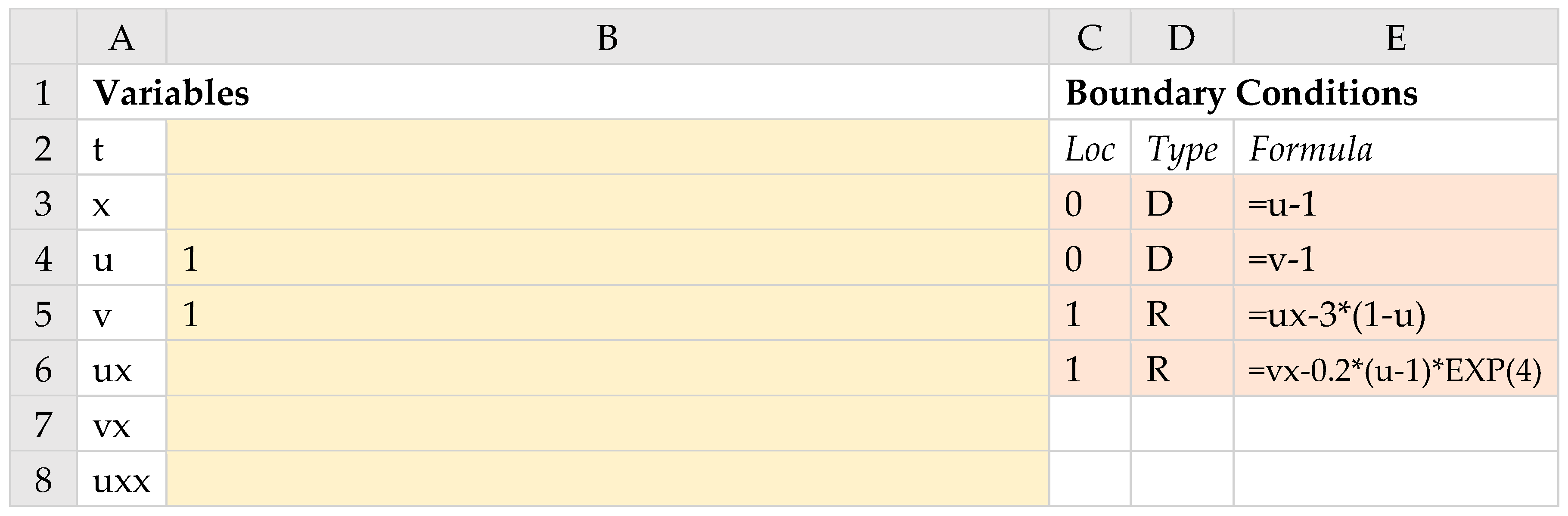

Figure 4.
Output PDE solution computed by Formula (13).
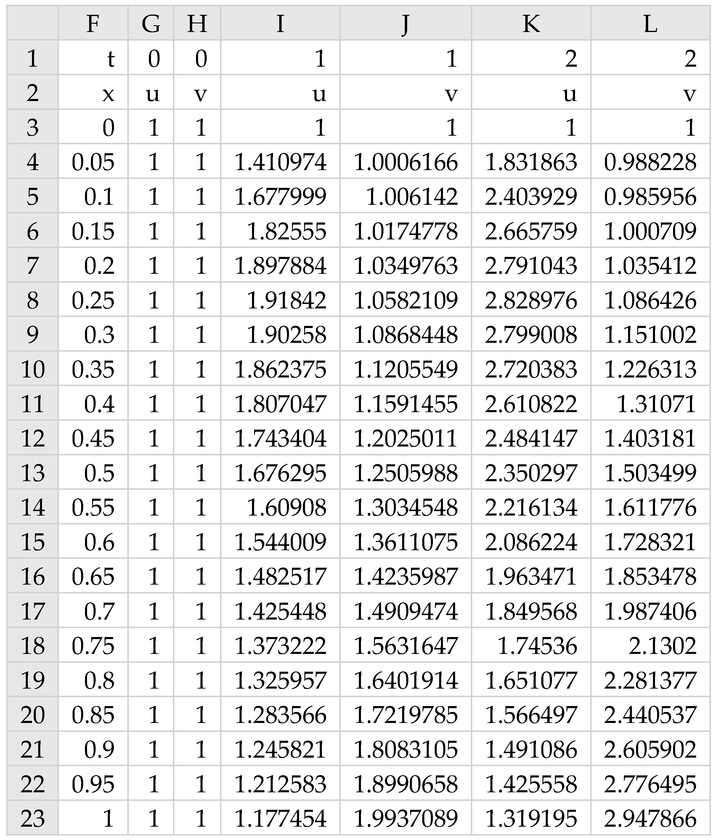

Figure 6.
Schematic of a battery model with three regions and three variables with initial conditions.
Figure 6.
Schematic of a battery model with three regions and three variables with initial conditions.

Figure 7.
Observed transient values for at .
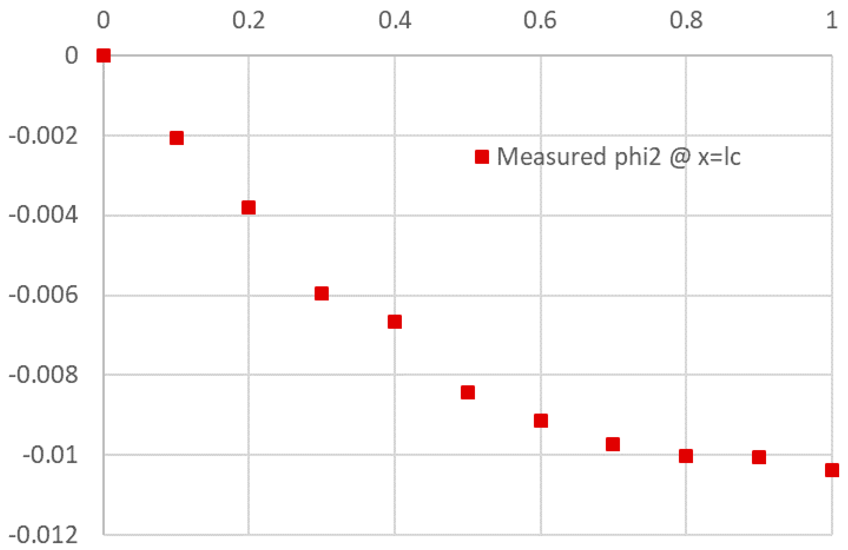
Figure 8.
Spreadsheet model for System (14)–(16) excluding boundary conditions. The colored ranges are inputs to PDASOLVE function.
Figure 8.
Spreadsheet model for System (14)–(16) excluding boundary conditions. The colored ranges are inputs to PDASOLVE function.

Figure 9.
Definition of boundary conditions listed in Table 4. The colored range is input to PDASOLVE function.
Figure 9.
Definition of boundary conditions listed in Table 4. The colored range is input to PDASOLVE function.

Figure 10.
Output solution computed by Formula (22).
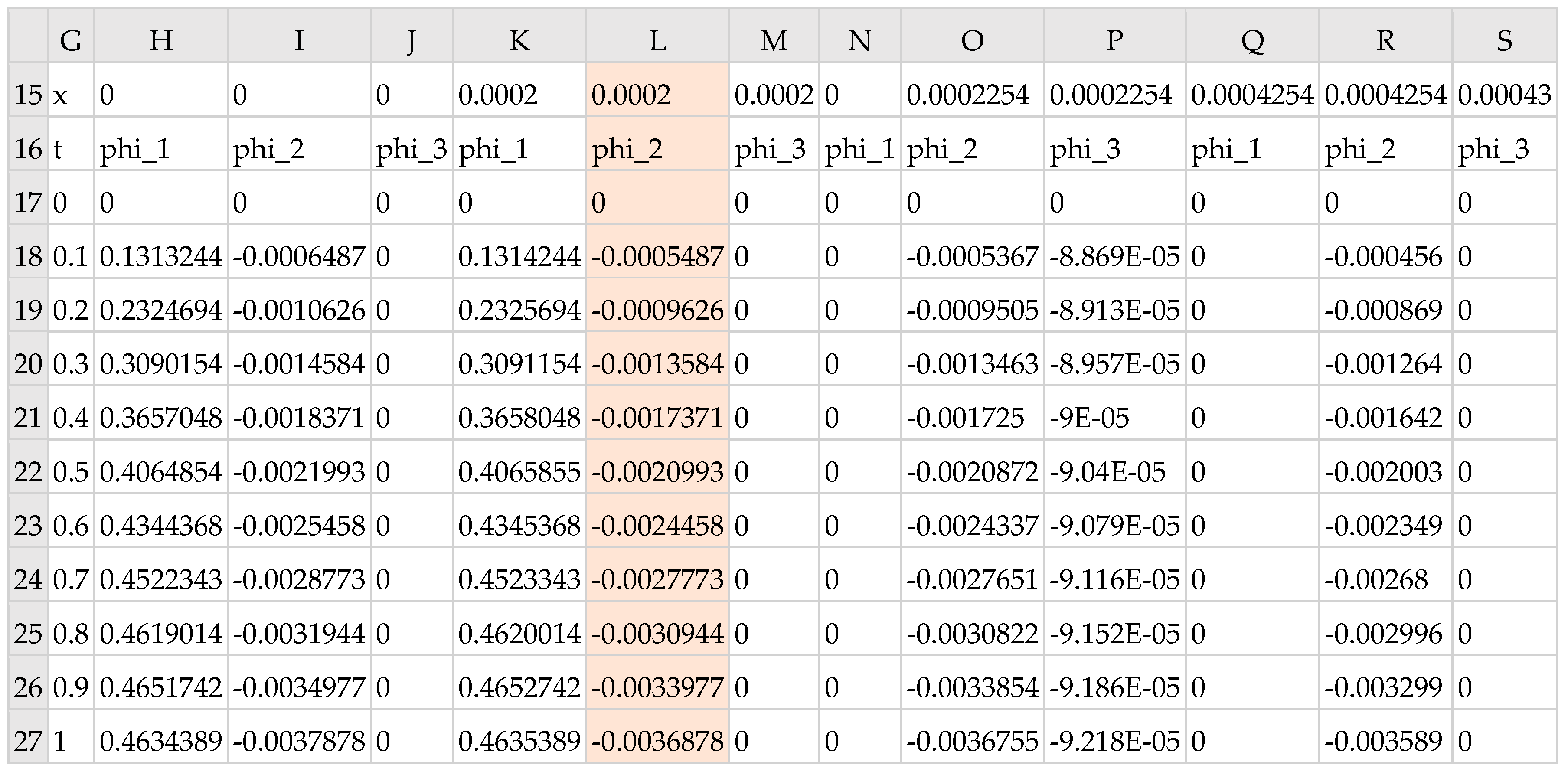
Figure 11.
A plot of computed and observed values for phi_2 at x = lc.

Figure 12.
Definitions for optional arguments to PDASOLVE function used in Formula (23).

Figure 13.
Partial listing of the output solution computed by Formula (23). The values for phi2x around x = ls are marked. phi2x is undefined at x = ls.
Figure 13.
Partial listing of the output solution computed by Formula (23). The values for phi2x around x = ls are marked. phi2x is undefined at x = ls.

Figure 14.
Definition of the objective formula, S2, to be minimized. Shown also is its initial value.
Figure 14.
Definition of the objective formula, S2, to be minimized. Shown also is its initial value.

Figure 15.
Excel Nonlinear Programming (NLP) solver dialog configured for problem (24).
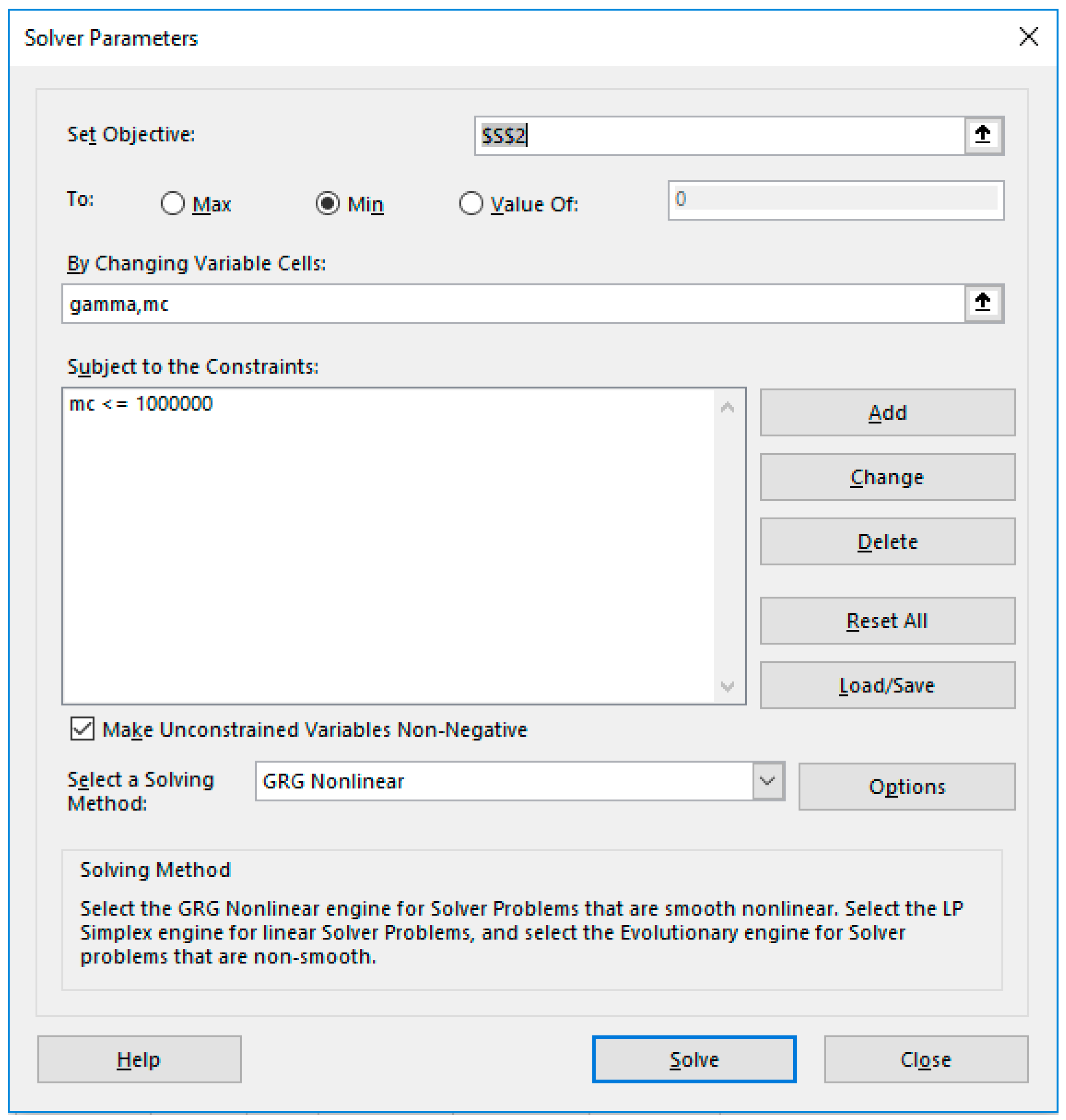
Figure 16.
Answer Report generated by Excel NLP solver as configured in Figure 15.
Figure 16.
Answer Report generated by Excel NLP solver as configured in Figure 15.

Figure 17.
Updated phi2 plot using optimal parameter values shown in Figure 16.
Figure 17.
Updated phi2 plot using optimal parameter values shown in Figure 16.
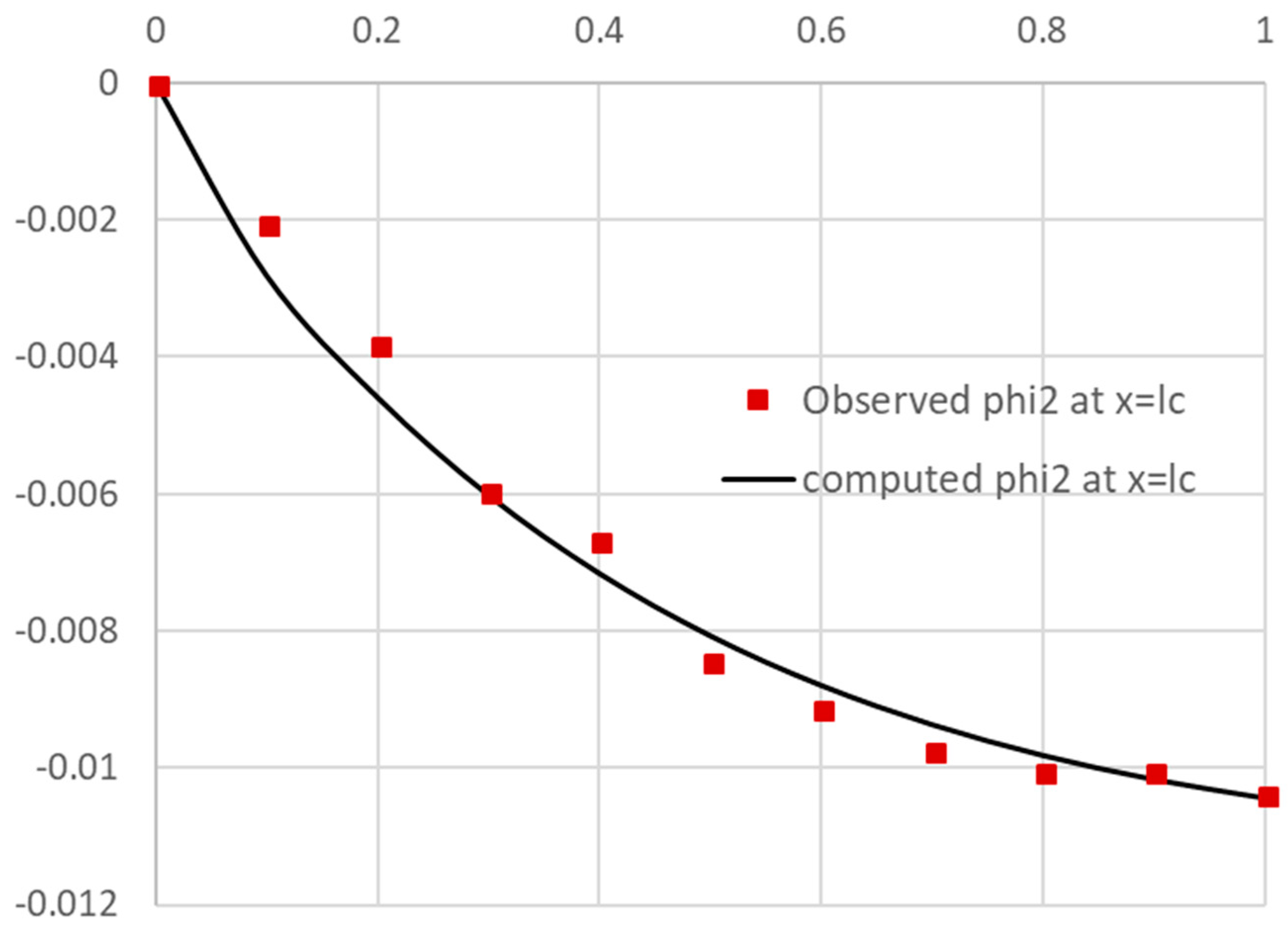
Figure 18.
Answer Report generated by Excel NLP solver by varying mc only while gamma was held constant.
Figure 18.
Answer Report generated by Excel NLP solver by varying mc only while gamma was held constant.

Figure 19.
Less than optimal solution obtained by estimating mc alone, while gamma was held constant.
Figure 19.
Less than optimal solution obtained by estimating mc alone, while gamma was held constant.

Figure 20.
Answer Report generated by Excel NLP solver for experiment of Section 5.2.
Figure 20.
Answer Report generated by Excel NLP solver for experiment of Section 5.2.

Figure 21.
Constraints formulas calculating the residuals between computed values of phi2 in Figure 10 and observed values stored in range V18:V27. The formulas and the design parameters are input to NLSOLVE function, which computes the optimal solution shown on right.
Figure 21.
Constraints formulas calculating the residuals between computed values of phi2 in Figure 10 and observed values stored in range V18:V27. The formulas and the design parameters are input to NLSOLVE function, which computes the optimal solution shown on right.


Table 1.
Definitions for domains, initial and boundary conditions for partial differential equations (PDE) (9) and (10).
Table 1.
Definitions for domains, initial and boundary conditions for partial differential equations (PDE) (9) and (10).
| Time Interval | |
| Spatial Domain | |
| Initial Values | |
| Left Boundary Conditions | |
| Right Boundary Conditions |
Table 2.
Absolute errors between analytical and numerical values of u(x, t) and v(x, t).
| x | ∆u(x, 1) | ∆u(x, 1) | ∆u(x, 2) | ∆v(x, 2) |
|---|---|---|---|---|
| 0.05 | −0.00161 | 0.001883 | −0.01313 | 0.016772 |
| 0.1 | −0.00768 | 0.003858 | −0.06329 | 0.034044 |
| 0.15 | −0.00233 | 0.005022 | −0.01932 | 0.044291 |
| 0.2 | 0.000774 | 0.005024 | 0.006273 | 0.044588 |
| 0.25 | 0.001279 | 0.004289 | 0.010422 | 0.038574 |
| 0.3 | 0.001003 | 0.003155 | 0.008158 | 0.028998 |
| 0.35 | 0.000714 | 0.001945 | 0.005796 | 0.018687 |
| 0.4 | 0.000539 | 0.000855 | 0.00435 | 0.00929 |
| 0.45 | 0.000441 | −1.1 × 10⁻⁶ | 0.003543 | 0.001819 |
| 0.5 | 0.000381 | −0.0006 | 0.003056 | −0.0035 |
| 0.55 | 0.000338 | −0.00095 | 0.002701 | −0.00678 |
| 0.6 | 0.000299 | −0.00111 | 0.002391 | −0.00832 |
| 0.65 | 0.000261 | −0.0011 | 0.002086 | −0.00848 |
| 0.7 | 0.000222 | −0.00095 | 0.001773 | −0.00741 |
| 0.75 | 0.000181 | −0.00066 | 0.001446 | −0.0052 |
| 0.8 | 0.00014 | −0.00019 | 0.001118 | −0.00138 |
| 0.85 | 0.000106 | 0.000522 | 0.000849 | 0.004463 |
| 0.9 | 9.24 × 10⁻⁵ | 0.001689 | 0.000741 | 0.014098 |
| 0.95 | −6.1 × 10⁻⁵ | 0.003434 | −0.00051 | 0.028505 |
| 1.0 | 0.005702 | 0.006291 | 0.047117 | 0.052134 |
Table 3.
Initial conditions for the state variables of System (14)–(16), and numerical values for parameters.
Table 3.
Initial conditions for the state variables of System (14)–(16), and numerical values for parameters.
| Fixed Parameters | Design Parameters | Initial Conditions |
|---|---|---|
| 254 | ||
Table 4.
Boundary conditions for System (14)–(16).
Table 5.
Assigned names for selected spreadsheet ranges which represent input arguments to PDASOLVE function.
Table 5.
Assigned names for selected spreadsheet ranges which represent input arguments to PDASOLVE function.
| Excel Range | Assigned Name |
|---|---|
| B21:B23 | Eqns |
| B2:B12 | Vars |
| F:2:H9 | BCs |
| D14:E14 | xDom |
| D15:E15 | tDom |
| C10:E12 | M |
| C21:D23 | Rgns |
Table 6.
Computed ratios of phi2x just before and after x = lc and x = ls.
| t | Ratio at lc | Ratio at ls |
|---|---|---|
| 0.1 | 2.000009 | 0.501111 |
| 0.2 | 1.9999213 | 0.501085 |
| 0.3 | 1.9998514 | 0.50106 |
| 0.4 | 1.9997839 | 0.501037 |
| 0.5 | 1.9997196 | 0.501014 |
| 0.6 | 1.999658 | 0.500993 |
| 0.7 | 1.9995992 | 0.500973 |
| 0.8 | 1.9995428 | 0.500954 |
| 0.9 | 1.999489 | 0.500936 |
| 1 | 1.9994374 | 0.500918 |
© 2018 by the author. Licensee MDPI, Basel, Switzerland. This article is an open access article distributed under the terms and conditions of the Creative Commons Attribution (CC BY) license (http://creativecommons.org/licenses/by/4.0/).
Share and Cite
MDPI and ACS Style
Ghaddar, C.K. Rapid Modeling and Parameter Estimation of Partial Differential Algebraic Equations by a Functional Spreadsheet Paradigm. Math. Comput. Appl. 2018, 23, 39. https://doi.org/10.3390/mca23030039
AMA Style
Ghaddar CK. Rapid Modeling and Parameter Estimation of Partial Differential Algebraic Equations by a Functional Spreadsheet Paradigm. Mathematical and Computational Applications. 2018; 23(3):39. https://doi.org/10.3390/mca23030039
Chicago/Turabian StyleGhaddar, Chahid Kamel. 2018. "Rapid Modeling and Parameter Estimation of Partial Differential Algebraic Equations by a Functional Spreadsheet Paradigm" Mathematical and Computational Applications 23, no. 3: 39. https://doi.org/10.3390/mca23030039