Qualitative Analysis of a Dengue Fever Model

Abstract

In this paper, a deterministic mathematical model of the Dengue virus with a nonlinear incidence function in a population is presented and rigorously analysed. The model incorporates control measures at the aquatic and adult stages of the vector (mosquito). The stability of the system is analysed for the disease-free equilibrium and the existence of endemic equilibria under certain conditions. The local stability of the Dengue-free equilibrium is investigated via the threshold parameter (reproduction number) that was obtained using the next-generation matrix techniques. The Routh–Hurwitz criterion, along with Descartes’ rule of signs change, established the local asymptotically stability of the model whenever $R_0<1$ and was unstable otherwise. The comparison theorem was used to establish the global asymptomatically stability of the model.

1. Introduction

Dengue fever is one of the infectious diseases that has continued to be a subject of major concern to public health. It is a mosquito-borne viral infection, which is endemic in more than a hundred countries in the world [1,2,3], usually in the tropical and sub-tropical regions of the world [1,4,5]. In recent years, the transmission has increased, predominantly in the urban and semi-urban areas [1,4], where 50–390 million people worldwide per year are infected, leading to half a million hospitalizations [3,6,7], with an approximate 25,000 deaths [3,6,8].

The disease has been well-known clinically for over 200 hundred years, but the etiology of the disease was not discovered until 1944 [5,9]. It was first recognized in the Philippines in 1953 and in Thailand in 1955 [5,9,10]. The threat of the outbreak now exists in Europe, with its first local transmission reported in France and Croatia in 2010, other cases have occurred in Florida (USA) and Yunnan (province of China) in 2013 [1,4].

Dengue hemorrhagic fever is an infectious tropical disease that is caused by an infective agent called the Dengue virus, of the family Flaviviridae, which has four distinguished serotypes that are denoted by I, II, III, and IV [5,10]. The virus is transmitted to humans by the bites of Aedes mosquitoes (Aedes aegypti and A. albopictus are the principal transistors). The infection remains in mosquitos till death [5,9].

The Dengue infection causes a spectrum of illness in humans, ranging from clinically inapparent, to severe and fatal hemorrhagic disease [5,10]. The incubation period (time between infection and appearance of symptoms) is from 3–14 days, but often, it is 4–7 days [3,6,11], and is generally observed clearly in older children and adults [5]. Dengue fever is characterized by the sudden onset of fever, frontal headache, nausea, vomiting, and other symptoms.

The use of mathematics in explaining the epidemiology of Dengue fever has been extensively studied by many researchers over the years, notable among these studies by the following authors [2,5,6,9,11,12,13]. In this study, since Dengue fever is spread between two-interacting populations (human–vector), we have designed and analysed a mathematical compartmental model that considers the human population and the vector population (mosquito). We extended the earlier model [6] by incorporating a ‘standard force of infection’ with the proportion of antibodies that were produced by a human in response to the incidence of infection that was caused by mosquitos, and vice versa. Additionally, an extension of the work is to consider some of the control effects or precautionary measures of the vector in the absence of a vaccination. These measures include the Larvicides for the Aquatic stage of the vector, which prevents the vector from breeding; Naled; and Environmental Protection Agency (EPA)-registered insects’ repellants to prevent getting bitten against the adult stage of the vectors.

2. Formulation of the Model

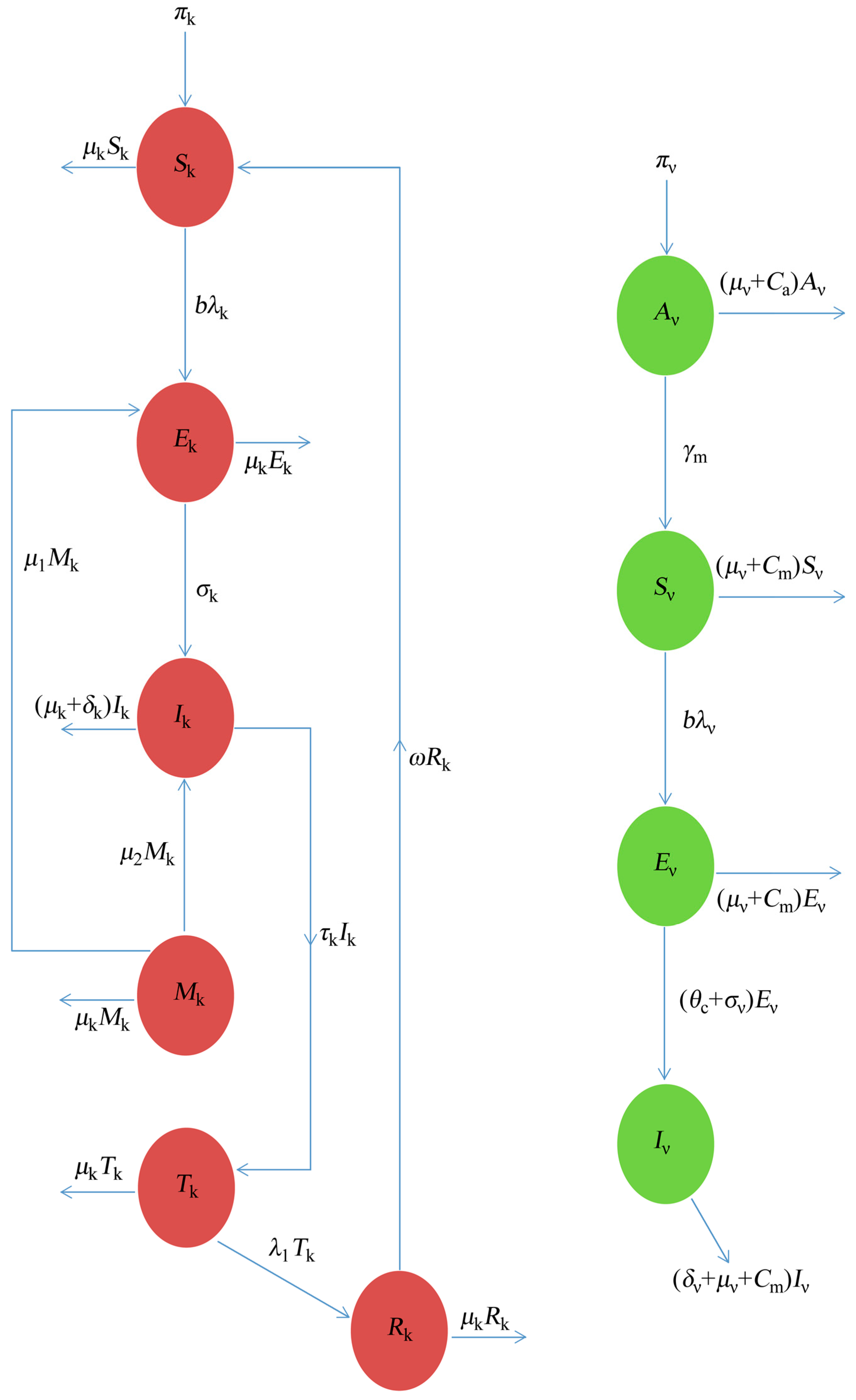
The formulation of the Dengue model requires the interaction between two-interacting populations (human–vector). The total human population at continuous-time t, denoted by $N_h\left(t\right)$, is subdivided into six compartments, namely: susceptible humans ($S_h$), exposed humans ($E_h$), infect humans ($I_h$), migrated population ($M_h$), treatment class ($T_h$), and recovered humans ($R_h$). Hence, the total human population $N_h\left(t\right)$ is given by the following:

$$N_h(t)=(S_h)+(E_h)+(I_h)+(M_h)+(T_h)+(R_h)$$

(1)

Similarly, the total vector population at continuous-time t, denoted by $N_{\nu }\left(t\right)$, is subdivided into four compartments, namely: aquatic class ($A_{\nu }$), susceptible mosquitoes ($S_{\nu }$), exposed mosquitoes ($E_{\nu }$), and infectious mosquitoes ($I_{\nu }$). Hence, the total vector population $N_{\nu }\left(t\right)$ is given by the following:

$$N_{\nu }(t)=(A_{\nu })+(S_{\nu })+(E_{\nu })+(I_{\nu })$$

(2)

The dynamics of the Dengue that are considered here, based on schematic illustration from Figure 1, is formulated and studied under the following assumption:

• The model assumes a homogeneous mixing of the human and vector (mosquito) populations, so that each mosquito bite has an equal chance of transmitting the virus to those that are susceptible in the population (or acquiring the infection from an infected human);
• Considering the saturated incidence rate (non-linear incidence), which incorporates the production of antibodies in response to the parasites causing Dengue in both the human and vector population (${\upsilon }_h,{\upsilon }_{\nu }$) respectively.
• The model considers the vector-aquatic class so as to investigate the effect of the control strategies, such as Larvicides at the aquatic stage;
• That the infectious mosquitoes remain infectious until death;
• There is a loss of immunity for the recovered human population; and
• Incorporating the controlling rate parameters, which will monitor the effects of control strategies at the aquatic stage ($A_{\nu }$) and adult stages ($S_{\nu },E_{\nu },I_{\nu }$).

In summary, following the assumptions from above, the transmission dynamics of Dengue in a population is given by the ten compartmental systems of the non-linear differential equation below, as follows:

$$\begin{array}{l}{\dot{S}}_h(t)={\pi }_h-\frac{b{\beta }_{h\nu }{S}_h(t)I_{\nu }(t)}{1+{\upsilon }_h{I}_{\nu }(t)}-{\mu }_h{S}_h(t)+\omega R_h(t)\\ \\ {\dot{E}}_h(t)=\frac{b{\beta }_{h\nu }{S}_h(t)I_{\nu }(t)}{1+{\upsilon }_h{I}_{\nu }(t)}+{\mu }_1{M}_h(t)-\left({\mu }_h+{\sigma }_h\right)E_h(t)\\ \\ {\dot{I}}_h(t)={\sigma }_h{E}_h(t)+{\mu }_2{M}_h(t)-\left({\mu }_h+{\tau }_h+{\delta }_h\right)I_h(t)\\ \\ {\dot{M}}_h(t)={\pi }_{mh}-\left({\mu }_1+{\mu }_2+{\mu }_h\right)M_h(t)\\ \\ {\dot{T}}_h(t)={\tau }_h{I}_h(t)-\left({\mu }_h+{\gamma }_1\right)T_h(t)\\ \\ {\dot{R}}_h(t)={\gamma }_1{T}_h(t)-{\mu }_h{R}_h(t)-\omega R_h(t)\\ \\ {\dot{A}}_{\nu }(t)={\pi }_{\nu }-\left({\gamma }_m+{\mu }_{\nu }+C_a\right)A_{\nu }(t)\\ \\ {\dot{S}}_{\nu }(t)={\gamma }_m{A}_{\nu }(t)-\frac{b{\beta }_{\nu h}{S}_{\nu }(t)I_h(t)}{1+{\upsilon }_{\nu }{I}_h(t)}-\left({\mu }_{\nu }+C_m\right)S_{\nu }(t)\\ \\ {\dot{E}}_{\nu }(t)=\frac{b{\beta }_{\nu h}{S}_{\nu }(t)I_h(t)}{1+{\upsilon }_{\nu }{I}_h(t)}-\left({\theta }_c+{\sigma }_{\nu }+{\mu }_{\nu }+C_m\right)E_{\nu }(t)\\ \\ {\dot{I}}_{\nu }(t)=\left({\theta }_c+{\sigma }_{\nu }\right)E_{\nu }(t)-\left({\delta }_{\nu }+{\mu }_{\nu }+C_m\right)I_{\nu }(t)\end{array}\}$$

(3)

where a dot is representing the differentiation with respect to time.

2.1. Analysis of the Model

Exploring the basic dynamical feature of the model is a necessity. For the Dengue model, Equation (3), which has been formulated above to be epidemiologically meaningful, it is very important to prove that all of the states variables are non-negative all of the time (t). In other words, the solution of the model, Equation (3), with positive initial values of data will remain positive at all times t ≥ 0.

Positivity and Boundedness of Solutions

Since the Dengue model, Equation (3), describes the interaction between the human and vector population, it is important to state that all of the parameters and variables that are involved are non-negative with respect to time. The Dengue model, Equation (3), will be considered in the biologically-feasible region $\mathrm{\Omega }={\mathrm{\Omega }}_h\times {\mathrm{\Omega }}_{\nu }\subset {\Re }_{+}^6\times {\Re }_{+}^4$, with the following:

$${\mathrm{\Omega }}_h=\left\{S_h,E_h,I_h,M_h,T_h,R_h\in {\Re }_{+}^6:N_h\le \frac{{\pi }_h}{{\mu }_h}\right\}$$

(4)

and

$${\mathrm{\Omega }}_{\nu }=\left\{A_{\nu },S_{\nu },E_{\nu },I_{\nu }\in {\Re }_{+}^4:N_{\nu }\le \frac{{\pi }_{\nu }}{{\mu }_{\nu }}\right\}$$

(5)

It can be shown that the set $\mathrm{\Omega }$ is a positively invariant set and the global attractor of this system. This implies that any phase trajectory that is initiated anywhere in the non-negative region ${\Re }_{+}^{10}$ of the phase space eventually enters the feasible region $\mathrm{\Omega }$ and remains in $\mathrm{\Omega }$ thereafter.

Lemma 1.

The region $\mathrm{\Omega }=\left\{S_h,E_h,I_h,M_h,T_h,R_h,A_{\nu },S_{\nu },E_{\nu },I_{\nu }\in {\Re }_{+}^{10}:N_h\le \frac{{\pi }_h}{{\mu }_h},N_{\nu }\le \frac{{\pi }_{\nu }}{{\mu }_{\nu }}\right\}$ is positively-invariant for the Dengue model, Equation (3).

Proof. 

The rate of change of the human total population is given by the following [14]:

$$\frac{d{N}_h}{dt}={\pi }_h-{\mu }_h{N}_h-{\delta }_h{I}_h+{\pi }_{mh}$$

(6)

and

$$\frac{d{N}_{\nu }}{dt}={\pi }_{\nu }-{\mu }_{\nu }{N}_{\nu }-C_a{A}_{\nu }-C_m\left(S_{\nu }+E_{\nu }+I_{\nu }\right)-{\delta }_{\nu }{I}_{\nu }$$

(7)

where $N_h=S_h+E_h+I_h+M_h+T_h+R_h$ and $N_{\nu }=A_{\nu }+S_{\nu }+E_{\nu }+I_{\nu }$.

Since $\frac{d{N}_h}{dt}\le {\pi }_h-{\mu }_h{N}_h+{\pi }_{mh}$ and $\frac{d{N}_{\nu }}{dt}\le {\pi }_{\nu }-{\mu }_{\nu }{N}_{\nu }$ for a special case ${\delta }_h={\delta }_{\nu }=C_a=C_m=0$, it follows that, whenever $N_h(t)>\frac{{\pi }_h+{\pi }_{mh}}{{\mu }_h}$ and $N_{\nu }(t)>\frac{{\pi }_{\nu }}{{\mu }_{\nu }}$, then $\frac{d{N}_h}{dt}<0$ and $\frac{d{N}_{\nu }}{dt}<0$, respectively.

Thus, since it follows from the right-hand side of Equations (6) and (7) that $\frac{d{N}_h}{dt}$ is bounded by ${\pi }_h-{\mu }_h+{\pi }_{mh}$ and $\frac{d{N}_{\nu }}{dt}$ is bounded by ${\pi }_{\nu }-{\mu }_{\nu }$, respectively, the standard comparison theorem [15] can be used to show the following:

$$N_h(t)\le N_h(0){\exp }^{-{\mu }_{h}t}+\frac{{\pi }_h+{\pi }_{mh}}{{\mu }_h}\left[1-{\exp }^{-{\mu }_{h}t}\right]\mathrm{if}{N}_h(0)\le \frac{{\pi }_h+{\pi }_{mh}}{{\mu }_h}$$

(8)

and

$$N_{\nu }(t)\le N_{\nu }(0){\exp }^{-{\mu }_{\nu }t}+\frac{{\pi }_{\nu }}{{\mu }_{\nu }}\left[1-{\exp }^{-{\mu }_{\nu }t}\right]\mathrm{if}{N}_{\nu }(0)\le \frac{{\pi }_{\nu }}{{\mu }_{\nu }}$$

(9)

Thus, $\mathrm{\Omega }$ is positively invariant under the flow that has been described by Equation (3), so that no solution path leaves through any boundary of $\mathrm{\Omega }$. Hence, in the region $\mathrm{\Omega }$, the Dengue model, Equation (3), is recognized to be mathematically and epidemiologically well-posed. Thus, it is sufficient to consider the dynamics of the model in the domain $\mathrm{\Omega }$. □

2.2. Stability of the Disease-Free Equilibrium (DFE)

The Dengue disease-free equilibrium is a point at which the population is free from Dengue fever. The disease-free equilibrium of the Dengue model, Equation (3), exists and is obtained by setting the right-hand side of the model system to zero, this is given by the following:

$$\begin{array}{cc}\hfill {\epsilon }_0& =\left\{S_h^{*},E_h^{*},I_h^{*},M_h^{*},T_h^{*},R_h^{*},A_{\nu }^{*},S_{\nu }^{*},E_{\nu }^{*},I_{\nu }^{*}\right\}\hfill \\ & =\left\{\frac{{\pi }_h}{{\mu }_h},0,0,0,0,0,\frac{{\pi }_{\nu }}{({\gamma }_m+{\mu }_{\nu }+C_a)},\frac{{\gamma }_m{\pi }_{\nu }}{({\gamma }_m+{\mu }_{\nu }+C_a)({\mu }_{\nu }+C_m)},0,0\right\}\hfill \end{array}$$

(10)

The linear stability of ${\epsilon }_0$ is studied using the next generation operator technique [16,17] on the system, Equation (3). Using the notations in [17], it follows that the matrices $F$ and $V$, for the new infection terms (transmission) and the remaining transfer terms (transition), respectively, are given by the following:

$$\begin{gathered} F=\left(\begin{array}{cccccc}0& 0& 0& 0& 0& b{S}_h^{*}{\beta }_{h\nu }\\ 0& 0& 0& 0& 0& 0\\ 0& 0& 0& 0& 0& 0\\ 0& 0& 0& 0& 0& 0\\ 0& b{S}_{\nu }^{*}{\beta }_{\nu h}& 0& 0& 0& 0\\ 0& 0& 0& 0& 0& 0\end{array}\right) \\ \mathrm{and}V=\left(\begin{array}{cccccc}{\kappa }_1& 0& -{\mu }_1& 0& 0& b{S}_h^{*}{\beta }_{h\nu }\\ -{\sigma }_h& {\kappa }_2& -{\mu }_2& 0& 0& 0\\ 0& 0& {\kappa }_3& 0& 0& 0\\ 0& -{\tau }_h& 0& {\kappa }_4& 0& 0\\ 0& 0& 0& 0& {\kappa }_8& 0\\ 0& 0& 0& 0& -{\kappa }_9& {\kappa }_{10}\end{array}\right) \end{gathered}$$

(11)

where

$$\begin{array}{l}{\kappa }_1=({\mu }_h+{\sigma }_h),{\kappa }_2=({\mu }_h+{\tau }_h+{\delta }_h),{\kappa }_3=({\mu }_1+{\mu }_2+{\mu }_h),{\kappa }_4=({\mu }_h+{\gamma }_1),\\ {\kappa }_8=({\theta }_c+{\sigma }_{\nu }+{\mu }_{\nu }+C_m),{\kappa }_9=({\theta }_c+{\sigma }_{\nu }),\mathrm{and}{\kappa }_{10}=({\delta }_{\nu }+{\mu }_{\nu }+C_m).\end{array}$$

It follows that the basic reproduction number of the model, Equation (3), denoted by $R_0$, is given by $R_0=\rho (F{V}^{-1})$, where $\rho$ is the spectral radius (maximum eigenvalues) [15,18]. Hence,

$$R_0=\sqrt{\frac{b^2{S}_h^{*}{\beta }_{h\nu }{S}_{\nu }^{*}{\beta }_{\nu h}{\sigma }_h{\kappa }_9}{{\kappa }_1{\kappa }_2{\kappa }_8{\kappa }_{10}}}$$

So that

$$R_0=\sqrt{\frac{b^2{S}_h^{*}{\beta }_{h\nu }{S}_{\nu }^{*}{\beta }_{\nu h}{\sigma }_h({\sigma }_{\nu }+{\theta }_c)}{({\mu }_h+{\sigma }_h)({\mu }_h+{\tau }_h+{\delta }_h)({\theta }_c+{\sigma }_{\nu }+{\mu }_{\nu }+C_m)({\delta }_{\nu }+{\mu }_{\nu }+C_m)}}$$

Hence,

$$R_0=\sqrt{R_h{R}_{\nu }}$$

(12)

where

$$R_h=\frac{b{S}_h^{*}{\beta }_{h\nu }{\sigma }_h}{({\mu }_h+{\sigma }_h)({\mu }_h+{\tau }_h+{\delta }_h)}$$

(13)

and,

$$R_{\nu }=\frac{b{S}_{\nu }^{*}{\beta }_{\nu h}({\sigma }_{\nu }+{\theta }_c)}{({\theta }_c+{\sigma }_{\nu }+{\mu }_{\nu }+C_m)({\delta }_{\nu }+{\mu }_{\nu }+C_m)}$$

(14)

In Equation (13), $R_h=\frac{b{S}_h^{*}{\beta }_{h\nu }{\sigma }_h}{({\mu }_h+{\sigma }_h)({\mu }_h+{\tau }_h+{\delta }_h)}$ describes the number of humans that just one infectious vector infects over its expected infection period in a completely susceptible human population. Also, $\frac{{\sigma }_h}{({\mu }_h+{\sigma }_h)}$ is the probability that a human will survive the exposed state, to become infectious, while $\frac{1}{({\mu }_h+{\tau }_h+{\delta }_h)}$ is the average duration of the infectious period of a human.

In Equation (14), $R_{\nu }=\frac{b{S}_{\nu }^{*}{\beta }_{\nu h}({\sigma }_{\nu }+{\theta }_c)}{({\theta }_c+{\sigma }_{\nu }+{\mu }_{\nu }+C_m)({\delta }_{\nu }+{\mu }_{\nu }+C_m)}$ signifies the number of vectors that have been infected by one infectious human during the period of infectiousness in a completely susceptible vector population. Also, $\frac{({\sigma }_{\nu }+{\theta }_c)}{({\theta }_c+{\sigma }_{\nu }+{\mu }_{\nu }+C_m)}$ is the probability that a vector will survive the exposed state to become infectious, while $\frac{1}{({\delta }_{\nu }+{\mu }_{\nu }+C_m)}$ is the average duration of the infectious period of the vector. Hence, using Theorem 2 in [19], the following result is established.

Lemma 2.

The disease-free state ${\epsilon }_0$ of the Dengue model that has been considered is locally asymptotically stable if $R_0<1$, and unstable if $R_0>1$.

Proof. The Jacobian matrix of the system, Equation (3), which was evaluated at the disease-free equilibrium point ${\epsilon }_0$, is obtained as follows:

$$J({\epsilon }_0)=\left(\begin{array}{cccccccccc}{J}_{11}& 0& 0& 0& 0& J_{16}& 0& 0& 0& J_{1,10}\\ 0& J_{22}& 0& J_{24}& 0& 0& 0& 0& 0& J_{2,10}\\ 0& J_{32}& J_{33}& J_{34}& 0& 0& 0& 0& 0& 0\\ 0& 0& 0& J_{44}& 0& 0& 0& 0& 0& 0\\ 0& 0& J_{53}& 0& J_{55}& 0& 0& 0& 0& 0\\ 0& 0& 0& 0& J_{65}& J_{66}& 0& 0& 0& 0\\ 0& 0& 0& 0& 0& 0& J_{77}& 0& 0& 0\\ 0& 0& J_{83}& 0& 0& 0& J_{87}& J_{88}& 0& 0\\ 0& 0& J_{93}& 0& 0& 0& 0& 0& J_{99}& 0\\ 0& 0& 0& 0& 0& 0& 0& 0& J_{10,9}& J_{10,10}\end{array}\right)$$

(15)

where

$$\begin{array}{l}{J}_{11}=-{\mu }_h,J_{22}=-{\kappa }_1,J_{32}={\sigma }_h,J_{33}=-{\kappa }_2,J_{53}={\tau }_h,J_{2,10}=b{\beta }_{h\nu }{S}_h^{*},\\ J_{24}={\mu }_1,J_{34}={\mu }_2,J_{44}=-{\kappa }_3,J_{83}=-b{\beta }_{\nu h}{S}_{\nu }^{*},J_{93}=b{\beta }_{\nu h}{S}_{\nu }^{*},\\ J_{55}=-{\kappa }_4,J_{64}={\gamma }_1,J_{17}=\omega ,J_{66}=-{\kappa }_5,J_{77}=-{\kappa }_6,J_{87}={\gamma }_m,\\ J_{88}=-{\kappa }_7,J_{99}=-{\kappa }_8,J_{10,9}={\kappa }_9,J_{10,10}=-{\kappa }_{10},J_{1,10}=-b{\beta }_{h\nu }{S}_h^{*}\end{array}$$

From Equation (15), it is sufficient for us to show that all of the eigenvalues of $J({\epsilon }_0)$ are negative. The first and eighth columns contain only the diagonal terms, which form the two negative eigenvalues, $-{\mu }_h$ and $-({\mu }_h+C_m)$, so that the other eight eigenvalues can be obtained from the sub-matrix $J_1({\epsilon }_0)$, which is formed by excluding the first and eighth rows and columns of $J({\epsilon }_0)$. Hence, $J_1({\epsilon }_0)$ is written as follows:

$$J_1({\epsilon }_0)=\left(\begin{array}{cccccccc}{J}_{22}& 0& J_{24}& 0& 0& 0& 0& J_{2,10}\\ J_{32}& J_{33}& J_{34}& 0& 0& 0& 0& 0\\ 0& 0& J_{44}& 0& 0& 0& 0& 0\\ 0& J_{53}& 0& J_{55}& 0& 0& 0& 0\\ 0& 0& 0& J_{65}& J_{66}& 0& 0& 0\\ 0& 0& 0& 0& 0& J_{77}& 0& 0\\ 0& J_{93}& 0& 0& 0& 0& J_{99}& 0\\ 0& 0& 0& 0& 0& 0& J_{10,9}& J_{10,10}\end{array}\right)$$

(16)

In the same way, the fifth and sixth column of $J_1({\epsilon }_0)$ contain only the diagonal term, which forms negative eigenvalues, $-({\mu }_h+\omega )$ and $-({\gamma }_m+{\mu }_{\nu }+C_a)$. The remaining six eigenvalues can be obtained from the sub-matrix $J_2({\epsilon }_0)$ written as follows:

$$J_2({\epsilon }_0)=\left(\begin{array}{cccccc}{J}_{22}& 0& J_{44}& 0& 0& J_{2,10}\\ J_{32}& J_{33}& J_{34}& 0& 0& 0\\ 0& 0& J_{44}& 0& 0& 0\\ 0& J_{53}& 0& J_{55}& 0& 0\\ 0& J_{93}& 0& 0& J_{99}& 0\\ 0& 0& 0& 0& J_{10,9}& J_{10,10}\end{array}\right)$$

(17)

Using the same approach, the fourth column and third column of $J_2({\epsilon }_0)$ contains only the diagonal term, which forms a negative eigenvalue, $-({\mu }_h+{\gamma }_1)$ and $-({\mu }_1+{\mu }_2+{\mu }_h)$. The remaining four eigenvalues can now be obtained by the characteristics equation of the sub-matrix $J_3({\epsilon }_0)$ written as follows:

$$J_3({\epsilon }_0)=\left(\begin{array}{cccc}-({\mu }_h+{\sigma }_h)& 0& 0& b{\beta }_{h\nu }{S}_h^{*}\\ {\sigma }_h& -({\mu }_h+{\tau }_h+{\delta }_h)& 0& 0\\ 0& b{\beta }_{\nu h}{S}_{\nu }^{*}& -({\theta }_c+{\sigma }_{\nu }+{\mu }_{\nu }+C_m)& 0\\ 0& 0& ({\theta }_c+{\sigma }_{\nu })& -({\mu }_{\nu }+{\delta }_{\nu }+C_m)\end{array}\right)$$

(18)

Hence, the eigenvalues of the matrix $J_3({\epsilon }_0)$ are the roots of the characteristics equation, as follows:

$$\begin{array}{l}(\lambda +{\mu }_h+{\sigma }_h)(\lambda +{\mu }_h+{\tau }_h+{\delta }_h)(\lambda +{\theta }_c+{\sigma }_{\nu }+{\mu }_{\nu }+C_m)\\ (\lambda +{\mu }_{\nu }+{\delta }_{\nu }+C_m)-b^2{\sigma }_{\nu }{\beta }_{h\nu }{S}_h^{*}{\beta }_{\nu h}{S}_{\nu }^{*}({\theta }_c+{\sigma }_{\nu })=0\end{array}$$

Let

$$\begin{array}{l}{\kappa }_1=({\mu }_h+{\sigma }_h),{\kappa }_2=({\mu }_h+{\tau }_h+{\delta }_h),\\ {\kappa }_8=({\theta }_c+{\sigma }_{\nu }+{\mu }_{\nu }+C_m),{\kappa }_{10}=({\mu }_{\nu }+{\delta }_{\nu }+C_m)\mathrm{and}{\kappa }_9=({\theta }_c+{\sigma }_{\nu })\end{array}$$

then, the equation above becomes the following:

$$B_4{\lambda }^4+B_3{\lambda }^3+B_2{\lambda }^2+B_1\lambda +B_0=0$$

(19)

where

$$\begin{array}{l}{B}_4=1\\ B_3={\kappa }_1+{\kappa }_2+{\kappa }_8+{\kappa }_{10}\\ B_2=({\kappa }_1+{\kappa }_2)({\kappa }_8+{\kappa }_{10})+{\kappa }_1{\kappa }_2+{\kappa }_8{\kappa }_{10}\\ B_1=({\kappa }_1+{\kappa }_2)({\kappa }_8{\kappa }_{10})+({\kappa }_8+{\kappa }_{10})({\kappa }_1{\kappa }_2)\\ B_0={\kappa }_1{\kappa }_2{\kappa }_8{\kappa }_{10}-b^2{\sigma }_{\nu }{\beta }_{h\nu }{S}_h^{*}{\beta }_{\nu h}{S}_{\nu }^{*}{\kappa }_9\end{array}\}$$

(20)

Further perturbation on $B_0$ in terms of the reproduction number, $R_0$ yields the following:

$$B_0={\kappa }_1{\kappa }_2{\kappa }_8{\kappa }_{10}(1-R_0^2)$$

(21)

We employ the Routh–Hurwitz criterion, [19], which states that all of the roots of the polynomial, Equation (19), have negative real parts if, and only if, the coefficients of $B_i$ are positive and matrices $H_i>0,$ for $i=0,1,2,3,4$ from (20), it is easy to see that $B_1>0,B_2>0,B_3>0,B_4>0,$ since all of the $B_i$ are positive. Moreover, if $R_0<0,$ it then follows from Equation (21) that $B_0>0.$ Also, the Hurwitz matrices for the polynomial Equation (19) are found to be positive. That is, $H_1=B_3>0,$ $H_2=\left|\begin{array}{cc}{B}_3& B_4\\ B_1& B_2\end{array}\right|>0,$ $H_3=\left|\begin{array}{ccc}{B}_3& B_4& B_0\\ B_1& B_2& B_3\\ 0& B_0& B_1\end{array}\right|>0$ and $H_4=\left|\begin{array}{cccc}{B}_3& B_4& 0& 0\\ B_1& B_2& B_3& B_4\\ 0& B_0& B_1& B_2\\ 0& 0& 0& B_0\end{array}\right|>0$. Hence, all of the eigenvalues of the Jacobian matrix $J({\epsilon }_0)$ have negative real parts whenever $R_0<1,$ and the disease-free equilibrium point is said to be locally asymptotically stable. However, if $R_0>1$, we deduce that $B_0<0$, and by Descartes’ rule of signs [19,20], there exists exactly one sign change in the sequence $B_4,B_3,B_2,B_1,B_0$ of the coefficients of the polynomial (19). So, there is one eigenvalue with a non-negative real part and hence, the disease-free equilibrium point is said to be unstable, which proclaims an existence of an endemic state of equilibria. □

2.3. The Existence of Stability Equilibrium Point

More than the existence of the disease-free equilibrium point, it is important to show that the model, Equation (3), has an endemic equilibrium point ${\epsilon }_1$. This is a positive steady solution where the disease persists in the population.

Theorem 1.

The Dengue model, Equation (3), has no endemic equilibrium when $R_0<1$ and a unique endemic equilibrium exists whenever $R_0>1.$

Proof. 

Let ${\epsilon }_1=\left\{S_h^{**},E_h^{**},I_h^{**},M_h^{**},T_h^{**},R_h^{**},A_{\nu }^{**},S_{\nu }^{**},E_{\nu }^{**},I_{\nu }^{**}\right\}$ be a non-trivial equilibrium of the model, Equation (3), such that all of the components of ${\epsilon }_1$ are non-negative.

Setting the right-hand sides of the system of equations in Equation (3) to zero and solving in terms of the associated form of infection at a steady-state for the state variables of the model yieldsthe following:

$$\begin{array}{l}{S}_h^{**}=\frac{{\pi }_h{\kappa }_4{\kappa }_5+\omega {\gamma }_1{\tau }_h{I}_h^{**}}{{\kappa }_4{\kappa }_5(b{\lambda }_h^{**}+{\mu }_h)},A_{\nu }^{**}=\frac{{\pi }_{\nu }}{{\kappa }_6},\\ \\ E_h^{**}=\frac{b{\lambda }_h^{**}{S}_h^{**}{\kappa }_3+{\mu }_1{\pi }_{mh}}{{\kappa }_1{\kappa }_3},S_{\nu }^{**}=\frac{{\pi }_{\nu }{\gamma }_m}{{\kappa }_6(b{\lambda }_{\nu }^{**}+{\kappa }_7)},\\ \\ M_h^{**}=\frac{{\pi }_{mh}}{{\kappa }_3},E_{\nu }^{**}=\frac{b{\lambda }_{\nu }^{**}{\pi }_{\nu }{\gamma }_m}{{\kappa }_6{\kappa }_8(b{\lambda }_{\nu }^{**}+{\kappa }_7)},\\ \\ T_h^{**}=\frac{{\tau }_h{I}_h^{**}}{{\kappa }_4},I_{\nu }^{**}=\frac{b{\lambda }_{\nu }^{**}{\pi }_{\nu }{\gamma }_m{\kappa }_9}{{\kappa }_6{\kappa }_8{\kappa }_{10}(b{\lambda }_{\nu }^{**}+{\kappa }_7)},\\ \\ R_h^{**}=\frac{{\gamma }_1{\tau }_h{I}_h^{**}}{{\kappa }_4{\kappa }_5},I_h^{**}=\frac{{\sigma }_{h}b{\lambda }_h^{**}{S}_h^{**}{\kappa }_3+{\sigma }_h{\mu }_1{\pi }_{mh}+{\kappa }_1{\mu }_2{\pi }_{mh}}{{\kappa }_1{\kappa }_2{\kappa }_3}\end{array}\}$$

Looking at the behavior of the solutions, it is not enough to stop there, but to test for the certainty of the solution. Hence, using the two force of infection

Table 1. Description of the parameters of the Dengue model, Equation (3).

Parameters	Description
${\pi }_h,{\pi }_{\nu }$	Recruitment rate of humans and vector, respectively
${\pi }_{mh}$	Recruitment rate of migrated population
${\beta }_{h\nu }$	Transmission rate from host to vector
${\beta }_{\nu h}$	Transmission rate from vector to host
$b$	The biting rate of vector
${\upsilon }_h$	The proportion of antibody produced by a human in response to the incidence of infection caused by the vector
${\upsilon }_{\nu }$	The proportion of antibody produced by a vector in the response to the incidence of infection caused by the human
${\mu }_h,{\mu }_{\nu }$	The natural death rate of humans and vector, respectively
${\mu }_1,{\mu }_2$	Transition rates between exposed humans and infectious humans
${\sigma }_h$	Progression rate of exposed humans to infectious class
${\sigma }_{\nu }$	Progression rate of the exposed vector to the infectious class
${\tau }_h$	Treatment rate of the infectious individuals
$\omega$	Per capita rate of loss of immunity in humans
${\gamma }_1$	Recovery rate due to treatment
${\gamma }_m$	Mean aquatic transition rate
${\delta }_h,{\delta }_{\nu }$	Disease—an induced death rate of humans and vector, respectively
$C_a,C_m$	Control effect rate
${\theta }_c$	Extrinsic incubation rate of vector

, as follows:

$${\lambda }_h^{**}=\frac{{\beta }_{h\nu }{I}_{\nu }^{**}}{1+{\upsilon }_h{I}_{\nu }^{**}}\mathrm{and}{\lambda }_{\nu }^{**}=\frac{{\beta }_{\nu h}{I}_h^{**}}{1+{\upsilon }_{\nu }{I}_h^{**}}$$

(22)

The endemic equilibria of the model, Equation (3), satisfies the following polynomial perturbing the two forces of infection together:

$$P_1{({\lambda }_h^{**})}^2+P_2({\lambda }_h^{**})-P_3=0$$

(23)

where

$$\begin{array}{l}{P}_1={\upsilon }_{\nu }b{S}_h^{**}{\kappa }_3{\sigma }_h\\ P_2={\upsilon }_{\nu }{\sigma }_h{\mu }_1{\pi }_{mh}+{\upsilon }_{\nu }{\kappa }_1{\mu }_2{\pi }_{mh}+{\kappa }_1{\kappa }_2{\kappa }_3-b^2{\beta }_{h\nu }{S}_h^{**}{S}_{\nu }^{**}{\kappa }_9{\kappa }_3{\sigma }_h\\ P_3=b{\beta }_{h\nu }{S}_{\nu }^{**}{\kappa }_9({\sigma }_h{\mu }_1{\pi }_{mh}+{\kappa }_1{\mu }_2{\pi }_{mh})\end{array}$$

(24)

According to the Routh–Hurwitz criterion, if we observe Equation (24), then there exists only one sign change, thus there is only one real root that exists for the equation. Therefore, the system, Equation (3), has a unique endemic equilibrium point of the form ${\epsilon }_1=\left\{S_h^{**},E_h^{**},I_h^{**},M_h^{**},T_h^{**},R_h^{**},A_{\nu }^{**},S_{\nu }^{**},E_{\nu }^{**},I_{\nu }^{**}\right\}$, which has been presented in Equation (24), above. □

So we claim the following:

Lemma 3.

The model, Equation (3), has one positive (endemic) equilibrium whenever $R_0>1,$ and no positive equilibrium (endemic) outbreak of disease at $R_0<1.$

Hence, the above endemic equilibrium state analysis shows that the basic Dengue model, Equation (3), has a global asymptotically stable disease-free equilibrium whenever $R_0<1$, and a unique endemic equilibrium if $R_0>1$.

2.4. Global Asymptotic Stability of the Disease-Free Equilibrium Point

We employed the theorem by Carlos Castillo-Chavez [21] in order to investigate the global asymptotical stability of the Dengue model, Equation (3). Re-writing the model, Equation (3), as follows:

$$\begin{array}{l}\frac{dX}{dt}=F(X,I),\\ \frac{dI}{dt}=G(X,I),G(X,I)=0\end{array}$$

(25)

where $X=(S_h,R_h,A_{\nu },S_{\nu })$ and $I=(E_h,I_h,M_h,T_h,E_{\nu },I_{\nu })$, with the components of $X\in {\Re }^4$ denoting the uninfected population and the components of $I\in {\Re }^6$ denoting the infected population.

The disease-free equilibrium is denoted as follows:

$${\epsilon }_0=(X^{*},0),X^{*}=\left(\frac{{\pi }_h}{{\mu }_h},\frac{{\pi }_{\nu }}{({\gamma }_m+{\mu }_{\nu }+C_a)},\frac{{\gamma }_m{\pi }_{\nu }}{({\gamma }_m+{\mu }_{\nu }+C_a)({\mu }_{\nu }+C_m)}\right)$$

(26)

The conditions $(H1)$ and $(H2)$, in Equation (27) below, must be satisfied in order to guarantee a global asymptotic stability.

$(H1)$

$$\mathrm{For}\frac{dX}{dt}=F(X,0),X^{*}\mathrm{is}\mathrm{globally}\mathrm{asymptotically}\mathrm{stable}\left(\mathrm{GAS}\right)$$

$(H2)$

$$G(X,I)=AI-\widehat{G}(X,I),\widehat{G}(X,I)\ge 0(X,I)\in \mathrm{\Omega }$$

(27)

where $A=D_{I}G(X^{*},0)$ is an M-matrix (the off-diagonal elements of $A$ are nonnegative) and $\mathrm{\Omega }$ is the region where the model (3) makes biological sense.

If the system, Equation (25), satisfies the condition, Equation (27), above, then the following theorem holds:

Theorem 2.

The fixed point ${\epsilon }_0=(X^{*},0)$ is a globally asymptotically stable equilibrium of system, (25) provided that $R_0<1$ and that the assumptions in (27) are satisfied.

Proof. 

From the Dengue model, Equation (3), we have the following:

$$F(X,0)=\left(\begin{array}{c}{\pi }_h-{\mu }_h{S}_h\\ {\pi }_{\nu }-({\gamma }_m+{\mu }_{\nu }+C_a)A_{\nu }\\ {\gamma }_m{A}_{\nu }-({\mu }_{\nu }+C_m)S_{\nu }\end{array}\right)$$

(28)

and

$$A=\left(\begin{array}{cccccc}{k}_1& 0& {\mu }_1& 0& 0& b{\beta }_{h\nu }{S}_h^{*}\\ {\sigma }_h& k_2& {\mu }_2& 0& 0& 0\\ 0& 0& k_3& 0& 0& 0\\ 0& {\tau }_h& 0& k_4& 0& 0\\ 0& b{\beta }_{\nu h}{S}_{\nu }^{*}& 0& 0& k_5& 0\\ 0& 0& 0& 0& k_7& k_6\end{array}\right)$$

(29)

where

$$\begin{array}{l}{k}_1=-({\mu }_h+{\sigma }_h),k_2=-({\mu }_h+{\tau }_h+{\delta }_h),k_3=-({\mu }_1+{\mu }_2+{\mu }_h),k_4=-({\mu }_h+{\gamma }_1),\\ k_5=-({\theta }_c+{\sigma }_{\nu }+{\mu }_{\nu }+C_m),k_6=-({\delta }_{\nu }+{\mu }_{\nu }+C_m),k_7=({\theta }_c+{\sigma }_{\nu })\end{array}$$

(30)

By the condition, as follows, $(H2):$

$$\widehat{G}(X,I)=\left(\begin{array}{c}{\widehat{G}}_1(X,I)\\ {\widehat{G}}_2(X,I)\\ {\widehat{G}}_3(X,I)\\ {\widehat{G}}_4(X,I)\\ {\widehat{G}}_5(X,I)\\ {\widehat{G}}_6(X,I)\end{array}\right)=\left(\begin{array}{c}b{\beta }_{h\nu }{S}_h^{*}{I}_{\nu }\left(1-\frac{S_h}{S_h^{*}(1+{\upsilon }_h{I}_{\nu })}\right)\\ 0\\ 0\\ 0\\ b{\beta }_{\nu h}{S}_{\nu }^{*}{I}_h\left(1-\frac{S_{\nu }}{S_{\nu }^{*}(1+{\upsilon }_{\nu }{I}_h)}\right)\\ 0\end{array}\right)$$

Since $0\le S_h$ and $0\le S_{\nu }$, it is clear that $\widehat{G}(X,I)\ge 0.$ It is also clear that the disease-free point $X^{*}=\left(\frac{{\pi }_h}{{\mu }_h},\frac{{\pi }_{\nu }}{({\gamma }_m+{\mu }_{\nu }+C_a)},\frac{{\gamma }_m{\pi }_{\nu }}{({\gamma }_m+{\mu }_{\nu }+C_a)({\mu }_{\nu }+C_m)}\right)$ is a GAS equilibrium of $\frac{dX}{dt}=F(X,0).$ Hence, by the above theorem, the disease-free equilibrium ${\epsilon }_0=(X^{*},0)$ is globally asymptotically stable. □

3. Conclusions

A deterministic mathematical model of the Dengue virus with nonlinear incidence function in a population, with a consideration of some control measures (strategies) at the aquatic and adult stages of the vector (mosquito) Table 1, was presented and rigorously analysed. The disease-free equilibrium, represented by $({\epsilon }_0)$, was shown to be locally asymptotically stable, whenever the reproduction number $(R_0)$ was less than unity; additionally, the existence of the endemic equilibria state was analysed under certain conditions. The global asymptotically stability of the model was shown by the comparison theorem techniques, and the results showed that the disease-free equilibrium was globally asymptotically stable whenever the reproduction number $(R_0)$ was less than unity.

4. Further Research

Dengue fever is a health challenge disease that remains endemic, usually in the tropical and sub-tropical regions of the world. Hence, it is important to look into the re-occurrence of its outbreak by considering the backward bifurcation of the model that has been considered (because of the temporary immunity that is acquired by the recovered individuals), and the sensitivity analysis of the model, which tells the importance of each parameter to the disease transmission in the population.

References

- Bowman, C.; Gumel, A.B.; van den Driessche, P.; Wu, J.; Zhu, H. Mathematical Model for Assessing Control Strategies Against West Nile Virus. Bull. Math. Biol. 2005, 67, 1107–1133. [Google Scholar] [CrossRef] [PubMed]
- Garba, S.M.; Gumel, A.B.; Abu Bakar, M.R. Backward Bifurcations in Dengue Transmission Dynamics. Math. Biosci. 2008, 201, 11–25. [Google Scholar] [CrossRef] [PubMed] [Green Version]
- World Health Organization. Available online: http://www.who.int/Denguecontrol/faq/en/index6.html (accessed on 30 May 2018).
- Bakach, I. A Survey of Mathematical Model of Dengue Fever. Master’s Thesis, Georgia Southern University, Statesboro, GA, USA, 2015. [Google Scholar]
- Esteva, L.; Vargas, C. Coexistence of Different Serotypes of Dengue Virus. J. Math. Biol. 2003, 46, 31–47. [Google Scholar] [CrossRef] [PubMed]
- Hossain, M.S.; Nayeem, J.; Podder, C. Effects of migratory population and control strategies on the transmission dynamics of Dengue fever. J. Appl. Math. Bioinform. 2015, 5, 43–80. [Google Scholar]
- Wilder-Smith, A.; Schwartz, E. Dengue in travelers. N. Engl. J. Med. 2005, 353, 924–932. [Google Scholar] [CrossRef] [PubMed]
- Varatharaj, A. Encephalitis in the clinical spectrum of Dengue infection. Neurol. India 2010, 58, 585591. [Google Scholar] [CrossRef] [PubMed]
- Chowell, G.; Diaz-Duenas, P.; Miller, J.C.; Alcazar-Velazco, A.; Hyman, J.M.; Fenimore, P.W.; Castillo-Chavez, C. Estimation of the Reproduction Number of Dengue Fever from Spatial Epidemic Data. Math. Biosci. 2007, 208, 571–589. [Google Scholar] [CrossRef] [PubMed]
- Jelinek, T. Dengue Fever in International Travelers. Clin. Infect. Dis. 2000, 31, 144147. [Google Scholar] [CrossRef] [PubMed]
- Esteva, L.; Vargas, C. A Model for Dengue Disease with Variable Human Population. J. Math. Biol. 1999, 38, 220–240. [Google Scholar] [CrossRef] [PubMed]
- Coutinho, F.A.B.; Burattini, M.N.; Lopez, L.F.; Massad, E. Threshold Conditions for a Non-Autonomous Epidemic System Describing the Population Dynamics of Dengue. Bull. Math. Biol. 2006, 68, 2263–2282. [Google Scholar] [CrossRef] [PubMed]
- Esteva, L.; Vargas, C. Influence of Vertical and Mechanical Transmission on the Dynamics of Dengue Disease. Math. Biosci. 2000, 167, 51–64. [Google Scholar] [CrossRef]
- Oke, S.I.; Matadi, M.B.; Xulu, S.S. Optimal Control Analysis of a Mathematical Model for Breast Cancer. Math. Comput. Appl. 2018, 23, 21. [Google Scholar] [CrossRef]
- Akinpelu, F.O.; Ojo, M.M. A Mathematical Model for the Dynamic Spread of Infection Caused by Poverty and Prostitution in Nigeria. Int. J. Math. Phys. Sci. Res. 2016, 4, 33–47. [Google Scholar]
- Hethcote, H.W.; Thieme, H.R. Stability of the Endemic Equilibrium in Epidemic Models with Subpopulations. Math. Biosci. 1985, 75, 205–227. [Google Scholar] [CrossRef]
- Derouich, M.; Boutayeb, A. Dengue Fever: Mathematical Modelling and Computer Simulation. Appl. Math. Comput. 2006, 177, 528–544. [Google Scholar] [CrossRef]
- Bock, W.; Jayathunga, Y. Optimal control and basic reproduction numbers for a compartmental spatial multipatch dengue model. Math. Methods Appl. Sci. 2018, 41, 3231–3245. [Google Scholar] [CrossRef]
- Van den Driessche, P.; Watmough, J. Reproduction numbers and sub-threshold endemic equilibria for compartmental models of disease transmission. Math. Biosci. 2002, 180, 29–48. [Google Scholar] [CrossRef]
- Olaniyi, S.; Obabiyi, O.S. Mathematical model for malaria transmission dynamics in human and mosquito populations with nonlinear forces of infection. Int. J. Pure Appl. Math. 2013, 88, 125–156. [Google Scholar] [CrossRef]
- Castillo-Chavez, C.; Feng, Z.; Huang, W. On the Computation of Ro and Its Role on Global Stability. In Mathematical Approaches for Emerging and Reemerging Infectious Diseases: An Introduction; Springer: New York, NY, USA, 2002; pp. 229–250. [Google Scholar]
Figure 1.
The schematic illustration of the Dengue model.