Explicit Solutions for the (2 + 1)-Dimensional Jaulent–Miodek Equation Using the Integrating Factors Method in an Unbounded Domain


Department of Mathematics and Physics, Faculty of Engineering, Zagazig University, Zagazig, Egypt
*
Author to whom correspondence should be addressed.
Math. Comput. Appl. 2018, 23(1), 15; https://doi.org/10.3390/mca23010015
Submission received: 28 February 2018
/
Revised: 15 March 2018
/
Accepted: 16 March 2018
/
Published: 16 March 2018
Abstract
:In this work, we prove that the integrating factors can be used as a reduction method. Analytical solutions of the Jaulent–Miodek (JM) equation are obtained using integrating factors as an extension of a recent work where, through hidden symmetries, the JM was reduced to ordinary differential equations (ODEs). Some of these ODEs had no quadrature. We here derive several new solutions for these non-solvable ODEs.
1. Introduction
Nonlinear partial differential equations (NLPDEs) play an important role in various branches of scientific such as fluid mechanics, optical fibers, medical (breast cancer), oceans engineering, and other applications [1,2,3]. Analytical solutions for these equations are obtained using the homotopy perturbation method, Darboux transformation, variational iteration, Painlevé expansions, the homogeneous balance method, the Jacobi elliptic function, the exp-function method, and extended tanh-function [4,5,6,7,8,9,10,11,12,13]. The (2 + 1)-dimensional Jaulent–Miodek (JM) evolution equation is a highly nonlinear partial differential, previously solved analytically using several methods such as Hirota’s bilinear method [14], leading to a multiple-soliton solution of this equation.
Generalized solitary solution and generalized compacton-like solutions were also obtained using the exp-function method in [12] for the JM equation by introducing a new a complex variable that transforms the PDE to an ODE and then assumes the solution in the form of exponential terms with constants that are determined later. Applying the direct symmetry method in [15] leads to symmetry reductions and some new exact solutions of the JM equation. In [4], the Homotopy perturbation method was applied to solve the JM equation. In the JM equation [16], optimal hidden symmetries were detected, and the JM equation reduces to an ODE through these hidden symmetries. Some of the obtained ODEs were found to be non-integrable. This is where our work begins. We solve these equations using the Lie integrating factors.
The paper is constituted of five sections. In Section 2, an introduction to the Jaulent–Miodek equation is shown. In Section 3, the reduction of the JM equation to an ordinary differential equation (ODE) occurs in three steps. For each Lie vector, the following steps apply:
- The JM partial differential equation variables (x, y, t) are reduced to a PDE in two variables (r, s) whose Lie symmetries are evaluated.
- These symmetries are used for a further reduction of independent variables from (r, s) to one variable ().
- The resulting ODE non-solvable equations, through their corresponding Integrating Factors are reduced to new solvable ones.
2. Mathematical Model
The four JM models [1] have the following forms:
where w(x, y, t) is an analytic function with respect to the variables x, y, and t; the subscripts denote the partial derivatives and and .
We choose to work on Equation (1c) where we use the transformation to overcome the integral term. This leads to a fourth order differential equation:
An investigation of its Lie vectors using Maple results in eight Lie vectors:
3. Reduction of the Independent Variables in Jaulent–Miodek Equation (2)
In this paragraph, we will study, among the eight Lie vectors obtained in [16], only those vectors leading to ODEs with no quadrature.
3.1. Reduction of the JM Partial Differential, Equation (2), Using
The optimal vector reduces Equation (2) (where variable u is a dependent variable, and (x, y, t) are the independent variables) to a PDE of the form
where F is the new independent variable and . This equation has six Lie vectors:
Only is found to be a hidden symmetry [1] (Hidden symmetries are different from the original equation Lie vectors.). This vector is used to transform JM to a nonlinear fourth degree ordinary differential equation of the form
where In the original work [16], Equation (6) was solved using its hidden vectors through successive Lie reductions. We here will use the integrating factors and compare the results.
3.1.1. Integrating Factor Technique to Obtain an Explicit Solution
We first deduce Equation (6) Integrating Factors using Maple:
These Integrating Factors reduces Equation (6) to
This equation possesses symmetry vectors
These two vectors are used to reduce Equation (8) to a differential order.
Reductions of Equation (8)
Vector reduces Equation (8) to a first order, ordinary differential equation of the form
This equation has a closed-form solution:
Back-substituting for the variable and integrating Equation (11), we obtain
where , and c and are integration constants. Then, back-substituting, we obtain
where . Hence,
Back to the original variable , we obtain;
This result is different from the one obtained in [1]:
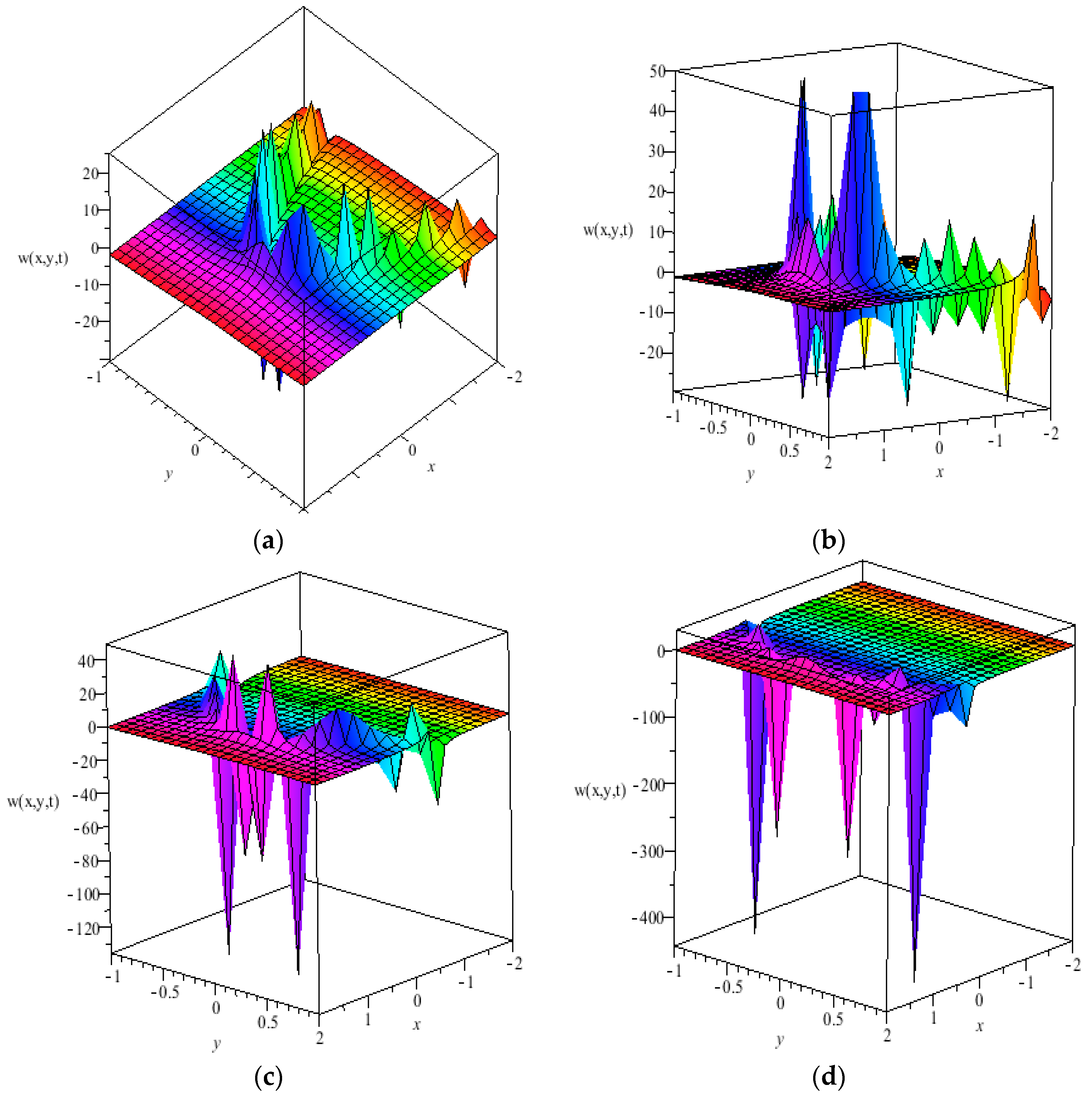
Our results are plotted in Figure 1a–d for different times: 03, 0.5, 0.8, and 1.2 s.
The previously results show that, with time marching, a parabolic middle peak upward advancing front wave remains, while the rest of the peaks reverse.
Reductions of Equation (8)
We continue the reduction of Equation (8) to a first-order ODE of the form using vector :
This equation has a closed-form solution:
Back-substituting by , , we obtain
where , and c are integration constants. By back-substituting variables (r, s) by , we obtain
where . Hence,
Then, back to the original variable , we obtain
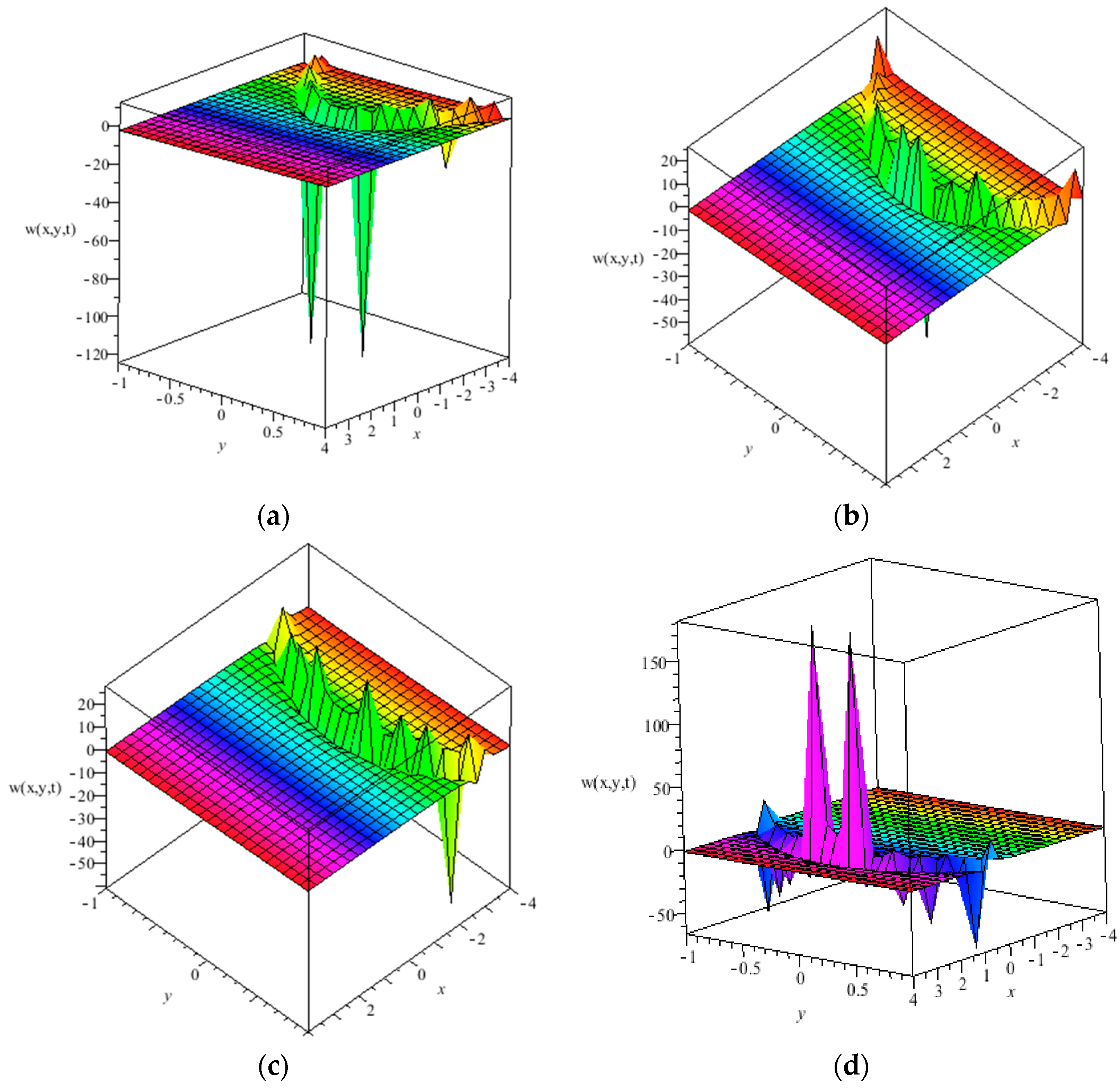
This result is plotted in Figure 2a–d as shown with different times and c values;
The result obtained in Equation (21) is different from the one obtained in [16] using hidden symmetries:
3.2. Similarity Reduction of Equation (2)
Lie vector reduces Equation (2) to
This equation possesses five Lie vectors:
Testing these vectors shows that the first two vectors are inherited from the original vectors as , while V3, V4, and V5 are hidden vectors.
3.2.1. Reduction of Equation (22)
We choose here to work only with the V4 Lie hidden vector, as it leads, in [1], to an ODE with no analytic solution:
where
As this equation has no analytic solution, we thus investigate the integrating factor method.
Integrating Factor Technique to Obtain Explicit Solutions
Equation (24) has two Integrating Factors:
They are used to reduce Equation (24) to a differential order:
This equation has two closed solutions:
where c and c1 are constants of integration. By back substitution for 𝜂 and θ(𝜂), we obtain
Differentiate w, r, t (x) once, we obtain
4. Analysis of Results
We then compare our results for vector V4; Equation (29) using the integrating Lie factor, with solutions obtained in [16] using two levels of hidden symmetries:
We find that these results obtained in [1], Equations (30) and (31), are different from our solution described in Equation (29).
5. Conclusions
In the present work, new solutions are found for the JM Equation (2);
- For vector X8 we replaced two successive Lie reduction processes used in [16] with a unique integrating process that led to new solutions.
- For vectors X2 + X5, we solved ODEs with no quadrature and obtained a new solution (Equation (29)) using an integrating factor, different from the solutions in [16] that resulted from a two consecutive Lie reductions.
- Thus, we can say that the advantages of using integrating factors are as follows:
- New and different solutions are obtained if we use a Lie symmetry reduction from A to z.
- The reduction stages are reduced via Lie symmetry reduction.
- In practice, the integrating factor method perhaps obtains the solution more easily than does the Lie reduction.
- The problems of the Lie symmetry reduction method (back substitution problems) are thus overcome.
Author Contributions
Rahma Sadat and Magda Kassem conceived the method; Rahma Sadat performed the calculations and Magda Kassem analyzed the results. Rahma Sadat wrote the paper, and Magda Kassem revised it.
Conflicts of Interest
The authors declare no conflict of interest.
References
- Bruzon, M.S.; Clarkson, P.A.; Gandarias, M.L.; Medina, E. The symmetry reductions of a turbulence model. J. Phys. A Math. Gen. 2001, 34, 3751–3760. [Google Scholar] [CrossRef]
- Xiao, H.; Young, Y.L.; Prevost, J.H. Parametric study of breaking solitary wave induced liquefaction of coastal sandy slopes. Ocean Eng. 2010, 37, 1546–1553. [Google Scholar] [CrossRef]
- Sarkar, S.; Basu, U.; De, S. (Eds.) Applied Mathematics; Springer: Kolkata, India, 2014. [Google Scholar]
- Biazar, J.; Eslami, M. A reliable algorithm for solving nonlinear Jaulent–Miodek equation. J. King Saud Univ. Sci. 2011, 23, 133–137. [Google Scholar] [CrossRef]
- Sadat, R.; Halim, A.A. New Soliton Solutions for the Kadomtsev-Petviashvili equation Using Darboux Transformation. Int. J. Mod. Math. Sci. 2017, 15, 112–122. [Google Scholar]
- El-Sayed, T.A.; El-Mongy, H.H. Application of variational iteration method to free vibration analysis of a tapered beam mounted on two-degree of freedom subsystems. Appl. Math. Model. 2018, in press. [Google Scholar] [CrossRef]
- Cariello, F.; Tabor, M. Painleve expansions for non integrable evolution equations. Phys. D 1989, 39, 77–94. [Google Scholar] [CrossRef]
- Wang, M.; Zhou, Y.; Li, Z. Applications of a homogenous balance method to exact solutions of nonlinear equation in mathematical physics. Phys. Lett. A 1996, 216, 67–75. [Google Scholar] [CrossRef]
- Fu, Z.T.; Liu, S.K.; Liu, S.D.; Zhao, Q. New Jacobi elliptic function expansion and new periodic solutions of nonlinear wave equations. Phys. Lett. A 2001, 290, 72–76. [Google Scholar] [CrossRef]
- Ma, W.-X.; Huang, T.; Zhang, Y. A multiple exp-function method for nonlinear differential equations and its application. Phys. Scr. 2010, 82, 065003. [Google Scholar] [CrossRef]
- He, J.-H.; Wu, X.-H. Exp-Function Method for Non-linear Wave Equations. Chaos Solitons Fractals 2006, 30, 700–708. [Google Scholar] [CrossRef]
- He, J.; Zhang, L. Generalized solitary solution and compacton-like solution of the Jaulent–Miodek equations using the Exp-function method. Phys. Lett. A 2008, 372, 1044–1047. [Google Scholar] [CrossRef]
- Sahoo, S.; Ray, S. New solitary wave solutions of time-fractional coupled Jaulent–Miodek equation by using two reliable methods. Nonlinear Dyn. 2016, 85, 1167–1176. [Google Scholar] [CrossRef]
- Wazwaz, A.-M. Multiple kink solutions and multiple singular kink solutions for (2 + 1)-dimensional nonlinear models generated by the Jaulent–Miodek hierarchy. Phys. Lett. A 2009, 373, 1844–1846. [Google Scholar] [CrossRef]
- Zhang, Y.; Liu, X.; Wang, G. Symmetry reductions and exact solutions of the (2 + 1)-dimensional Jaulent–Miodek equation. Appl. Math. Comput. 2012, 219, 911–916. [Google Scholar] [CrossRef]
- Rashed, A.S.; Kassem, M.M. Hidden symmetries and exact solutions of integro-differential Jaulent–Miodek evolution equation. Appl. Math. Comput. 2014, 247, 1141–1155. [Google Scholar] [CrossRef]
Figure 1.
(a) w(x, y, t) at c = 1, t = 0.3 s; (b) w(x, y, t) at c = 1, t = 0.5 s; (c) w(x, y, t) at c = 1, t = 0.8 s; (d) w(x, y, t) at c = 1, t = 1.2 s.
Figure 1.
(a) w(x, y, t) at c = 1, t = 0.3 s; (b) w(x, y, t) at c = 1, t = 0.5 s; (c) w(x, y, t) at c = 1, t = 0.8 s; (d) w(x, y, t) at c = 1, t = 1.2 s.

Figure 2.
(a) w(x, y, t) at c = 1, t = 0.3 s; (b) w(x, y, t) at c = 1, t = 0.5 s; (c) w(x, y, t) at c = 1, t = 0.8 s; (d) w(x, y, t) at c = −2, t = 0.8 s.
Figure 2.
(a) w(x, y, t) at c = 1, t = 0.3 s; (b) w(x, y, t) at c = 1, t = 0.5 s; (c) w(x, y, t) at c = 1, t = 0.8 s; (d) w(x, y, t) at c = −2, t = 0.8 s.

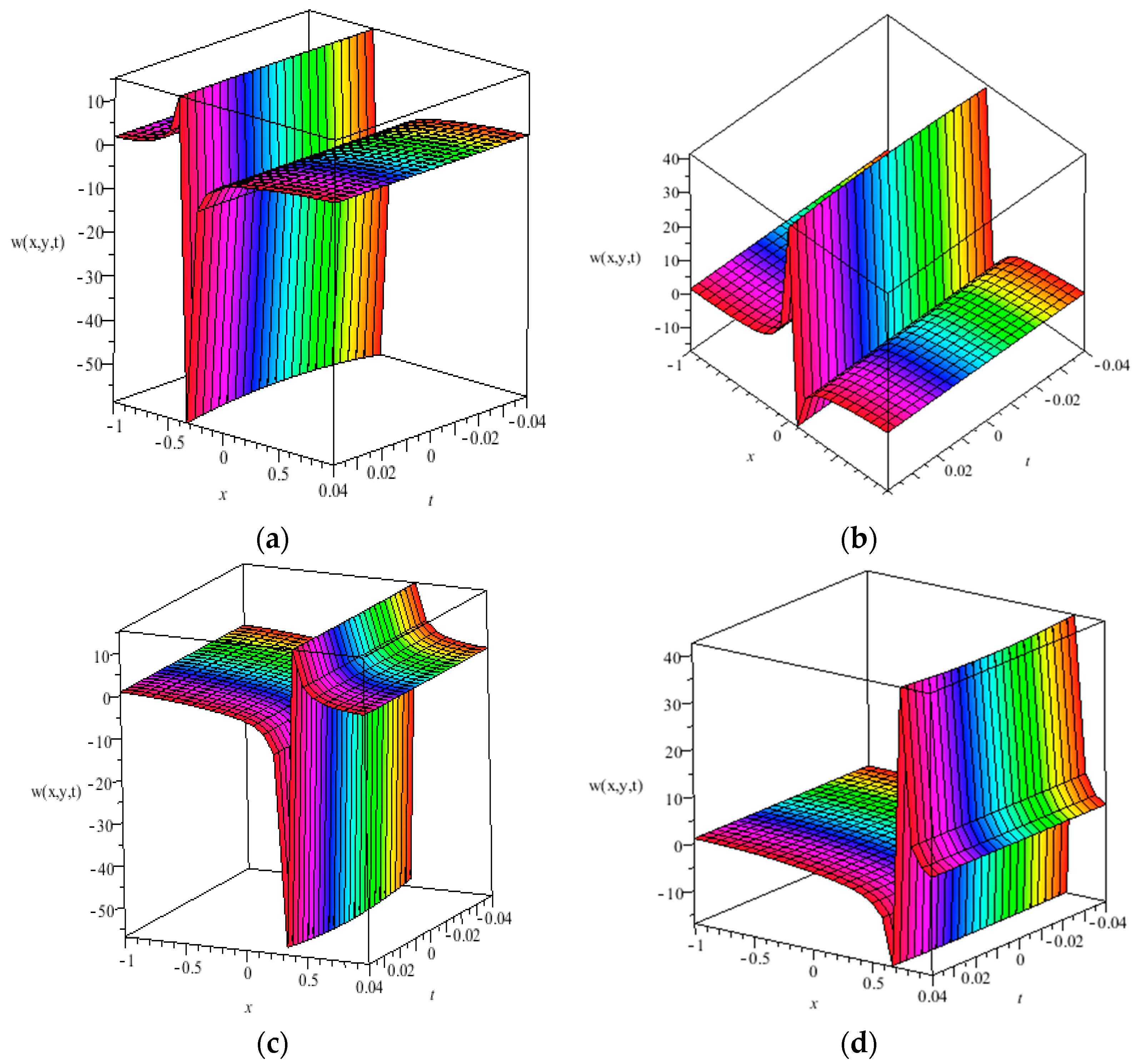
Figure 3.
(a) A positive solution of Equation (1.3) at c = 0; (b) a positive solution of Equation (1.3) at c = 1; (c) a negative solution of Equation (1.3) at c = 0; (d) a negative solution of Equation (1.3) at c = 1.
Figure 3.
(a) A positive solution of Equation (1.3) at c = 0; (b) a positive solution of Equation (1.3) at c = 1; (c) a negative solution of Equation (1.3) at c = 0; (d) a negative solution of Equation (1.3) at c = 1.
© 2018 by the authors. Licensee MDPI, Basel, Switzerland. This article is an open access article distributed under the terms and conditions of the Creative Commons Attribution (CC BY) license (http://creativecommons.org/licenses/by/4.0/).
Share and Cite
MDPI and ACS Style
Sadat, R.; Kassem, M. Explicit Solutions for the (2 + 1)-Dimensional Jaulent–Miodek Equation Using the Integrating Factors Method in an Unbounded Domain. Math. Comput. Appl. 2018, 23, 15. https://doi.org/10.3390/mca23010015
AMA Style
Sadat R, Kassem M. Explicit Solutions for the (2 + 1)-Dimensional Jaulent–Miodek Equation Using the Integrating Factors Method in an Unbounded Domain. Mathematical and Computational Applications. 2018; 23(1):15. https://doi.org/10.3390/mca23010015
Chicago/Turabian StyleSadat, Rahma, and Magda Kassem. 2018. "Explicit Solutions for the (2 + 1)-Dimensional Jaulent–Miodek Equation Using the Integrating Factors Method in an Unbounded Domain" Mathematical and Computational Applications 23, no. 1: 15. https://doi.org/10.3390/mca23010015