Article

Direct Solution of Second-Order Ordinary Differential Equation Using a Single-Step Hybrid Block Method of Order Five

Department of mathematics, College of Art and Sciences, Universiti Utara Sintok, Kedah 0060, Malaysia
*
Author to whom correspondence should be addressed.
These authors contributed equally to this work.
Math. Comput. Appl. 2016, 21(2), 12; https://doi.org/10.3390/mca21020012
Submission received: 1 February 2016 / Revised: 10 March 2016 / Accepted: 18 March 2016 / Published: 12 April 2016

Abstract

:
This paper proposes a new hybrid block method of order five for solving second-order ordinary differential equations directly. The method is developed using interpolation and collocation techniques. The use of the power series approximate solution as an interpolation polynomial and its second derivative as a collocation equation is considered in deriving the method. Properties of the method such as zero stability, order, consistency, convergence and region of absolute stability are investigated. The new method is then applied to solve the system of second-order ordinary differential equations and the accuracy is better when compared with the existing methods in terms of error.

1. Introduction

Ordinary differential equations (ODEs) are commonly used for mathematical modeling in many diverse fields such as engineering, operation research, industrial mathematics, behavioral sciences, artificial intelligence, management and sociology. This mathematical modeling is the art of translating problems from an application area into tractable mathematical formulations whose theoretical and numerical analysis provide insight, answers and guidance useful for the originating application [1]. This type of problem can be formulated either in terms of first-order or higher-order ODEs.
In this article, the system of second-order ODEs of the following form is considered.
y 1 = f 1 ( x , y 1 , y 1 ) ,    y 1 ( x 0 ) = a 0 , y 1 ( x 0 ) = b 0 y 2 = f 2 ( x , y 2 , y 2 ) , y 2 ( x 0 ) = a 1 , y 2 ( x 0 ) = b 1 y m = f m ( x , y m , y m ) ,     y m ( x 0 ) = a n , y m ( x 0 ) = b n
The method of solving higher-order ODEs by reducing them to a system of first-order approach involves more functions to evaluate them and then leads to a computational burden as mentioned in [2,3,4]. The multistep methods for solving higher-order ODEs directly have been developed by many scholars such as [5,6,7,8,9]. However, these researchers only applied their methods to solve single initial value problems of ODEs.
The aim of this paper is to develop a new numerical method for solving single second-order ODEs and systems of second-order ODEs directly.

2. Derivation of the Method

In this section, a one-step hybrid block method with three off-step points, x n + 1 5 ,   x n + 2 5 and x n + 3 5 , for solving Equation (1) is derived. Let the power series of the form
y j ( x ) = i = 0 v + m 1 a i ( x x n h ) i , j = 1 , , m .
be the approximate solution to Equation (1) for x [ x n , x n + 1 ] where n = 0 ,   1 ,   2 , , N 1 , a   s are the real coefficients to be determined, v is the number of collocation points, m is the number of interpolation points and h = x n x n 1 is a constant step size of the partition of interval [ a , b ] which is given by a = x 0 < x 1 < < x N 1 < x N = b .
Differentiating Equation (2) twice gives:
   y j ( x ) = f j ( x , y j , y j ) = i = 2 v + m 1 i ( i 1 ) a i h 2 ( x x n h ) i 2 , j = 1 , , m .
Interpolating Equation (2) at x n + 2 5 , x n + 3 5 and collocating Equation (3) at all points in the selected interval, i.e., x n , x n + 1 5 , x n + 2 5 , x n + 3 5 and x n + 1 , gives the following equations which can be written in matrix form:
( 1 2 5 4 25 8 125 16 625 32 3125 64 15625 1 3 5 9 25 27 125 81 625 243 3125 729 15625 0 0 2 h 2 0 0 0 0 0 0 2 h 2 6 5 h 2 12 25 h 2 4 25 h 2 6 125 h 2 0 0 2 h 2 12 5 h 2 48 25 h 2 32 25 h 2 96 125 h 2 0 0 2 h 2 18 5 h 2 108 25 h 2 108 25 h 2 486 125 h 2 0 0 2 h 2 6 h 2 12 h 2 20 h 2 30 h 2 ) ( a 0 a 1 a 2 a 3 a 4 a 5 a 6 ) = ( y j n + 2 5 y j n + 3 5 f j n f j n + 1 5 f j n + 2 5 f j n + 3 5 f j n + 1 ) , j = 1 , , m .
Employing the Gaussian elimination method on Equation (4) gives the coefficient ai 's, for i = 0 ( 1 ) 6 . These values are then substituted into Equation (2) to give the implicit continuous hybrid method of the form:
y j ( x ) = i = 2 5 , 3 5 α j i ( x )    y j n + i + i = 1 5 , 2 5 , 3 5 β j i ( x )    f j n + i + i = 0 1 β j i ( x )    f j n + i , j = 1 , , m ..
Differentiating Equation (5) once yields:
y j ( x ) = i = 2 5 , 3 5 d d x α j i ( x )    y j n + i + i = 1 5 , 2 5 , 3 5 d d x β j i ( x )    f j n + i + i = 0 1 d d x β j i ( x )    f j n + i , j = 1 , , m .
where
α j n + 3 5 = ( 5 ( x x n ) h 2 )
α j n + 2 5 = ( 3 5 ( x x n ) h )
β j 0 = ( x x n ) 2 2 61 ( x x n ) 3 36 h + 205 ( x x n ) 4 72 h 2 55 ( x x n ) 5 24 h 3 + 25 ( x x n ) 6 36 h 4 301 h ( x x n ) 4500 + 11 h 2 3750
β j 1 5 = 25 ( x x n ) 3 8 h 775 ( x x n ) 4 96 h 2 + 125 ( x x n ) 5 16 h 3 125 ( x x n ) 6 48 h 4 25 h ( x x n ) 96 + 83 h 2 2000
β j 2 5 = 575 ( x x n ) 4 72 h 2 25 ( x x n ) 3 12 h 75 ( x x n ) 5 8 h 3 + 125 ( x x n ) 6 36 h 4 43 h ( x x n ) 300 + 17 h 2 250
β j 3 5 = 25 ( x x n ) 3 36 h 425 ( x x n ) 4 144 h 2 + 25 ( x x n ) 5 6 h 3 125 ( x x n ) 6 72 h 4 109 h ( x x n ) 3600 + 23 h 2 3000
β j 1 = 55 ( x x n ) 4 288 h 2 ( x x n ) 3 24 h 5 ( x x n ) 5 16 h 3 + 25 ( x x n ) 6 144 h 4 + 11 h ( x x n ) 12000 h 2 10000
Equation (5) is evaluated at non-interpolating points, i.e., xn, x n + 1 5 and xn+1, while its first derivative is evaluated at all points, and this yields the following equation in matrix form:
A j    Y j L = B j    R j 1 + C j    R j 2 + D j    R j 3   j = 1 , , m
where
A j = ( 0 3 2 0 0 0 0 0 1 2 1 0 0 0 0 0 0 2 3 1 0 0 0 0 0 5 h 5 h 0 0 0 0 0 0 5 h 5 h 0 1 0 0 0 0 5 h 5 h 0 0 1 0 0 0 5 h 5 h 0 0 0 1 0 0 5 h 5 h 0 0 0 0 1 ) ,   Y j L = ( y n + 1 5 y n + 2 5 y n + 3 5 y n + 1 y n + 1 5 y n + 2 5 y n + 3 5 y n + 1 ) ,   B j = ( 1 0 0 0 0 0 0 1 0 0 0 0 0 0 0 0 ) ,   R 1 = ( y n y n )
C = ( 11 h 2 3750 h 2 7500 21 h 2 2500 301 h 4500 7 h 1800 h 500 19 h 9000 53 h 1000 ) ,   R j 2 = ( f j n )   D j = ( 83 h 2 2000 17 h 2 250 23 h 2 3000 h 2 10000 23 h 2 6000 49 h 2 1500 11 h 2 3000 h 2 30000 83 h 2 2000 113 h 2 1500 151 h 2 1000 337 h 2 30000 25 h 96 43 h 300 109 h 3600 11 h 12000 69 h 800 371 h 1800 41 h 3600 h 7200 31 h 2400 77 h 900 31 1200 17 h 36000 31 h 2400 31 h 600 43 h 720 7 h 12000 25 h 96 883 h 1800 797 h 1200 4283 h 36000 ) ,   R j 3 = ( f j n + 1 5 f j n + 2 5 f j n + 3 5 f j n + 1 )
Multiplying Equation (7) by A j 1 gives the hybrid block method as shown below.
I    Y j L = B ¯ j    R j 1 + C ¯ j    R j 2 + D ¯ j    R j 3
I = ( 1 0 0 0 0 0 0 0 0 1 0 0 0 0 0 0 0 0 1 0 0 0 0 0 0 0 0 1 0 0 0 0 0 0 0 0 1 0 0 0 0 0 0 0 0 1 0 0 0 0 0 0 0 0 1 0 0 0 0 0 0 0 0 1 ) ,   B ¯ j = ( 1 h 5 1 2 h 5 1 3 h 5 1 h 0 1 0 1 0 1 0 1 ) ,   C ¯ j = ( 58 h 2 5625 134 h 2 2500 93 h 2 2500 h 2 18 637 h 9000 73 h 1125 69 h 1000 h 72 ) ,   D ¯ j = ( 173 h 2 12000 h 2 150 37 h 2 18000 7 h 2 60000 47 h 2 750 4 h 2 375 h 2 225 h 2 3750 459 h 2 4000 9 h 2 500 21 h 2 2000 9 h 2 20000 25 h 96 2 0 25 h 2 144 h 2 96 209 h 1200 113 h 1800 17 h 900 19 h 18000 41 h 150 13 h 225 h 225 h 2250 99 h 400 39 h 200 9 h 100 3 h 2000 25 h 48 25 h 72 25 h 36 17 h 144 )

3. Properties of the Method

3.1. Zero Stability

The one-step hybrid block method (8) is said to be zero-stable if and only if the first characteristic function Π(x) has roots such that | x t | 1 and if | x t | = 1 ; then the multiplicity of x t does not exceed two. The characteristic function of the new derived method is given as below:
Π ( x ) = ( 1 0 0 0 0 0 0 0 0 1 0 0 0 0 0 0 0 0 1 0 0 0 0 0 0 0 0 1 0 0 0 0 0 0 0 0 1 0 0 0 0 0 0 0 0 1 0 0 0 0 0 0 0 0 1 0 0 0 0 0 0 0 0 1 ) ( 0 0 0 1 0 0 0 h 5 0 0 0 1 0 0 0 2 h 5 0 0 0 1 0 0 0 3 h 5 0 0 0 1 0 0 0 1 0 0 0 0 0 0 0 1 0 0 0 0 0 0 0 1 0 0 0 0 0 0 0 1 0 0 0 0 0 0 0 1 ) = x 6 ( x 1 ) 2
the solution of which is x = 0 , 0 , 0 , 0 , 0 , 0 , 1 , 1 . Hence, our method is zero-stable.

3.2. Order of the Method

According to [9] the order of the new method in Equation (8) is obtained by using the Taylor series and it is found that the developed method has an order of [ 5 , 5 , 5 , 5 , 5 , 5 , 5 , 5 ] T with an error constant vector of:
[1.732063 × 10⁻⁷, 4.104127 × 10⁻⁷, 6.582857 × 10⁻⁷, −1.587302 × 10⁻⁶, 1.537778 × 10⁻⁶, 8.533333 × 10⁻⁷,
1.680000 × 10⁻⁶, −1.666667 × 10⁻⁵]T

3.3. Consistency

The hybrid block method is said to be consistent if it has an order more than or equal to one. Therefore, our method is consistent.

3.4. Convergence

Zero stability and consistency are sufficient conditions for a linear multistep method to be convergent [10]. Since the new hybrid block method is zero-stable and consistent, it can be concluded that the method is convergent.

3.5. Region of Absolute Stability

In this section, the locus boundary method is adopted to determine the region of absolute stability. The linear multistep numerical method is said to be absolutely stable if for all given h, the roots of the characteristic function Π ( x ) = ρ ( x ) h ¯ σ ( x ) satisfies | x | < 1 . The test equation y = λ 2 y is substituted in Equation (8) where h ¯ = λ 2 h 2 and λ = d f d y . Substituting x = cos θ i sin θ and equating the imaginary part yields:
h ¯ = ( 56250000 ( cos ( θ ) - 1 ) ) ( 3 cos ( θ ) - 89 )
This gives the stability interval of (0, 1222826).

4. Implementation of the Method

The initial starting value at each block is obtained by using the Taylor method. Then, the calculations are corrected using Equation (8). For the next block, the same techniques are repeated to compute the approximation values of y j n + 1 5 , y j n + 2 5 , y j n + 3 5 , y j n + 1 , j = 1,…, m simultaneously until the end of the integrated interval. During the calculations of the iteration, the final values of y j n + 1 are taken as the initial values for the next iteration.

5. Numerical Experiments

In this section, the performance of the developed one-step hybrid block method is examined using the following three systems of second-order initial value problems. Table 1 and Table 2, Table 3 and Table 4, and Table 5 and Table 6 show the comparison of the numerical results of the new method with exact solution for solving problems 1–3 respectively. While, in 
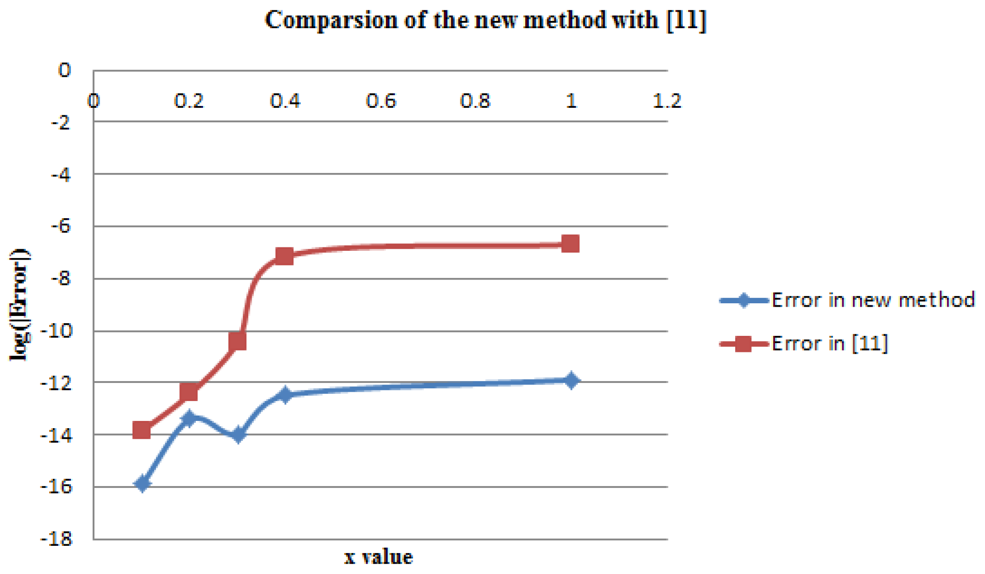
Table 7, the results of the developed method are more accurate than that of [11] which was executed by six-step block method for solving Problem 4.
Problem 1: 
y 1 = 1 cos x + s i n ( y 2 ) + cos ( y 2 )   y 1 ( 0 ) = 1 ,   y 1 ( 0 ) = 0 ,
y 2 = 1 ( 4 + y 1 2 ) 1 ( 5 sin ( x ) 2 )   y 2 ( 0 ) = 0 ,   y 2 ( 0 ) = π ,
Exact solution: y1 = cos x, y2 = πx
Problem 2: 
y 1 = e x y 2   y 1 ( 0 ) = 1 ,   y 1 ( 0 ) = 0 ,   h = 0.01
y 2 = 2 e x y 1   y 2 ( 0 ) = 1 ,   y 2 ( 0 ) = 1 ,
Exact solution: y1 = cos x, y2 = ex cos x
Problem 3: 
y 1 = y 1 y 1 2 + y 2 2   y 1 ( 0 ) = 1 ,   y 1 ( 0 ) = 0 , h = 0.01
y 2 = y 2 y 1 2 + y 2 2   y 2 ( 0 ) = 0 ,   y 2 ( 0 ) = 1 ,
Exact solution: y1 = cos x, y2 = sin x
Problem 4: 
y = x ( y ) 2   ,   y ( 0 ) = 1 ,   y ( 0 ) = 1 2 ,   h = 1 30 .
Exact solution y = 1 + 1 2 l n ( 2 + x 2 _ x )  
The numerical results confirm that the proposed method produces better accuracy if compared with the existing methods. This is also clear in the graph below (Figure 1).

6. Conclusions

In this article, a one-step block method with three off-step points is derived via the interpolation collocation approach. The developed method is consistent, zero-stable, convergent, with a region of absolute stability and order five. The numerical results generated when the new developed method was applied to three systems of second-order initial value problems above have shown the high accuracy of the new method.

Author Contributions

Both authors equally contributed to this work.

Conflicts of Interest

The authors declare no conflict of interest.

References

  1. Omar, Z.; Sulaiman, M. Parallel r-point implicit block method for solving higher order ordinary differential equations directly. J. ICT 2004, 3, 53–66. [Google Scholar]
  2. Kayode, S.J.; Adeyeye, O. A 3-step hybrid method for direct solution of second order initial value problems. Aust. J. Basic Appl. Sci. 2011, 5, 2121–2126. [Google Scholar]
  3. James, A.; Adesanya, A.; Joshua, S. Continuous block method for the solution of second order initial value problems of ordinary differential equation. Int. J. Pure Appl. Math. 2013, 83, 405–416. [Google Scholar] [CrossRef]
  4. Omar, Z.; Suleiman, M.B. Parallel two-point explicit block method for solving high-order ordinary differential equations. Int. J. Simul. Process Model. 2006, 2, 227–231. [Google Scholar] [CrossRef]
  5. Vigo-Aguiar, J.; Ramos, H. Variable stepsize implementation of multistep methods for y = f (x, y, y’). J. Comput. Appl. Math. 2006, 192, 114–131. [Google Scholar] [CrossRef]
  6. Adesanya, A.O.; Anake, T.A.; Udo, O. Improved continuous method for direct solution of general second order ordinary differential equations. J. Niger. Assoc. Math. Phys. 2008, 13, 59–62. [Google Scholar]
  7. Awoyemi, D.O. A P-stable linear multistep method for solving general third order of ordinary differential equations. Int. J. Comput. Math. 2003, 80, 985–991. [Google Scholar] [CrossRef]
  8. Henrici, P. Some Applications of the Quotient-Difference Algorithm. Proc. Symp. Appl. Math. 1963a, 15, 159–183. [Google Scholar]
  9. Lambert, J.D. Computational Methods in ODEs; John Wiley and Sons: New York, NY, USA, 1973. [Google Scholar]
  10. Henrici, P. Discrete Variable Methods in ODE; John Wiley and Sons: New York, NY, USA, 1962. [Google Scholar]
  11. Kuboye, J.O.; Omar, Z. Derivation of a Six-Step Block method for direct solution of second order ordinary differential Equations. Math. Comput. Appl. 2015, 20, 151–159. [Google Scholar] [CrossRef]
Figure 1. Comparison between errors in the new method with error in [11] for solving Problem 4.
Mca 21 00012 g001
Table 1. Exact solution and computed solution of the new method for solving y1 in Problem 1.
xExact Solution of y1Computed Solution of y1Error in y1
0.2 0.98006657784124163 0.98006661117494787 3.333371 × 10⁻⁸
0.4 0.92106099400288510 0.92106172165508671 7.276522 × 10⁻⁷
0.6 0.82533561490967833 0.82533871008804471 3.095178 × 10⁻⁶
0.8 0.69670670934716550 0.69671472046421035 8.011117 × 10⁻⁶
1.0 0.54030230586813977 0.54031839116566260 1.608530 × 10⁻⁵
Table 2. Exact solution and computed solution of the new method for solving y2 in Problem 1.
xExact solution of y2Computed solution of y2Error in y2
0.20.628318530717958620.628318530712221555.737077 × 10−12
0.41.256637061435917201.256637061096243403.396738 × 10−10
0.61.884955592153875901.884955588674244403.479631 × 10−9
0.82.513274122871834502.513274106263250701.660858 × 10−8
1.03.141592653589792703.141592601227237505.236256 × 10−8
Table 3. Exact solution and computed solution of the new method for solving y1 in Problem 2.
xExact Solution of y1Computed Solution of y1Error in y1
0.20.9800665778412416300.9800665744927760103.348466 × 10−9
0.40.9210609940028849900.9210609612374383003.276545 × 10−8
0.60.8253356149096781100.8253354816882978501.332214 × 10−7
0.8 0.69670670934716505 0.6967063547191876303.546280 × 10−7
1.00.5403023058681392100.5403015703504631107.355177 × 10−7
Table 4. Exact solution and computed solution of the new method for solving y2 in Problem 2.
xExact Solution of y2Computed Solution of y2Error in y2
0.21.1970560213558914001.1970566517697601006.304139 × 10−7
0.41.3740615388875221001.3740640605564765002.521669 × 10−6
0.61.5038595405587862001.5038649701514313005.429593 × 10−6
0.81.5505492968074224001.5505581495881100008.852781 × 10−8
1.01.4686939399158849001.4687058868689173001.194695 × 10−8
Table 5. Exact solution and computed solution of the new method for solving y1 in Problem 3.
xExact Solution of y1Computed Solution of y1Error in y1
0.20.9800665778412416300.9800665777991555104.208611e−11
0.4 0.921060994002884990 0.9210609937083160702.945689e−10
0.60.8253356149096781100.8253356141500253207.596528e−10
0.80.6967067093471650500.6967067081685610601.178604e−9
1.00.5403023058681392100.5403023046878443501.180295e−9
Table 6. Exact solution and computed solution of the new method for solving y2 in Problem 3.
xExact Solution of y2Computed Solution of y2Error in y2
0.20.1986693307950612400.1986693311137544003.186932 × 10−10
0.40.3894183423086506900.3894183433914287801.082778 × 10−9
0.60.5646424733950355900.5646424751681853301.773150 × 10−9
0.80.7173560908995231200.7173560927622033601.862680 × 10−9
1.00.8414709848078968400.8414709858895288401.081632 × 10−9
Table 7. Comparison of the new method with [11] for solving Problem 4.
xExact SolutionComputed SolutionError in New Method P = 5Error in [11] P = 7
0.11.05004172927849141.05004172927850451.310063 × 10−161.445510 × 10⁻¹⁴
0.21.10033534773107561.10033534773111533.974598 × 10−143.779332 × 10⁻¹³
0.31.15114043593646681.15114043593645651.021405 × 10−143.428134 × 10⁻¹¹
0.41.20273255405408211.20273255405375173.304024 × 10−136.987109 × 10⁻⁸
1.01.25541281188299521.25541281188170251.292744 × 10−122.017066 × 10⁻⁷

