General Solution of the Extended Plate Model Including Diffusion, Slow Transfer Kinetics and Extra-Column Effects for Isocratic Chromatographic Elution

Abstract

The plate model proposed by Martin and Synge has been used for the characterization of columns up-to-date. In this approach, the column is divided into a large number (N) of identical theoretical plates. Mobile phase transference between plates takes place in infinitesimal steps with mixing of the solutions in the adjacent plates during the flow. The plate height is related to the band broadening that occurs in the mixing process due to the microscopic heterogeneities in the mobile phase flow. According to the original Martin and Synge model, solutes reach the equilibrium instantaneously in each theoretical plate, where dispersion is produced by: (i) convection or mixing of the mobile phase reaching a theoretical plate with that existing in that plate; and (ii) the equilibrium of the solute that is partitioned between mobile phase and stationary phase. In this work, a general method is proposed to solve the problem of chromatographic elution by means of an extended plate model assuming slow mass transfer, longitudinal diffusion in both mobile phase and stationary phase, and the extra column dispersion. The final equation was validated by comparing the results with those obtained through the numerical simulation of the solute migration using the finite differential approach. Experimental data were also used to check the validity of the derived equations.

1. Introduction

In 1941, Martin and Synge developed the principles of partition chromatography [1,2], and proposed the theoretical plate model to describe the elution in linear chromatography. These authors introduced the concept of “theoretical plate” in analogy to the description of fractional distillation [3]. In 1952, both researchers were awarded with the Nobel Prize [4]. Because of its simplicity, the plate model was useful to measure the chromatographic column performance through the proposal of the concept of number of column theoretical plates (N). Later, Craig [5] introduced the counter-current distribution and derived a mathematical treatment to explain the experimental results [6]. In the plate model, the theoretical plate is represented as a column disk of very small thickness, where the equilibrium is reached instantaneously. In the Craig model, the elution is discontinuous and at each step the mobile phase inside a theoretical plate is replaced completely by the mobile phase in the preceding plate. In that time interval, the distribution equilibrium is assumed to be reached. This process results in a peak showing a binomial distribution [7], which can be approximated to a Gaussian with a variance equal to:

$${\mathsf{\sigma }}^2=\frac{t_{\mathrm{R}}(t_{\mathrm{R}}-t_0)}{N}$$

(1)

where t_R and t₀ are the retention time and dead time, respectively. According to this model, a non-retained compound would give rise to a peak with null width; hence, the peak broadening modeled by Equation (1) is due solely to the equilibrium between mobile phase and stationary phase.

Instead, according to Martin and Synge, the elution is continuous and the mobile phase is transferred from one plate to the next in infinitesimal volumes, and the incoming phase is mixed with the theoretical plate receiver. Therefore, the proposed model implies an additional broadening due to this convective effect. Martin and Synge originally solved the plate model by the sequential study of the infinitesimal steps taking place during the elution process. Later, Said [8,9] performed a treatment based on the continuous flow of eluent through the column plates. More recently, we have studied the elution process by solving a system of differential equations consisting of mass balances that occur in each plate [10]. For plate i:

$$\frac{\mathrm{d}{n}_i}{dt}=\frac{N}{t_0(1+k)}{n}_{i-1}-\frac{N}{t_0(1+k)}{n}_i$$

(2)

where k is the retention factor and n_i the moles of solute in plate i at time t. The analytical solution of the system of differential equations yields the following peak profile versus time [7,10]:

$$f(t)={\left(\frac{N}{t_0(1+k)}\right)}^N\frac{t^{N-1}}{(N-1)!}{e}^{\frac{-N}{t_0(1+k)}t}$$

(3)

Equation (3) describes an Erlang distribution [11], which for sufficiently large values of N, tends to a normal distribution [7], with mean and variance equal to:

$$t_{\mathrm{R}}=t_0(1+k)$$

(4)

$${\mathsf{\sigma }}^2=\frac{t_{\mathrm{R}}^2}{N}$$

(5)

In the Martin and Synge model, when a solute does not interact with the stationary phase, peak broadening is given by:

$${\mathsf{\sigma }}_0^2=\frac{t_0^2}{N}$$

(6)

The plate model theory described by Martin and Synge has been adopted as a basis for defining the efficiency and separation capability of chromatographic columns up-to-date. Despite its popularity, the plate model had only been solved for the simplest case that considers only the instantaneous equilibrium. By applying the Laplace transform, we managed to consider a slow mass transfer between mobile phase and stationary phase [10], proposing the following dispersion equation:

$${\mathsf{\sigma }}^2=\frac{t_{\mathrm{R}}^2}{N}\left(1+2\left(\frac{\mathsf{\tau }}{\mathsf{\nu }}\right)\frac{k}{1+k}\right)$$

(7)

where τ is a parameter related with the mass transfer due to the flow, and ν is the mass transfer constant between phases.

A more comprehensive study of the chromatographic elution process requires considering besides the equilibrium and slow mass transfer kinetics between mobile phase and stationary phase, the longitudinal diffusion in the mobile phase (and to a lesser extent, in the stationary phase), together with the eddy diffusion and heterogeneities in the flow [12,13]. In addition, the dispersion due to extra-column sources should be included [14,15]. The rate models [16] have been most widely used to consider some of these factors in both linear and non-linear elution [17], and for isocratic and gradient elution [18]. However, its resolution can be difficult and requires several approximations [17,19], or the use of numerical methods [20,21,22]. When an equilibrium with slow mass transfer and diffusion in the mobile phase is considered, the differential mass balance in an infinitesimal column segment can be expressed as:

$$\frac{\partial c}{\partial t}+u\frac{\partial c}{\partial x}+\mathsf{\Phi }\frac{\partial q}{\partial t}=D_{\mathrm{m}}\frac{{\partial }^{2}c}{\partial x^2}$$

(8)

In the solid-film linear driving-force model, the rate of concentration change in the stationary phase is given by:

$$\frac{\partial q}{\partial t}=k_{\mathrm{f}}(q^{*}-q)=k_{\mathrm{f}}(Kc-q)$$

(9)

and the differential equations can be solved as [18,23]:

$${\mathsf{\sigma }}^2=\frac{t_{\mathrm{R}}^2}{L}\left(\frac{2D_{\mathrm{m}}}{u}+2\frac{k}{{(1+k)}^2}\frac{u}{k_{\mathrm{f}}}\right)$$

(10)

In Equations (8)–(10), c and q are the concentration of the solute in the mobile phase and stationary phase, respectively; x is the axial coordinate along the column; u is the linear flow velocity; q* is the theoretical concentration of solute at equilibrium with c in the mobile phase; Φ is the volume phase ratio (Φ = V_s/V_m, where V_s and V_m are the volumes of stationary phase and mobile phase, respectively); D_m is the solute diffusion coefficient in the mobile phase; k_f is the mass transfer rate between phases; K is the partition constant; and L is the column length.

Band broadening is usually expressed in terms of column plate height (H):

$$H=\frac{L{\mathsf{\sigma }}^2}{t_{\mathrm{R}}^2}$$

(11)

Accordingly, Equation (10) is developed as:

$$H=2\mathsf{\lambda }{d}_{\mathrm{p}}+2\frac{D_{\mathrm{m}}}{u}+2\frac{k}{{(1+k)}^2}\frac{u}{k_{\mathrm{f}}}=A+\frac{B}{u}+Cu$$

(12)

where the first term has been added to take into account the eddy diffusion. A, B and C are constants that account for the contributions to band broadening from the eddy diffusion, longitudinal diffusion, and mass transfer resistance, respectively. This equation is known as “van Deemter equation” [24], and provides a basis to study the properties of chromatographic columns (column performance) that affect the peak shape, usually characterized by relating H to the linear mobile phase velocity (u), showing the different contributions to band broadening [25].

In another approach, proposed by Giddings and Eyring [26], the random migration of a single molecule is considered from a probabilistic point of view to describe the distribution function of the solute in the elution process [27], the elution profile being the probability density function of the retention time of the individual molecules. Recently, Chen [28] obtained identical results with this approach to those provided by the macroscopic models.

Other studies have described the band dispersion as a combination of independent processes, being the global variance the summation of the individual variances [29,30,31]:

$${\mathsf{\sigma }}^2={\mathsf{\sigma }}_{\mathrm{E}}^2+{\mathsf{\sigma }}_{\mathrm{d}}^2+{\mathsf{\sigma }}_{\mathrm{s}}^2+{\mathsf{\sigma }}_{\mathrm{ext}}^2$$

(13)

where ${\mathsf{\sigma }}_{\mathrm{E}}^2$, ${\mathsf{\sigma }}_{\mathrm{d}}^2$, ${\mathsf{\sigma }}_{\mathrm{s}}^2$ and ${\mathsf{\sigma }}_{\mathrm{ext}}^2$ are the variance associated to the eddy diffusion, longitudinal diffusion, slow mass transfer, and external factors, respectively. Therefore, each mechanism can be studied separately. Thus, for example, Knox et al. included the molecular diffusion in the stationary phase by considering it as a random walk process, where the theoretical plate height was given by [32]:

$$H_{\mathrm{d}}=2\frac{{\mathsf{\gamma }}_{\mathrm{m}}{D}_{\mathrm{m}}+k{\mathsf{\gamma }}_{\mathrm{s}}{D}_{\mathrm{s}}}{u}$$

(14)

where the subscripts m and s account for the mobile phase and stationary phase, respectively, γ is the obstruction factor, D the diffusion coefficient, and the products γD quantify the effective diffusion coefficients.

Following these approaches, several equations similar to Equation (12) have been developed [19,33,34] to explain the behavior of the theoretical plate height at varying mobile phase velocity. According to Knox, the most important contribution to dispersion under practical operating conditions comes from factors affecting the term A in Equation (12), the slow mass transfer within the porous particles being usually unimportant [35,36]. On the other hand, Desmet et al. has reviewed the expression for term B [37], using a numerical procedure. A significant deviation was shown from the Knox type expression traditionally employed in high-performance liquid chromatography (HPLC).

In this work, a general approach is proposed to describe the peak broadening in liquid chromatography by applying an extended plate model that assumes slow mass transfer, the longitudinal diffusion in both mobile phase and stationary phase, and the extra-column contributions. The results have been validated by comparison with those obtained by simulating the elution using a finite difference approach. Experimental data were also used to check the validity of the derived equations.

2. Theory

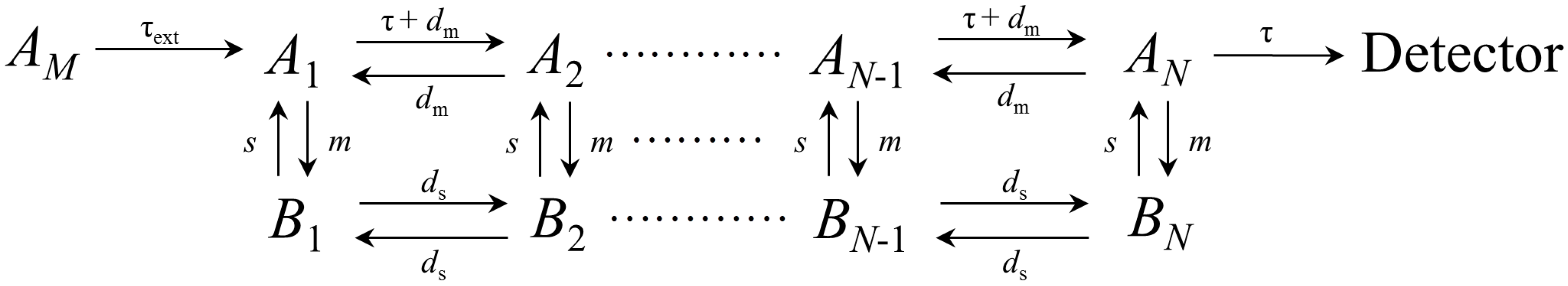
2.1. General Description of the Chromatographic Elution Based on the Extended Plate Model

The next conditions will be considered to develop the approach:

(i)

The solute crosses a fixed length L inside the column.

(ii)

The column is divided into N equal microscopic theoretical plates.

(iii)

The interaction between solute and stationary phase in each theoretical plate is determined by a linear isotherm:

$$K=\frac{{[B]}_i^{*}}{{[A]}_i^{*}}=\frac{b_i^{*}}{a_i^{*}}\frac{V_{\mathrm{m}}}{V_{\mathrm{s}}}=k\frac{V_{\mathrm{m}}}{V_{\mathrm{s}}}$$

(15)

where ${[A]}_i^{*}$ and ${[B]}_i^{*}$ are the solute concentration in the mobile phase and stationary phase, respectively, at equilibrium inside the i theoretical plate, and $b_i^{*}$ and $a_i^{*}$ the corresponding number of moles.

In the theoretical plate theory, the column is divided into N microscopic and equal segments through which the mobile phase moves. The solute mass transfer between adjacent theoretical plates is influenced by the mobile phase flow, the mass transfer between mobile phase and stationary phase, and the longitudinal diffusion in both mobile phase and stationary phase. The mass balance between adjacent plates can be described by the differential equations given below. The transfer component due to the mobile phase flow is first quantified through [10]:

$${\left(\frac{\partial a_i}{\partial t}\right)}_{\mathrm{flow}}=\mathsf{\tau }{a}_{i-1}-\mathsf{\tau }{a}_i$$

(16)

where a_i is the number of moles in the mobile phase inside the theoretical plate i, and τ the flow rate expressed as the number of theoretical plates per time unit:

$$\mathsf{\tau }=\frac{N}{t_0}=\frac{u}{H}=\frac{F}{V_{\mathrm{m}}}$$

(17)

where F is the mobile phase flow rate.

The mass transfer between mobile phase and stationary phase in each theoretical plate is described by the following equation [13]:

$${\left(\frac{\partial a_i}{\partial t}\right)}_{\mathrm{transfer}}=\mathsf{\nu }(a_i^{*}-a_i)$$

(18)

where ν is the mass-transfer rate constant and $a_i^{*}$ the moles of solute in the mobile phase when the equilibrium is reached. Considering that:

$$a_i^{*}+b_i^{*}=a_i+b_i$$

(19)

and assuming a linear isotherm as in Equation (15), the next expression is derived:

$${\left(\frac{\partial a_i}{\partial t}\right)}_{\mathrm{transfer}}=\frac{\mathsf{\nu }}{1+k}{b}_i-\frac{\mathsf{\nu }k}{1+k}{a}_i=s{b}_i-m{a}_i$$

(20)

where s and m are the kinetic constants for the slow mass transfer of the solute from the stationary phase and mobile phase, respectively.

Similarly, the change in the number of moles of solute in the stationary phase will be given by:

$${\left(\frac{\partial b_i}{\partial t}\right)}_{\mathrm{transfer}}=m{a}_i-s{b}_i$$

(21)

Finally, the flow expressed as moles per unit area and time between two theoretical plates, due to the longitudinal diffusion, will be given by the Fick’s law [7]. For the mobile phase:

$$J=-D_{\mathrm{m}}\frac{\mathrm{d}c}{\mathrm{d}x}\cong -D_{\mathrm{m}}\frac{\mathrm{\Delta }c}{H}$$

(22)

where D_m is the diffusion coefficient (length²·time^‒1), Δc the difference in the solute concentration between two adjacent plates, and H the theoretical plate height; that is, the distance between the center of both plates. The change in the number of moles of solute in the mobile phase between two adjacent plates will be:

$$SJ=-S{D}_{\mathrm{m}}\frac{\mathrm{\Delta }a}{H{V}_{\mathrm{m}}}=-\frac{D_{\mathrm{m}}}{H^2}\mathrm{\Delta }a=-d_{\mathrm{m}}\mathrm{\Delta }a$$

(23)

where S is the mobile phase area, V_m = SH, and Δa is the difference in the number of moles between two adjacent plates. Therefore, taking into account the two theoretical plates adjacent to plate i, it results:

$${\left(\frac{\partial a_i}{\partial t}\right)}_{\mathrm{diffusion}}=d_{\mathrm{m}}\left(a_{i+1}-a_i\right)-d_{\mathrm{m}}\left(a_i-a_{i-1}\right)$$

(24)

for the mobile phase and

$${\left(\frac{\partial b_i}{\partial t}\right)}_{\mathrm{diffusion}}=d_{\mathrm{s}}\left(b_{i+1}-b_i\right)-d_{\mathrm{s}}\left(b_i-b_{i-1}\right)$$

(25)

for the stationary phase, where d_m and d_s are the diffusion transfer kinetic constants for the mobile phase and stationary phase, respectively:

$$d_{\mathrm{m}}=\frac{D_{\mathrm{m}}}{H^2}$$

(26a)

$$d_{\mathrm{s}}=\frac{D_{\mathrm{s}}}{H^2}$$

(26b)

The change in the number of moles of solute due to all the described processes for plate i will be:

$$\frac{\mathrm{d}{a}_i}{\mathrm{d}t}=-\mathsf{\tau }(a_i-a_{i-1})-m{a}_i+s{b}_i+d_{\mathrm{m}}(a_{i+1}-a_i)-d_{\mathrm{m}}(a_i-a_{i-1})$$

(27)

$$\frac{\mathrm{d}{b}_i}{\mathrm{d}t}=m{a}_i-s{b}_i+d_{\mathrm{s}}(b_{i+1}-b_i)-d_{\mathrm{s}}(b_i-b_{i-1})$$

(28)

For the whole column, the following system of differential equations can be outlined:

$$\begin{array}{l}{a}_1^{(1)}={\mathsf{\tau }}_{\mathrm{ext}}{a}_{M,\mathrm{ext}}-\mathsf{\tau }{a}_1-m{a}_1+s{b}_1+d_{\mathrm{m}}(a_2-a_1)\\ b_1^{(1)}=m{a}_1-s{b}_1+d_s(b_2-b_1)\\ ⋮\\ a_i^{(1)}=-\mathsf{\tau }(a_i-a_{i-1})-m{a}_i+s{b}_i+d_{\mathrm{m}}(a_{i+1}-a_i)-d_{\mathrm{m}}(a_i-a_{i-1})\\ b_i^{(1)}=m{a}_i-s{b}_i+d_{\mathrm{s}}(b_{i+1}-b_i)-d_{\mathrm{s}}(b_i-b_{i-1})\\ ⋮\\ a_N^{(1)}=-\mathsf{\tau }(a_N-a_{N-1})-m{a}_N+s{b}_N-d_{\mathrm{m}}(a_N-a_{N-1})\\ b_N^{(1)}=m{a}_N-s{b}_N-d_s(b_N-b_{N-1})\end{array}$$

(29)

where $a_i^{(1)}=\mathrm{d}{a}_i/\mathrm{d}t$, $b_i^{(1)}=\mathrm{d}{b}_i/\mathrm{d}t$, and a₁ ... a_N and b₁ ... b_N are the moles of solute in the mobile phase and stationary phase associated to each theoretical plate, respectively, which change with time; a_M,ext is the solute that is entering the column from the M plate of the extra-column tubing; and m and s are the mass-transfer constants between mobile phase and stationary phase, and vice versa. The Equation System (29) can be visualized as a kinetic system as shown in Figure 1, with the kinetic mass transfer constants τ, (τ + d_m), s, m, d_m and d_s (observe that the units for all these parameters are time⁻¹). These kinetics parameters are independent of the flow rate, except τ as shown in Equation (17).

The solute monitored at the detector corresponds to the portion that flows out of the N plate to enter the detector in each dt. The peak profile at the detector is described by:

$$f(t)=\mathsf{\tau }{a}_N$$

(30)

Here we are assuming that the moles of solute that are detected at each time go from the last plate to the detector pushed by the flow. Therefore, the area of the function in Equation (30) will equal the moles of solute injected into the column.

2.2. Extra-Column Effects

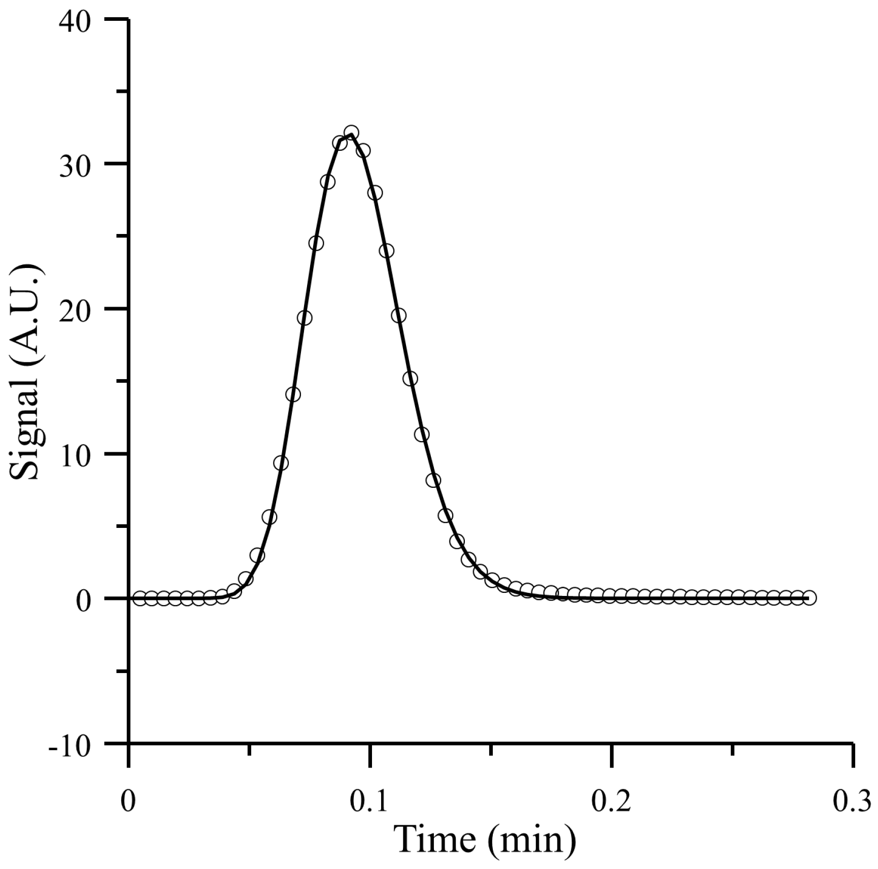
The extra-column effects can be taken into account assuming that the solute moves through the external tubing similarly to through the column, but without interacting with the stationary phase. Thus, the tubes can be divided into M plates as shown in Figure 2.

This involves a mass transfer process that can be described by the following system of equations.

$$\begin{array}{l}{a}_{1,\mathrm{ext}}^{(1)}=-{\mathsf{\tau }}_{\mathrm{ext}}{a}_{1,\mathrm{ext}}+d_{\mathrm{ext}}(a_{2,\mathrm{ext}}-a_{1,\mathrm{ext}})\\ ⋮\\ a_{i,\mathrm{ext}}^{(1)}=-{\mathsf{\tau }}_{\mathrm{ext}}(a_{i,\mathrm{ext}}-a_{i-1,\mathrm{ext}})+d_{\mathrm{ext}}(a_{i+1,\mathrm{ext}}-a_{i,\mathrm{ext}})-d_{\mathrm{ext}}(a_{i,\mathrm{ext}}-a_{i-1,\mathrm{ext}})\\ ⋮\\ a_{M,\mathrm{ext}}^{(1)}=-{\mathsf{\tau }}_{\mathrm{ext}}(a_{M,\mathrm{ext}}-a_{M-1,\mathrm{ext}})-d_{\mathrm{ext}}(a_{M,\mathrm{ext}}-a_{M-1,\mathrm{ext}})\end{array}$$

(31)

which would be added at the beginning of Equation System (29). The theoretical plate in the extra-column region has been considered to be different from the theoretical plate inside the column:

$${\mathsf{\tau }}_{\mathrm{ext}}=\frac{M}{t_{\mathrm{ext}}}=\frac{u_{\mathrm{ext}}}{H_{\mathrm{ext}}}=\frac{F}{V_{\mathrm{m},\mathrm{ext}}}$$

(32)

$$d_{\mathrm{ext}}=\frac{D}{H_{\mathrm{ext}}^2}$$

(33)

where H_ext is the extra-column plate height, t_ext the extra-column time, and D the apparent longitudinal diffusion that can be described by the Taylor-Aris regime if the capillary diameter is large enough [38].

Regardless the longitudinal diffusion, the extra-column peak shape according to this approach is similar to that given by Equation (3). Figure 3 shows the fitting to Equation (3) of an extra-column peak obtained for a probe compound (sulfamerazine), which is fairly satisfactory.

2.3. Peak Profile

The ordinary differential Equation System (29) is a first order system that can take the general form:

$$\frac{\mathrm{d}n}{\mathrm{d}t}=Qn$$

(34)

where n is a vector containing the solute moles in both mobile phase and stationary phase in each column plate, t is the time, and Q is a square matrix (2N × 2N) containing the mass transfer constants. The general solution for this system is given by:

$$n_i(t)={\displaystyle \sum _{j=1}^{2N}{z}_{ij}\frac{t^{m_j-1}}{(m_j-1)!}{e}^{{\lambda }_{j}t}}$$

(35)

where m_j are integers related to the multiplicity of the eigenvalues of matrix Q (m_j takes a value unity if the multiplicity is one). The peak profile function only has a simple form when the elution follows the Martin and Synge ideal conditions. In this case, matrix Q has only one eigenvalue with N multiplicity and the peak equation is that shown in Equation (3). With other assumptions, the complexity of the peak function is extraordinarily increased [10]. However, even assuming slow mass transfer, the peak equations tend to an almost Gaussian function (with very low asymmetry) if N is high enough.

Therefore, given the high number of theoretical plates and the complexity reached by matrix Q for complex cases, the peak equation (Equation (35)) lacks of practical value, being the study through the calculation of moments preferable.

2.4. Evaluation of Peak Profile Moments

2.4.1. General Method

As explained in previous work [10], obtaining an explicit equation for the peak profile is highly difficult or unfeasible. Therefore, we characterized the peaks through the calculation of the associated moments, following the procedure described below:

(i)

The equations describing the elution process (in this work, the sum of Equation Systems (31) and (29)) are first outlined.

(ii)

The system of differential equations is transformed to a system of algebraic equations in the Laplace space, which is a function of the variable r.

(iii)

The peak function is then obtained in the Laplace space (r-domain): F(r).

(iv)

To obtain the moments about the origin, the following property of the Laplace transformation is considered [10]:

$${\mu }_n={\displaystyle {\int }_0^{\infty }{t}^{n}f(t)\mathrm{d}t}={(-1)}^n\underset{r\to 0}{\lim }\frac{{\mathrm{d}}^{n}F(r)}{\mathrm{d}{r}^n}={(-1)}^{n}F{(r)}_{r=0}^{(n)}$$

(36)

(v)

For the moment of order n, the system of equations in the Laplace space describing the elution is derived n fold with regard to r. Then, it is solved to obtain the corresponding derivative after making r = 0 (see Equation (36)).

(vi)

The peak parameters are obtained from the moments about the origin.

Although the operations are simple and just consist in solving a linear equation system, the large number of implied equations makes the process rather complex. To follow it, it is interesting to understand the meaning of the derivatives at r = 0 in Equation (36). The derivative of order 0 is proportional to the amount of substance passing through the theoretical plate, the derivative of order 1 is proportional to the average time taken to cross the theoretical plate, and the derivative of order 2 is proportional to the average squared time to cross the theoretical plate.

2.4.2. Transformation of the System of Differential Equations into the Laplace Space

Obtaining the Laplace transform of the first-order Equation Systems (29) and (31) is rather simple. The Appendix of this work shows the whole process to calculate the first and second derivatives with regard to r. From Equation (30), the peak profile in the r-domain will be:

$$F(r)=\mathsf{\tau }{A}_N$$

(37)

where A_N is the variable in the Laplace domain associated to the mobile phase moles in the last theoretical plate. Taking into account Equation (36) and considering that τ is a constant parameter:

$${\mathsf{\mu }}_n={\left(-1\right)}^n\mathsf{\tau }{A}_{N(r=0)}^{(n)}$$

(38)

The peak position is given by the first moment about the origin:

$$\overline{t}=\frac{{\mu }_1}{{\mu }_0}=-\frac{A_{N(r=0)}^{(1)}}{A_{N(r=0)}}$$

(39)

The variance is given by the second-order moment about the mean:

$${\mathsf{\sigma }}^2=\frac{{\mathsf{\mu }}_2}{{\mathsf{\mu }}_0}-{\left(\frac{{\mathsf{\mu }}_1}{{\mathsf{\mu }}_0}\right)}^2=\frac{A_{N(r=0)}^{(2)}}{A_{N(r=0)}}-{\left(\frac{A_{N(r=0)}^{(1)}}{A_{N(r=0)}}\right)}^2$$

(40)

2.4.3. Solution for the Mean and Variance of the Peak Profile

The derivatives of the Laplace function associated to the last theoretical plate have been obtained using the approach described above, as shown in the Appendix. The derived equations are:

$$A_{N(r=0)}=\frac{a_0}{\mathsf{\tau }}$$

(41)

$$A_{N(r=0)}^{(1)}=-\frac{a_0}{\mathsf{\tau }{\mathsf{\tau }}_{\mathrm{ext}}}M-a_0\frac{1+k}{{\mathsf{\tau }}^2}N$$

(42)

$$\begin{array}{l}{A}_{N(r=0)}^{(2)}=\frac{a_0}{\mathsf{\tau }{\mathsf{\tau }}_{\mathrm{ext}}^2}(M^2+M)+2\frac{d_{\mathrm{ext}}}{\mathsf{\tau }{\mathsf{\tau }}_{\mathrm{ext}}^3}(M-1)a_0+2\frac{(1+k)}{{\mathsf{\tau }}^2{\mathsf{\tau }}_{\mathrm{ext}}}NM{a}_0\\ +\frac{{(1+k)}^2}{{\mathsf{\tau }}^3}(N^2+N)a_0+2(d_{\mathrm{m}}+k{d}_{\mathrm{s}})\frac{{(1+k)}^2}{{\mathsf{\tau }}^4}N{a}_0+2N\frac{a_0}{\mathsf{\nu }{\mathsf{\tau }}^2}k(1+k)\end{array}$$

(43)

By substituting Equations (41)–(43) in the corresponding equations (Equations (38)‒(40)), the different moments are obtained:

$${\mathsf{\mu }}_0=F_{(r=0)}^{(0)}=\mathsf{\tau }{A}_{N(r=0)}=a_0$$

(44)

which agrees with the characteristics of the Laplace transform and the fact that, along the chromatographic elution (where τ > d_m), all solute molecules cross the whole column.

The mean elution time is obtained from Equation (39):

$$\overline{t}=\frac{M}{{\mathsf{\tau }}_{\mathrm{ext}}}+\frac{N}{\mathsf{\tau }}(1+k)=t_{\mathrm{ext}}+t_0(1+k)=t_{\mathrm{ext}}+t_{\mathrm{col}}=t_{\mathrm{R}}$$

(45)

where t_ext is the extra-column time, t_col = t₀ (1 + k) is the column time, and t_R the experimental retention time. For this calculation, Equations (17) and (32) have been considered.

To calculate the variance, we will start from Equation (40), and operate considering Equations (41)‒(43):

$${\mathsf{\sigma }}^2=\frac{M}{{\mathsf{\tau }}_{\mathrm{ext}}^2}+2\frac{d_{\mathrm{ext}}}{{\mathsf{\tau }}_{\mathrm{ext}}^3}(M-1)+\frac{{(1+k)}^2}{{\mathsf{\tau }}^2}N+2(d_{\mathrm{m}}+k{d}_{\mathrm{s}})\frac{{(1+k)}^2}{{\mathsf{\tau }}^3}N+2N\frac{k(1+k)}{\mathsf{\nu }\mathsf{\tau }}$$

(46)

Taking into account Equations (17), (26), (32) and (33), the following results:

$${\mathsf{\sigma }}^2=\frac{t_{\mathrm{ext}}^2}{M}\left(1+2\frac{D}{H_{\mathrm{ext}}{u}_{\mathrm{ext}}}\frac{M-1}{M}\right)+\frac{t_{\mathrm{col}}^2}{N}\left(1+2\frac{D_{\mathrm{m}}+k{D}_{\mathrm{s}}}{Hu}+2\frac{k}{1+k}\frac{u}{H\mathsf{\nu }}\right)$$

(47)

This equation agrees with Equation (5) when t_ext = 0, D_m = 0, D_s = 0 and ν = ∞. The first term is the extra-column variance. Considering that in the extra-column capillary tubes, the axial dispersion should be controlled by the Taylor-Aris regime [38]:

$$D\equiv D_{\mathrm{m}}+\frac{r_{\mathrm{ext}}^2{u}_{\mathrm{ext}}^2}{48D_{\mathrm{m}}}=D_{\mathrm{m}}+w_{\mathrm{ext}}{u}_{\mathrm{ext}}^2$$

(48)

where r_ext is the radius of the extra-column tubing. Finally, the extra-column effect is given by:

$${\mathsf{\sigma }}_{\mathrm{ext}}^2=\frac{t_{\mathrm{ext}}^2}{M}\left(1+2\frac{D_{\mathrm{m}}}{H_{\mathrm{ext}}{u}_{\mathrm{ext}}}\frac{M-1}{M}+2\frac{w_{\mathrm{ext}}{u}_{\mathrm{ext}}}{H_{\mathrm{ext}}}\frac{M-1}{M}\right)$$

(49)

The column variance produced by a solute travelling in a unique path will be described by the second term in Equation (47), which could also include a term for considering the Taylor-Aris dispersion in the column:

$${\mathsf{\sigma }}_{\mathrm{col}}^2=\frac{t_{\mathrm{col}}^2}{N}\left(1+2\frac{D_{\mathrm{m}}+k{D}_{\mathrm{s}}}{Hu}+2\frac{k}{1+k}\frac{u}{H\mathsf{\nu }}+2\frac{w_{\mathrm{col}}u}{H_{}}\right)$$

(50)

However, owing to the small interstitial diameter within the column and the smaller linear velocity, this term would only be significant at high velocities, and will not be considered.

3. Experimental Section

3.1. Reagents and Columns

Five sulfonamides were used as probe compounds: sulfamerazine, sulfamethizole, sulfachloropyridazine, sulfisoxazole and sulfadimethoxine, purchased from Sigma (St. Louis, MO, USA), which were dissolved in a small amount of acetonitrile and diluted with water up to reach the concentrations of the stock and injected solutions (100 and 10 µg/mL, respectively), and stored in the darkness at 4 °C.

The mobile phase was prepared with 20% (v/v) HPLC-grade acetonitrile from Scharlau (Barcelona, Spain) and buffered at approximately pH 3 using 0.01 M sodium dihydrogen phosphate from Panreac (Barcelona, Spain) and HCl from Scharlau. Nanopure water obtained with a Barnstead purification system from Sybron (Boston, MA, USA) was used throughout. The mobile phase and the solutions of the probe compounds were filtered through 0.45 μm Nylon membranes with a diameter of 47 mm (Magna type) and 17 mm (Cameo type), respectively, from Osmonics (Herentals, Belgium).

Chromatographic analysis was carried out with a Spherisorb (150 mm × 4.6 mm ID) column with 5 μm particles from Scharlau. The column was protected with a pre-column of similar characteristics (30 mm × 4.0 mm).

3.2. Apparatus and Measurement of Peak Parameters

The HPLC system was equipped with the following modules from Agilent (Waldbronn, Germany): quaternary pump, autosampler, thermostated column compartment and UV-visible detector (Series 1200 and 1260). The signals were monitored at 254 nm. The flow rate was 1 mL/min and the dead time, 1.18 min. Dead time and extra-column contributions were measured by injecting a solution containing 20 μg/mL KBr from Acros Organics (Fair Lawn, NJ, USA).

The chromatographic system was controlled by a ChemStation from Agilent (B.04.03). The peak mean time and variance were calculated from the peak moments measured by numerical integration of experimental peaks using the Simpson rule. Data treatment was implemented in QB64.

The pH was measured with a potentiometer from Crison (Model MicropH 2002, Barcelona, Spain) and a combined glass electrode containing Ag/AgCl reference electrodes with 3.0 M KCl aqueous solution as salt bridge from Orion (Model 8102, Barcelona, Spain). The electrode was calibrated with aqueous buffers, and the pH of the mobile phases measured after the addition of the organic solvent.

4. Results and Discussion

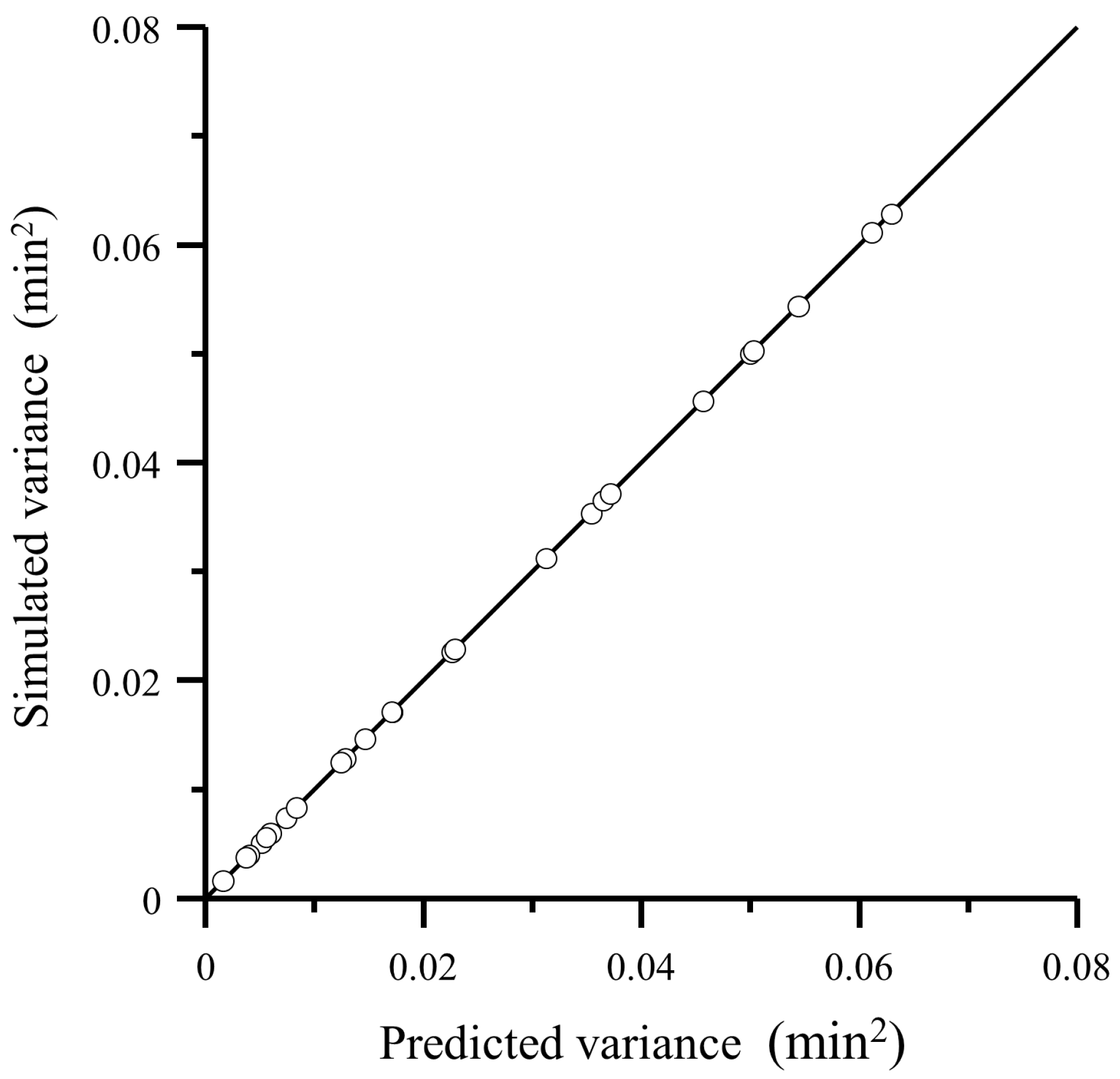
4.1. Comparison of the Proposed Model with a Simulation Approach

The proposed approach was checked by comparison with the profile obtained by simulation of the solute migration using the finite difference approach [18], dividing the process inside a theoretical plate in 100 time intervals. This was repeated for all theoretical plates up to achieve full elution from the column. The variance values calculated with the simulation approach and predicted with Equation (46) are compared in Figure 4 for hypothetical compounds exhibiting different retention times and assuming several values of column and extra-column theoretical plates, flow rate, mass transfer, and longitudinal diffusion. The high agreement between both approaches in different situations proves the validity of Equations (46) and (47).

Figure 5 depicts simulated peaks along with the corresponding Gaussian peaks, obtained using the peak profile parameters (mean time and variance) according to Equations (45) and (46). As observed, the agreement is highly satisfactory and the peaks were highly symmetrical, independently of the variation in mass transfer or diffusion (asymmetry values, measured as B/A at 10% peak high, were in the 1.04–1.09 range).

4.2. Comparison of Predicted Variance with Experimental Data

It is not possible to know the linear velocities needed in Equation (47), because the effective lengths are unknown. A transformation to volume and flow units is thus convenient, according to the following relationship:

$$u=F\frac{L}{V_0}=F\frac{L_{\mathrm{ext}}}{V_{\mathrm{ext}}}$$

(51)

The final equation, obtained by combination of Equations (49) and (50), would be:

$${\mathsf{\sigma }}_{\mathrm{V}}^2={\mathsf{\sigma }}^2{F}^2=A_{\mathrm{V}}+\frac{B_{\mathrm{V}}}{F}+C_{\mathrm{V}}F$$

(52)

where

$$A_{\mathrm{V}}=\frac{V_{\mathrm{ext}}^2}{M}+\frac{V_0^2}{N}{(1+k)}^2={\alpha }_0+{\alpha }_1{(1+k)}^2$$

(53)

$$B_{\mathrm{V}}=2\frac{D_{\mathrm{m}}{V}_{\mathrm{ext}}^3}{L_{\mathrm{ext}}^2}\frac{M-1}{M}+2\frac{D_{\mathrm{m}}+k{D}_{\mathrm{s}}}{L^2}{V}_0^3{(1+k)}^2={\mathsf{\beta }}_0+{\mathsf{\beta }}_{1}k+{\mathsf{\beta }}_2{k}^2+{\mathsf{\beta }}_3{k}^3$$

(54)

$$C_{\mathrm{V}}=2w_{\mathrm{ext}}{V}_{\mathrm{ext}}\frac{M-1}{M}+\frac{2}{\mathsf{\nu }}{V}_{0}k(1+k)={\mathsf{\gamma }}_0+{\mathsf{\gamma }}_{1}k(1+k)$$

(55)

Figure 6 shows the behavior of parameters A_V, B_V and C_V according to Equations (53)–(55). As observed in the figure, the parameters show the behavior predicted in the equations. Thus, parameters A_V and C_V are linear against (1 + k)² and k(1 + k), respectively, while parameter B_V gives rise to a third-order polynomial function against k. The quality of the fittings should be emphasized, especially for the C_V term, considering that there are other more complex contributions to the band broadening that have not been taken into account [38]. In addition, the diffusion constants and mass transfer may vary with the eluted solute. Finally, a similar linear behavior of parameter C_V with (1 + k)² could be found if the dispersion followed the Taylor-Aris regime.

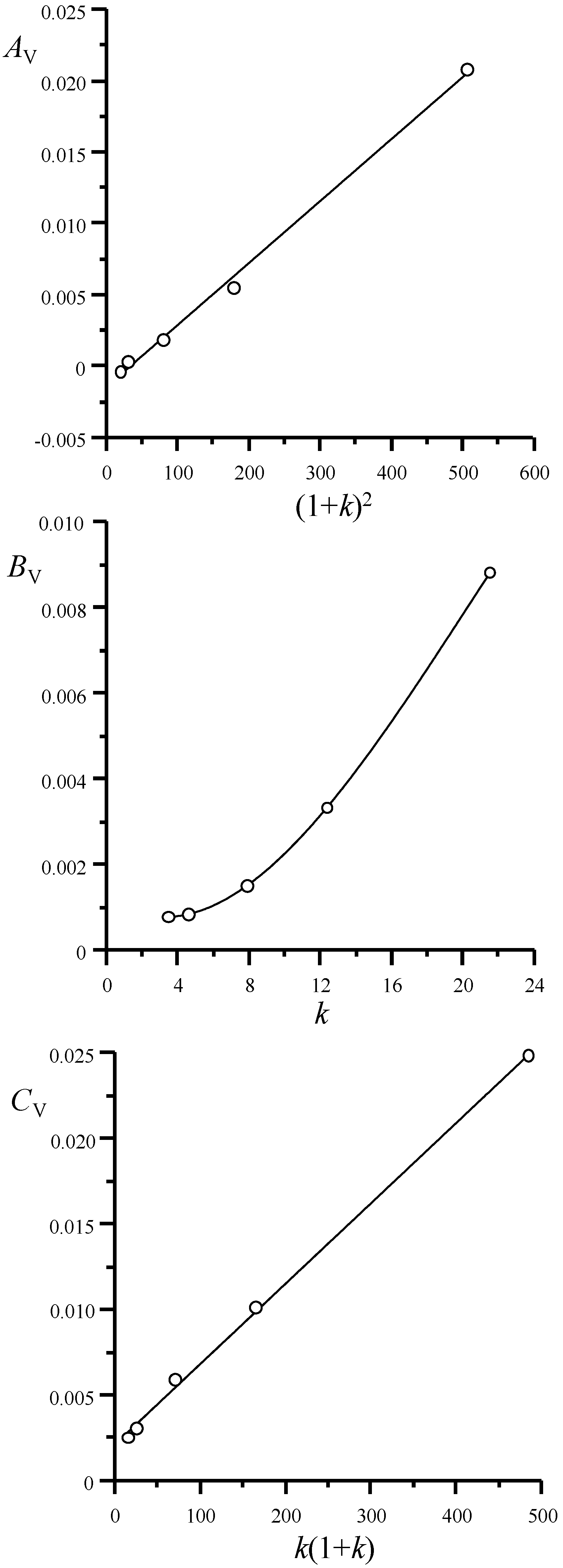
4.3. Variance Components

From Equation (47), we can see that in the elution process the sum of variances established in Equation (13) is fulfilled and taken as an initial premise to obtain the usual equations to calculate the theoretical plate. According to this point of view, the variance components come from the following sources:

(i)

Equilibrium between the mobile phase and stationary phase according to a Craig process:

$${\mathsf{\sigma }}_{\mathrm{eq}}^2=\frac{t_{\mathrm{col}}(t_{\mathrm{col}}-t_0)}{N}$$

(56)

(ii)

Convection or flow through the column:

$${\mathsf{\sigma }}_{\mathrm{conv}}^2=\frac{t_{\mathrm{col}}{t}_0}{N}$$

(57)

This variance is exclusively due to the flow, and can be obtained considering that it follows Equation (6), which describes the variance of a solute that does not interact with the stationary phase. Assuming that this broadening is only experienced by molecules found in the mobile phase:

$${\mathsf{\sigma }}_{\mathrm{conv}}^2=\frac{a^{*}}{a^{*}+b^{*}}\frac{t_{\mathrm{col}}^2}{N}=\frac{1}{1+k}\frac{t_{\mathrm{col}}^2}{N}=\frac{t_{\mathrm{col}}{t}_0}{N}$$

(58)

where a^* and b^* are the moles of solute at equilibrium in the mobile phase and stationary phase, respectively. Finally, the ideal variance for a column without slow mass transfer or diffusion will be:

$${\mathsf{\sigma }}_{\mathrm{elution}}^2=\frac{t_{\mathrm{col}}(t_{\mathrm{col}}-t_0)}{N}+\frac{t_{\mathrm{col}}{t}_0}{N}=\frac{t_{\mathrm{col}}^2}{N}$$

(59)

(iii)

Slow mass transfer between the phases:

$${\mathsf{\sigma }}_{\mathrm{mt}}^2=2\frac{t_{\mathrm{col}}}{\mathsf{\nu }}k$$

(60)

(iv)

Mobile phase diffusion:

$${\mathsf{\sigma }}_{\mathrm{diff},\mathrm{m}}^2=2D_{\mathrm{m}}\frac{t_{\mathrm{col}}^2{t}_0}{L^2}$$

(61)

(v)

Stationary phase diffusion:

$${\mathsf{\sigma }}_{\mathrm{diff},\mathrm{s}}^2=2k{D}_{\mathrm{s}}\frac{t_{\mathrm{col}}^2{t}_0}{L^2}$$

(62)

(vi)

Extra-column dispersion given by Equation (49) that includes convection, diffusion and dispersion due to the Taylor-Aris regime.

It is interesting to note that the components of band broadening due to mass transfer and diffusion do not depend on the theoretical plate height, but on the residence time inside the column.

4.4. Equation Describing the Theoretical Plate Height

The total variance is usually expressed in terms of the theoretical plate height, which includes all column band broadening factors. However, in the Martin and Synge elution model, the theoretical plate is a fixed parameter. Therefore, transforming Equation (47) to the usual terms, band broadening should be expressed as:

$$\frac{{\mathsf{\sigma }}^2-{\mathsf{\sigma }}_{\mathrm{ext}}^2}{{(t_{\mathrm{R}}-t_{\mathrm{ext}})}^2}L=H_{\mathrm{app}}=H+2\frac{D_{\mathrm{m}}+k{D}_{\mathrm{s}}}{u}+2\frac{k}{1+k}\frac{u}{\mathsf{\nu }}$$

(63)

Equation (63) gives an apparent value for the theoretical plate height (in the plate model H = L/N is a system constant). Therefore, the calculated theoretical plate (H_app) agrees with the real value only in the absence of longitudinal diffusion, multipath diffusion and slow mass transfer dispersion. In these conditions, as can be seen in Equation (10), the rate models would predict a null value for the band broadening. Thus, the extended plate approach and the rate models only agree when N tends to infinite. Equation (63) can be rewritten as:

$$H_{\mathrm{app}}=A+\frac{B}{u}+Cu$$

(64)

which agrees with the van Deemter equation except that the term A is associated to the dispersion due to convection. However, it can also be related to the particle diameter (d_p): (H = n_H × d_p, being n_H the number of particles inside a theoretical plate). Besides, other sources of dispersion independent of the flow (as the multipath dispersion) should be included in this term. On the other hand, the term C in Equation (63) seems also different from that in Equation (10). Taking into account that ν = s + m and k = m/s, the mass transfer term in Equation (63) may be expressed with regard to the retention factor as:

$$C=\frac{2}{\mathsf{\nu }}\frac{k}{1+k}=\frac{2}{s}\frac{k}{{(1+k)}^2}=\frac{2}{m}{\left(\frac{k}{1+k}\right)}^2$$

(65)

where each term assumes a constant kinetic parameter.

5. Conclusions

The original Martin and Synge approach has been extended to describe longitudinal diffusion in both mobile phase and stationary phase, slow mass-transfer and extra-column dispersion. To our knowledge, this is the first time the plate model has been solved including longitudinal diffusion in both phases, together with the slow mass transfer. Moreover, the extra-column dispersion has been included as a part of the dispersion model.

A systematic approach to obtain the moments of the elution profile applying the extended plate model has been developed. The final equation agrees with the van Deemter description for longitudinal diffusion in the mobile phase, and with the Knox equation, which also includes the diffusion in the stationary phase. The slow mass transfer results in a similar term to that in the van Deemter approach, but including a k/(1 + k) factor that fits better to the experimental data. The equations, expressed as a function of the theoretical plate height, provide an explanation for the three terms in the van Deemter equation. The term A is associated to the dispersion produced by the flow due to the mixing process inside each plate, and would only be null for N values tending to infinite. Other factors contributing to term A, such as the multipath dispersion, should be considered separately.

Simulated experiments showed that neither the slow mass transfer nor the longitudinal diffusion yield significant peak asymmetry. The plate model is assimilated to a kinetic mass transfer process coupling the various processes that take place both extra-column and inside the column. The proposed equation demonstrates the assumption of the sum of variances in the case of linear elution. Therefore, the plate model could be used to study separately each factor affecting the dispersion, adding in a further step each contribution to the final variance. The approach can be applied to study the factors affecting the elution process individually for educational purposes, only requiring knowledge on the solving of algebraic equations.

References

1. Martin, A.J.P.; Synge, R.L.M. A new form of chromatogram employing two liquid phases. Biochem. J. 1941, 35, 1358–1368. [Google Scholar] [CrossRef] [PubMed]
2. Martin, A.J.P.; Synge, R.L.M. Separation of the higher monoamino acids by counter-current liquid-liquid extraction: The amino-acid composition of wool. Biochem. J. 1941, 35, 91–121. [Google Scholar] [CrossRef] [PubMed]
3. Howard, G.A.; Martin, A.J.P. The separation of the C12-C18 fatty acids by reversed-phase partition chromatography. Biochem. J. 1950, 46, 532–538. [Google Scholar] [CrossRef]
4. Ettre, L.S. Obituary A.J.P. Martin (1910–2002). J. Chromatogr. A 2002, 972, 131–136. [Google Scholar]
5. Craig, L.C. Identification of small amounts of organic compounds by distribution studies: Separation by counter-current distribution. J. Biol. Chem. 1944, 155, 519–534. [Google Scholar] [CrossRef]
6. Williamson, B.; Craig, L.C. Identification of small amounts of organic compounds by distribution studies. V. Calculation of theoretical curves. J. Biol. Chem. 1947, 168, 687–697. [Google Scholar] [PubMed]
7. Felinger, A. Data Analysis and Signal Processing in Chromatography; Elsevier: Amsterdam, The Netherlands, 1998. [Google Scholar]
8. Said, A.S. Theoretical plate concept in chromatography. AIChE J. 1956, 2, 477–481. [Google Scholar] [CrossRef]
9. Said, A.S. Theoretical plate concept in chromatography: Part II. AIChE J. 1959, 5, 69–72. [Google Scholar] [CrossRef]
10. Baeza-Baeza, J.J.; García-Álvarez-Coque, M.C. A theoretical plate model accounting for slow kinetics in chromatographic elution. J. Chromatogr. A 2011, 1218, 5166–5174. [Google Scholar] [CrossRef] [PubMed]
11. Forbes, C.; Evans, M.; Hastings, N.; Peacock, B. Statistical Distributions, 4th ed.; Wiley: New York, NY, USA, 2011. [Google Scholar]
12. Giddings, J.C. The nature of eddy diffusion. Anal. Chem. 1966, 38, 490–491. [Google Scholar] [CrossRef]
13. Gritti, F.; Guiochon, G. Relationship between trans-column eddy diffusion and retention in liquid chromatography: Theory and experimental evidence. J. Chromatogr. A 2010, 1217, 6350–6365. [Google Scholar] [CrossRef] [PubMed]
14. Grinias, J.P.; Bunner, B.; Gilar, M.; Jorgenson, J.W. Measurement and modeling of extra-column effects due to injection and connections in capillary liquid chromatography. Chromatography 2015, 2, 669–690. [Google Scholar] [CrossRef]
15. Gritti, F.; Guiochon, G. On the extra-column band-broadening contributions of modern, very high pressure liquid chromatographs using 2.1 mm I.D. columns packed with sub-2 μm particles. J. Chromatogr. A 2010, 1217, 7677–7689. [Google Scholar] [CrossRef] [PubMed]
16. Miyabe, K.; Guiochon, G. Fundamental interpretation of the peak profiles in linear reversed-phase liquid chromatography. Adv. Chromatogr. 2000, 40, 1–113. [Google Scholar] [PubMed]
17. Guiochon, G.; Felinger, A.; Shirazi, D.G.; Katti, A.M. Fundamentals of Preparative and Nonlinear Chromatography; Academic Press, Elsevier: Amsterdam, The Netherlands, 2006. [Google Scholar]
18. Hao, W.; Di, B.; Chen, Q.; Wang, J.; Yang, Y.; Sun, X. Study of the peak variance in isocratic and gradient liquid chromatography using the transport model. J. Cromatogr. A 2013, 1295, 67–81. [Google Scholar] [CrossRef] [PubMed]
19. Felinger, A.; Guiochon, G. Comparison of the kinetic models of linear chromatography. Chromatographia 2004, 60, S175–S180. [Google Scholar] [CrossRef]
20. Czok, M.; Guiochon, G. The physical sense of simulation models of liquid chromatography: Propagation through a grid or solution of the mass balance equation. Anal. Chem. 1990, 62, 189–200. [Google Scholar] [CrossRef]
21. Gao, H.; Lin, B. A simplified numerical method for the general rate model. Comput. Chem. Eng. 2010, 34, 277–285. [Google Scholar] [CrossRef]
22. Câmara, L.D.T. Stepwise model evaluation in simulated moving-bed separation of ketamine. Chem. Eng. Technol. 2014, 37, 301–309. [Google Scholar] [CrossRef]
23. Van Deemter, J.J.; Zuiderweg, F.J.; Klinkenberg, A. Longitudinal diffusion and resistance to mass transfer as causes of non-ideality in chromatography. Chem. Eng. Sci. 1996, 5, 271–289. [Google Scholar] [CrossRef]
24. Hawkes, S.J. Modernization of the Van Deemter equation for chromatographic zone dispersion. J. Chem. Educ. 1983, 60, 393–398. [Google Scholar] [CrossRef]
25. Golshan-Shirazi, S.; Guiochon, G. Review of the various models of linear chromatography and their solutions. In Theoretical Advancement in Chromatography and Related Separation Techniques; Dondi, F., Guiochon, G., Eds.; NATO ASI Series; Kluver Academic Publishers: Berlin, Germany, 1992; Volume 383, pp. 61–92. [Google Scholar]
26. Giddings, J.C.; Eyring, H. A molecular dynamic theory of chromatography. Anal. Chem. 1955, 59, 416–421. [Google Scholar] [CrossRef]
27. Felinger, A. Molecular dynamic theories in chromatography. J. Chromatogr. A 2008, 1184, 20–41. [Google Scholar] [CrossRef] [PubMed]
28. Chen, Y. The statistical theory of linear capillary chromatography with uniform stationary phase. J. Chromatogr. A 2007, 1144, 221–244. [Google Scholar] [CrossRef] [PubMed]
29. Tijssen, R. The mechanism and importance of zone spreading. In Handbook in HPLC; Kaltz, E., Eksteen, R., Schoenmakers, P., Miller, N., Eds.; Marcel Dekker: New York, NY, USA, 1998. [Google Scholar]
30. Gritti, F.; Guiochon, G. Mass transfer kinetics, band broadening and column efficiency. J. Chromatogr. A 2012, 1221, 2–40. [Google Scholar] [CrossRef] [PubMed]
31. Miyabe, K. Moment analysis of chromatographic behavior in reversed-phase liquid chromatography. J. Sep. Sci. 2009, 32, 757–770. [Google Scholar] [CrossRef] [PubMed]
32. Knox, J.H.; Scott, H.P. B and C terms in the Van Deemter equation for liquid chromatography. J. Chromatogr. 1983, 282, 297–313. [Google Scholar] [CrossRef]
33. Gritti, F.; Guiochon, G. General HETP equation for the study of mass-transfer mechanisms in RPLC. Anal. Chem. 2006, 78, 5329–5347. [Google Scholar] [CrossRef] [PubMed]
34. Usher, K.M.; Simmons, C.R.; Dorsey, J.G. Modeling chromatographic dispersion: A comparison of popular equations. J. Chromatogr. A 2008, 1200, 122–128. [Google Scholar] [CrossRef] [PubMed]
35. Knox, J.H. Band dispersion in chromatography: A new view of A-term dispersion. J. Chromatogr. A 1999, 831, 3–15. [Google Scholar] [CrossRef]
36. Knox, J.H. Band dispersion in chromatography: A universal expression for the contribution from the mobile zone. J. Chromatogr. A 2002, 960, 7–18. [Google Scholar] [CrossRef]
37. Desmet, G.; Broeckhoven, K.; de Smet, J.; Deridder, S.; Baron, G.V.; Gzil, P. Errors involved in the existing B-term expressions for the longitudinal diffusion in fully porous chromatographic media: Part I: Computational data in ordered pillar arrays and effective medium theory. J. Chromatogr. A 2008, 1188, 171–188. [Google Scholar] [CrossRef] [PubMed]
38. Datta, S.; Ghosal, S. Characterizing dispersion in microfluidic channel. Lap Chip 2009, 9, 2537–2550. [Google Scholar] [CrossRef] [PubMed]
Figure 1. Kinetic representation of the elution inside the column as a combination of mass transfer processes from plate to plate (see Glossary for symbol explanation).
Separations 03 00011 g001
Figure 2. Kinetic representation of the extra-column mass transfer (see Glossary for symbol explanation).
Separations 03 00011 g002
Figure 3. Extra-column experimental peak for sulfamerazine (symbols), compared with that predicted according to the plate model (Equation (3)) (solid line). Peak eluted using 1 mL/min flow rate and 20% acetonitrile. A.U. is arbitrary units.
Separations 03 00011 g003
Figure 4. Comparison of the calculated variance using the simulation approach with that predicted with Equation (46) for several elution conditions, changing N (in the range 500–2000), M (5–20), τext (50–400), dext (0.02–0.375), τ (500–2000), dm (20–400), ds (2–40), ν (1000–5000), and k (0–4).
Separations 03 00011 g004
Figure 5. Comparison of numerically simulated peaks (symbols) obtained by solving the differential system composed by Equation Systems (31) and (29) with Gaussian peaks (lines) obtained with the retention time and variance calculated with Equations (45) and (46) for a peak described by the following data: k = 3, t0 = 1.0, text = 0.1, M = 10, and from top to bottom: (◊) N = 2000, dext = 0.0222, dm = 80, ds = 8, ν = 5000; (○) N = 2000, dext = 0.111, dm = 400, ds = 40, ν = 2500; (□) N = 1000, dext = 0.111, dm = 100, ds = 10, ν = 1500. A.U. is arbitrary units.
Separations 03 00011 g005
Figure 6. Behavior of parameters AV, BV and CV calculated according to Equations (53)–(55). The plotted values were obtained by the non-linear fitting to Equation (52) of the experimental variances for the five sulfonamides eluted at several flow rates.
Separations 03 00011 g006