Global Supervisory Structure for Decentralized Systems of Flexible Manufacturing Systems Using Petri Nets

Abstract

Decentralized supervisory structure has drawn much attention in recent years to address the computational complexity in designing supervisory structures for large Petri net model. Many studies are reported in the paradigm of automata while few can be found in the Petri net paradigm. The decentralized supervisory structure can address the computational complexity, but it adds the structural complexity of supervisory structure. This paper proposed a new method of designing a global controller for decentralized systems of a large Petri net model for flexible manufacturing systems. The proposed method can both reduce the computational complexity by decomposition of large Petri net models into several subnets and structural complexity by designing a global supervisory structure that can greatly reduce the cost at the implementation stage. Two efficient algorithms are developed in the proposed method. Algorithm 1 is used to compute decentralized working zones from the given Petri net model for flexible manufacturing systems. Algorithm 2 is used to compute the global controller that enforces the liveness to the decentralized working zones. The ring assembling method is used to reconnect and controlled the working zones via a global controller. The proposed method can be applied to large Petri nets size and, in general, it has less computational and structural complexity. Experimental examples are presented to explore the applicability of the proposed method.

1. Introduction

Due to the complexity of flexible manufacturing systems in the recent years, decentralized systems control has drawn much attention worldwide by the researchers in the area of the discrete event systems. Large-scale discrete event systems (DES) are modeled through the composition of many smaller subsystems representing shared resources by the concurrent operations. The controlled of large-size flexible manufacturing systems is tedious and time-consuming, perhaps it required huge memory space due to a large number of its state space. Moreover, the analysis of complex systems is very complicated and sometimes remains non-deterministic polynomial time (NP-hard). To reduce the computational complexity and required memory space for the analysis and control of large flexible manufacturing systems, we decomposed the systems into several working zones (i.e., several sub-problems).

Several methods are developed in the literature to analyze the decentralized systems of DES-based on the system applications. Most of the methods focus on the design of a decentralized controller (i.e., modular controller) to supervise the operations of the DES. The DES find application in the areas of automation [1,2], software development [3], computer engineering [4,5], communication systems [6], flexible manufacturing system [7,8] and transportation networks [9]. The main challenges of the study of DES are the occurrence of deadlocks. Deadlocks can occur due to excessive use of shared resources in the systems, which degrade the system performance of DES [10,11,12,13,14,15,16,17]. Three main tools exist to design a decentralized supervisory structure for DES, namely, they are; graph theory [2,5,15,16], automata [18,19,20,21,22] and Petri nets [14,16,23,24,25,26,27]. This paper focuses on the design of a global supervisory structure for decentralized systems using the Petri nets paradigm.

In a Petri net paradigm, forbidden states are often specified by linear constraints. The concept of generalized mutual exclusion constraints (GMECs) is often used to analyze and construct a supervisory structure that enforces the liveness of the DES [25,27,28]. The emergence of large Petri nets model for flexible manufacturing systems motivates the research to decompose the systems in a systematic method. The work of Li in [29] developed a divide and conquer method to control the deadlocks. The developed method is used to decompose the Petri net model into smaller subnets, in such a way that the decomposition is done via resource transition circuits. Control places are designed using siphon techniques for the decomposed subnets. This adds the structural complexity to the size of the supervisory structure. Uzam et al. modified the divide and conquer method in [30] via an iterative decomposition of the Petri net model. At each iteration, control places are designed for the decomposed subnets using reachability techniques. The method suffers from the computational complexity since it involved the computation of the reachability graph at each iteration.

A modular supervisory scheme for modeling and synthesis of supervisory agents using a Petri net model is developed in [4]. These modular supervisors are conceived as operating independently, each exercising control to satisfy its own specification. However, when all the modular supervisors operate concurrently, they may result in conflict. To reduce the computational complexity for the design of the supervisory structure, the work presented in [31] proposed two methods for the decentralized supervisory structure. The first method considers the design of decentralized supervisory structure using communication while assuming that all the transitions in the Petri net model are observable and controllable. The second method considers the transformation of constraints that is not d-admissible in the design of the decentralized supervisory structure with no communications. The solution is obtained by solving integer linear programming (ILPP). The first method allows more reachable states than the second method due to the advantage of unrestricted communications. Generating and solving integer linear programming problem (ILPP) is computationally complex [32,33,34,35] and can limit the application of the developed methods.

It is generally known that computation of a reachability graph is computationally complex and sometimes NP-hard. To avoid the computation of the reachability graph, the authors in [17] developed a new method of decentralized supervisory control for communication systems using a Petri nets paradigm. The communication among the decentralized subnets are enforced in a centralized environment. Ye et al. in [28] extended the works to flexible manufacturing systems that emphasized the efficiency of the decomposition of Petri nets for flexible manufacturing systems. The developed method designs a decentralized supervisory structure without transforming the inadmissible constraints to admissible constraints. The communication constraints are incorporated between the decentralized subnets. The decentralized supervisory structure is usually associated with structural complexity, which require huge costs in the implementation stage. The computational and structural complexity is addressed in the proposed paper. The former is achieved by decomposition of Petri nets into a several subnets model while the latter is addressed using a global supervisory structure.

The study of [36] proposed a decomposition of a Petri net model through the use of local invariants (place and transition invariants) computation since it is well-known that the invariants can help to prove structural properties of Petri nets, i.e., boundedness, reversibility, liveness, and safeness. This proposed paper utilized the use of P-invariants in the decomposition of a large Petri net model and the operation for each decentralized subnet can be monitored using the global controller unlike the work of Bourjij et al. in [36] that the global solution can only be found by the concatenation of the subnets that has the same coupling power.

In this paper, we proposed a new method to design a global supervisory structure of the decentralized systems using Petri nets for flexible manufacturing systems. First, a subnet is computed from the given Petri net model for a flexible manufacturing system. Second, the subnet model is split into several decentralized working zones. The main contributions of the proposed paper are summarized as follows: (i) two efficient algorithms are developed, the first algorithm is used to compute the decentralized working zones from the subnet model, while the second algorithm is used to compute the global controller; (ii) the proposed method can reduce the computational and structural complexity through the use of global supervisory structure and (iii) the proposed method can be applied to a complex system for the computation of the supervisory structure.

The ring assembling is used to reconnect and control the working zones via a global controller. The global controller is computed and added to the decentralized working zones. When all the decentralized working zones are reconnected via a global controller, the resulting Petri net model is live maximally permissive behavior. Several experimental examples are used to explore the applicability of the proposed method.

The remainder of this paper is organized as follows. Formal descriptions of Petri nets and notations used in this paper are presented in Section 2. Section 3 provides the detail ideas for the computation of decentralized working zones. Design of a global controller is presented in Section 4. Experimental examples are provided in Section 5. Discussions are presented in Section 6. Finally, Section 7 concludes this paper.

2. Preliminaries

A Petri net is a four-tuple $N=(P,T,F,W)$, where P and T are finite and non-empty sets. P is a set of places and T is a set of transitions with $P\cap T=\varnothing$. $F\subseteq (P\times T)\cup (T\times P)$ is called a flow relation of the net, represented by arcs with arrows from places to transitions or from transitions to places. Places are graphically represented by circles while transitions by bars or square boxes. $W:(P\times T)\cup (T\times P)\to \mathbb{N}$ is a mapping that assigns a weight to an arc: $W(x,y)>0$ if $(x,y)\in F$, and  $W(x,y)=0$, otherwise, where $(x,y)\in (P\times T)\cup (T\times P)$ and $\mathbb{N}$ is the set of non-negative integers. $N=(P,T,F,W)$ is said to be ordinary, denoted as $N=(P,T,F)$, if $\forall f\in F$, $W\left(f\right)=1$. Let $x\in P\cup T$ be a node in $N=(P,T,F,W)$.

A marking of a Petri nets N describes the current state of the system. $M\left(p\right)$ denotes the number of tokens in place p. The presence of token in the Petri net structure makes the system to be dynamic. It is essential to track the places that are marked at each reachable marking. A place p is said to be marked at a marking M if $M\left(p\right)>0$. Usually, we express the markings and vectors as a formal sum notation or multiset for easy representation i.e., ${\sum }_{p\in P}M\left(p\right)p$. Let us consider a simple example, assuming we have a net system with places $p_1$ to $p_7$ formally represented as $P=\{p_1,\cdots ,p_7\}$. If we have a marking that has one token in place $p_3$ and two tokens in places $p_2$ and $p_5$, respectively, using multiset notation, the marking can be written as $2p_2+p_3+2p_5$ instead of $\left(0210200\right)$. In summary, a marking $\left(M\right)$ of $(N,M_0)$ is a mapping from P to N.

Let us assume $t\in T$ to be a transition in the Petri nets N. At any marking M, transition t is enabled if $\forall p\in {}^{•}t$, $M\left(p\right)\ge W(p,t)$. For  easier representation and without any ambiguity, it can be denoted as $M[t\rangle$. If the enable transition is fired, it leads the system into new reachable marking $M^{\prime }$. Formally, the tokens at each place in the new reachable marking can be tract as $\forall p\in P,M^{\prime }\left(p\right)=M\left(p\right)-W(p,t)+W(t,p)$ and this can be denoted as $M[t\rangle M^{\prime }$ in short.

Suppose that x is a node in the Petri net model i.e., $x\in P\cup T$. The input (preset) of x is expressed as ${}^{•}x=\{y\in P\cup T\mid (y,x)\in F\}$ and its output (postset) is expressed as $x^{•}=\{y\in P\cup T\mid (x,y)\in F\}$. The Petri net structure can be represented in matrix form and is called an incidence matrix. An incidence matrix is obtained from the input and output matrices. The input incidence matrix is defined as $\left[D^{-}\right]=W(p,t)$ and the output incidence matrix is defined as $\left[D^{+}\right]=W(t,p)$. Therefore, the incidence matrix of the net is expressed as $\left[D\right]=\left[D^{+}\right]-\left[D^{-}\right]$. The incidence vector for a place p (transition t) in the raw (column) incidence matrix can be represented as $\left[D\right](p,·)$ ($\left[D\right](·,t)$).

A Petri net model $(N,M_0)$ is said to be in a deadlock state when none of its transitions can be enabled at a marking M, i.e., $\nexists t\in T$, $M[t\rangle$ holds. A  Petri net model is deadlock free when some of the reachable states can not be observed. In other words, a deadlock free is called live-lock and can be expressed as $\forall M\in R(N,M_0)$, $\exists t\in T$, $M_0[t\rangle$. $(N,M_0)$ is said to be live if all its reachable states can return to its initial marking $M_0$. Mathematically, it can be expressed as $(N,M_0)$ being live if $\forall M\in R(N,M_0)$, $\forall t\in T$, $\exists M^{\prime }\in R(N,M)$, $M^{\prime }[t\rangle M_0$. Let M and $M^{\prime }$ be two markings in $R(N,M_0)$. M A-covers $M^{\prime }$ if $\forall p\in P_A$, $M\left(p\right)\ge M^{\prime }\left(p\right)$, which is denoted as $M\left(p\right){\ge }_A{M}^{\prime }\left(p\right).$

Let $\sigma$ be a transition sequence. The Parikh vector of $\sigma$, denoted by $\overrightarrow{\sigma }$, is a column vector, represented by $\overrightarrow{\sigma }$=$[\#\sigma \left(t_1\right),\#\sigma \left(t_2\right)$, $\dots ,\#\sigma \left(t_{\left|T\right|}\right){]}^T$, where $\#\sigma \left(t_i\right)$ denotes the number of occurrences of $t_i$ in $\sigma$. $\sigma \ast$ denote the set of all firing sequence in $(N,M_0)$. The notation $\xi \left({\sigma }^{\ast }\right)$ represents the vector firing sequence ${\sigma }^{\ast }$ in $(N,M_0)$ mapping from $(N,M_0)$ to its decentralized subnet. A P-vector is a column vector $I:$ $P\to \mathbb{Z}$, indexed by P, where $\mathbb{Z}=\{\dots ,-2,-1,0,1,2,\dots \}$. A P-vector I is a place invariant if $I\ne \mathbf{0}$ and $I^T\left[D\right]={\mathbf{0}}^T$. A T-vector is a column vector $H:T\to \mathbb{Z}$ indexed by T. A T-vector H is a transition invariant if $\left[D\right]H=$0 and $H\ne$0. The  support of a place (transition) invariant $I\left(H\right)$ is denoted by $\left|\right|I\left|\right|=\left\{p\right|I\left(p\right)\ne 0\}$ $\left(\right|\left|H\right||=\{t\left|H\right(t)\ne 0\})$. Let ${\mathbb{N}}^{+}$ denote the set of positive integers.

3. Petri Net Model with S${}^3$PR

Systems of simple sequential processes with resources (S${}^3$PR) are extensively used and adopted in the analysis of FMSs [27,37,38]. This paper considers an S${}^3$PR class of Petri nets for flexible manufacturing systems.

Definition 1.

A system of simple sequential processes with resources (S${}^3$PR) is a Petri net $N=(P,T,F)$, satisfying [37]:

1. 

$P=P_A\cup P_R\cup P^0$ is a partition of places with $P_A\cap P_R=\varnothing$, $P_A\cap P^0=\varnothing$, and $P_R\cap P^0=\varnothing$;

(a) 

$p_i^0$ is called the process idle place of $N_i$. Elements in $P_A^i$ and $P_R^i$ are called operation and resource places;

(b) 

$P_A^i\ne \varnothing$; $P_R^i\ne \varnothing$; $p_i^0\in P^0$; $(P_A^i\cup \left\{p_i^0\right\})\cap P_R^i=\varnothing$;

(c) 

$\forall p\in P_A^i$, $\forall t{\in }^{•}p$, $\forall t^{\prime }\in p^{•}$, $\exists r_p\in P_R^i$, ${}^{•}t\cap P_R^i=t^{\prime •}\cap P_R^i=\left\{r_p\right\}$;

(d) 

$\forall r\in P_R^i$, ${}^{••}r\cap P_A^i=r^{••}\cap P_A^i\ne \varnothing$, ${}^{•}r\cap r^{•}=\varnothing$;

(e) 

${}^{••}\left(p_0^i\right)\cap P_R^i={\left(p_0^i\right)}^{••}\cap P_R^i=\varnothing$;

2. 

$T={\bigcup }_{i=1}^m{T}_i$, with $T_i\cap T_j=\varnothing$ for all $i\ne j$, is a set of transitions;

3. 

$N_i$ is a strongly connected state machine, where $N_i=(P_A^i\cup \left\{p_i^0\right\},T_i,F_i)$ is the resulting net after the places in $P_R^i$ and related arcs are removed from $N_i$;

4. 

Any two $N_i$ are composable when they share a set of common places. Every shared place must be a resource place.

5. 

For $p\in P_A$, ${}^{••}\left(p\right)\cap P_R=\left\{r_p\right\}$ where resource place $r_p$ is called the resource used by p.

Definition 2.

Let $(N,M_0)$ be the Petri net model with $N=(P,T,F)$, where $P=P_A\cup P_R\cup P^0$. $(N^{\prime },M_0)$ is said to be a subnet of $(N,M_0)$ with $N^{\prime }=(P^{\prime },T^{\prime },F^{\prime })$ if $P^{\prime }=P\backslash P^0$, $T^{\prime }=T$, $F^{\prime }=F\backslash Q$. $Q\subseteq (P^0\times T)\cup (T\times P^0)$ is called a flow relation of the net, represented by an arc with an arrow from idle places to transitions or transitions to idle places.

Definition 3.

Resource r is said to be shared if $\exists p,p^{\prime }\in \left(\right||I_r\left|\right|\backslash \left\{r\right\})$, $p\in P_{Ai}$, $p^{\prime }\in P_{Aj}$, $i\ne j$. Let the shared resource place denoted by r in $(N,M_0)$.

Definition 4.

Let $t\in T$ be the transition in $(N^{\prime },M_0)$. Transition t is said to be source transition if $|t^{•}|=1$ and is said to be sink transition if $|{}^{•}t|=1$. Let $t^s$ denote the source transition and $t^c$ denote the sink transition. The sets of source and sink transition are denoted as $\vartheta =\{t\mid t\in T,|t^{•}|=1\}$ and $\mathsf{\Psi }=\{t\mid t\in T,|t^{•}|=1\}$,  respectively.

Property 1.

Every concurrent process has at least one source and sink transitions in $(N,M_0)$.

3.1. Decentralization of FMS into Working Zones

The analysis of a complex Petri net model for a flexible manufacturing system is hard and time-consuming if it’s not NP-hard. The complex system can be addressed by dividing it into several decentralized problems (subnet).

Definition 5.

A subnet of a Petri net model is called a working zone denoted by $Z=(P^q,T^q,F^q)$ if it satisfies the following:

• $P^q=\parallel I_r\parallel$, $P^q=P_A^q\cup P_R^q$ is a partition of places with $P_A^q\cap P_R^q=\varnothing$. $P_A^q$ and $P_R^q$ is the set of activity and resource places, respectively;
• $T^q=\{t\mid t\in T^{\prime },{}^{•}\parallel I_r\parallel \cup \parallel I_r{\parallel }^{•}\}$ is the set of transition associated with the minimal P-semiflow;
• $\forall t\in T^{\prime }{,|}^{•}t|=|t^{•}|=1$ is a state machine;
• $F^q\to (P^q\times T^q)\cup (T^q\times P^q)$ is a flow relation simply represented by directed arcs;
• $\exists r\in P_R^{\prime }$, then $M\left(r\right)\ge 1$;
• Z is strongly bounded.

Suppose that we have $N^{\prime }=(P^{\prime },T^{\prime },F^{\prime })$ as a subnet from $(N,M_0)$ with $N=(P,T,F)$. $N^{\prime }$ consists of a set of a decentralized working zone ${\Im }_1=(P_1^q,T_1^q,F_1^q)$, ${\Im }_2=(P_2^q,T_2^q,F_2^q),\cdots$, and ${\Im }_{\ell }=(P_{\ell }^q,T_{\ell }^q,F_{\ell }^q)$ such that $P^{\prime }=P_1^q\cup P_2^q\cup \cdots \cup P_{\ell }^q$, $T^{\prime }=T_1^q\cup T_2^q\cup \cdots \cup T_{\ell }^q$, and $F^{\prime }=F_1^q\cup F_2^q\cup \cdots \cup F_{\ell }^q$. A transition $t\in T^{\prime }$ is a common transition if t belongs to ${\Im }_i$ and ${\Im }_j$ in $N^{\prime }$, $i,j\in \{1,2,\cdots ,\ell \}$ and $i\ne j$. Let $T_d\subseteq T^{\prime }$ denote a set of common transitions from $N^{\prime }$. With no ambiguity and easy representation, $\forall t\in T_d$, t can be rewritten as $t^{\prime }$ belongs to ${\Im }_i$ and $t^{″}$ belongs to ${\Im }_j$, where $t^{\prime },t^{″}$ s.t. $[t\rangle$ condition. Suppose that ${\Im }_z=(P_z^q,T_z^q,F_z^q)$ is a decentralized working zone from $N^{\prime }$, where $z\in \{1,\cdots ,\ell \}$ and ℓ is the number of working zones. $D_z$ is the incidence matrix of ${\Im }_z$ and each working zone can be represented as:

$$\forall t_j\in T_z^q,\mid \sum _{1\le i\le n,1\le j\le m}{D}_z(p_i,t_j)\mid \le 1.$$

(1)

The places of each decentralized working zone form the support of P-invariants and can be represented as a multiset

$$\parallel I\parallel =\sum _{i=1}^n{p}_i\ge 1,$$

(2)

where $n=|P_z^q|$ and $m=|T_z^q|$. Let $t_i\in T_z^{\prime }$, $i\in \{1,\cdots ,m\}$ be the transitions associated with the places in the P-invariants. All places in the support of P-invariants are connected to its corresponding transitions as

$$\forall i\in \{1,\cdots ,n\},\forall j\in \{1,\cdots ,m\},\exists p_i\in P_z^q,\exists t_j\in T_z^q,(p_i\times t_j)\cup (t_j\times p_i).$$

(3)

Let $D^{\prime }$ be the incidence matrix of the subnet model, and I be the P-invariant in the decentralized working zone. Each decentralized working zone should satisfy Equation (4),

$${}^{•}\parallel I\parallel ={\parallel I\parallel }^{•},I^T\left[D^{\prime }\right]=0^T.$$

(4)

Every working zone should contain at least one token after the decentralization, which implies that there exists at least one resource place in each decentralized working zone being marked at the initial marking $M_0$, i.e., for every ${\Im }_z$, $z\in \{1,\cdots ,\ell \}$

$$\exists r^s\in P_z^q,M\left(r^s\right)\ne 0.$$

(5)

Theorem 1.

Let $N^{\prime }=\{P^{\prime },T^{\prime },F^{\prime }\}$ be a subnet of $(N,M_0)$. $N^{\prime }$ can be decentralized into minimal working zones via Algorithm 1.

Algorithm 1 Decentralization of an FMS into working zones

Require: Petri net model of an FMS structure suffering from deadlock Ensure: Decentralized working zones   1: Compute the subnet model $(N^{\prime },M_0)$ from $(N,M_0)$ using Definition 2   2: Compute the minimal P-invariant $I_i$ in $(N^{\prime },M_0)$   3: Compute the support of minimal P-invariant $\parallel I_i\parallel$ from $(N^{\prime },M_0)$   4: $i\in \{1,2,\cdots ,n\}$, $/\ast n$ is the number of $\parallel I_i\parallel$ in $(N^{\prime },M_0)$$\ast /$   5: while$i\le n$do   6:     if $(\parallel I\parallel$ satisfied equ. 1–5) then   7:         Compute $T_i^q$ from $N^{\prime }$ using Definition 5   8:         Compute $T_d^i=T_i^q\cap T^{\prime }$   9:         Remove $Z_i=(P_i^q,T_i^q,F_i^q)$ from $N^{\prime }$, $P_i^q\subseteq \parallel I_i\parallel$ 10:         $P^{\prime }=P^{\prime }\backslash \parallel I_i\parallel$ 11:         $T^{\prime }\cup T_d^i=T^{\prime }\backslash T_i^q$ 12:         $F^{\prime }=F^{\prime }\backslash F_i^q$         $/\ast$ $T_d$ is the set of common transition between the two successive $Z_i\ast /$ 13:         endif 14:     $N^{\prime }=(P^{\prime },T^{\prime },F^{\prime })$ 15:     $i=i+1$ 16: end 17: Output the decentralized working zones

Proof. 

According to Definition 5, if $P^{\prime }\backslash P_A^{\prime }\ne \varnothing$, at least one share resource place (i.e., $\exists r\in P_R^{\prime }$) therefore exists in $(N^{\prime },M_0)$. It is obvious that any shared resource place for a Petri net model of an FMS forms a minimal P-semiflow $\parallel I_r\parallel$ such that $\left\{r\right\}=\parallel I_r\parallel \backslash P_A^{\prime }$, $P_A^{\prime }\in P^{\prime }$. Therefore, each minimal P-semiflow can satisfy Equations (1)–(5) of Algorithm 1 and hence the theorem holds. □

Theorem 2.

Let $(N^{\prime },M_0)$ be a system with $N^{\prime }=(P^{\prime },T^{\prime },F^{\prime })$ and ${\Im }_i$ be decentralized subnet from $N^{\prime }$, $i\in \{1,\cdots ,\ell \}$, where ℓ is the number of decentralized working zones. Let ${\sigma }^{\ast }$ and ${\sigma }_i^{\ast }$ denote all the transition firing sequences in $N^{\prime }$ and ${\Im }_i$, respectively. ${\xi }_i\left({\sigma }^{\ast }\right)={\sigma }_i^{\ast }$ if and only if for any two working zones ${\Im }_i$ and ${\Im }_j$ satisfied $T_i^{\prime }\cap T_i^{\prime }\ne \varnothing$, ${\sigma }_i^{\ast }{\mid }_{T_i\cap T_j}={\sigma }_j^{\ast }{\mid }_{T_i^{\prime }\cap T_j^{\prime }}$, for $i,j\in \{1,\cdots ,\ell \}$ [28].

To minimize space and redundancy, we can refer the reader to the work of [28] for the proof of Theorem 2. According to Theorem 2, both the structural and dynamic properties of subnet with that of decentralized systems are preserved and equivalence for any transition firing sequence from decentralized working zones that can be mapped into a subnet model.

3.2. Demonstrated Example

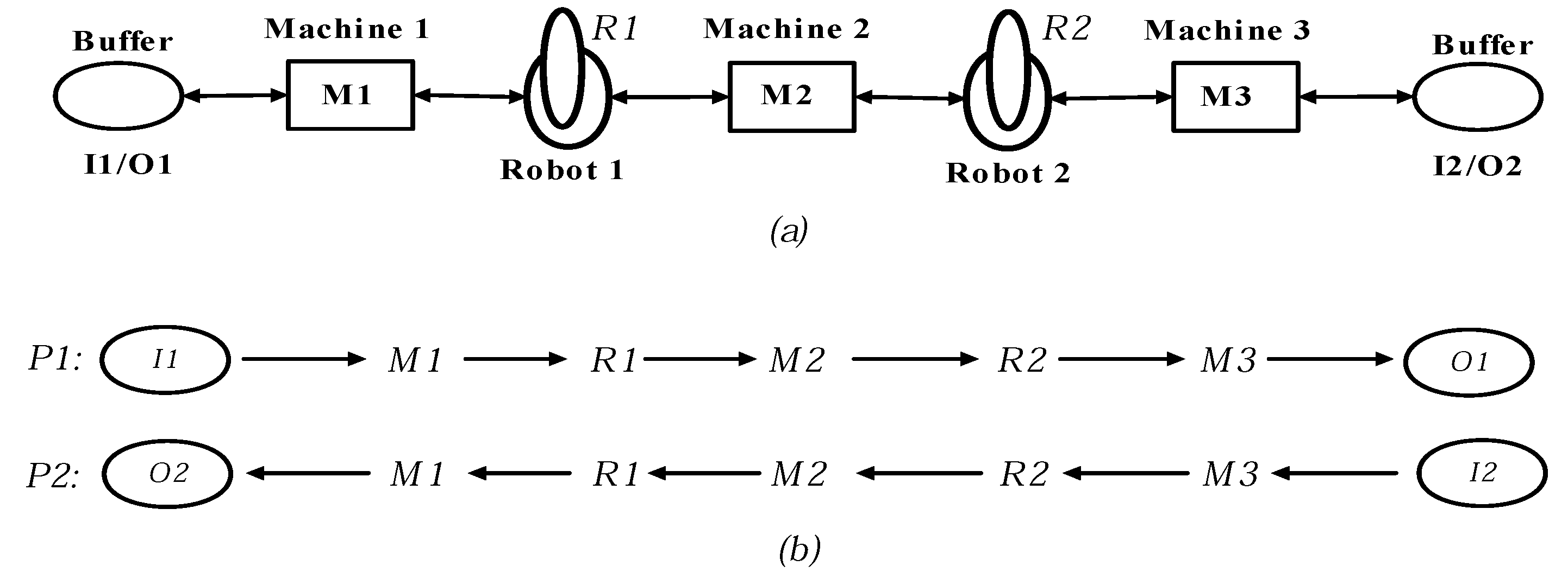
Let us assume that we consider a flexible manufacturing system shown in Figure 1a that produced two different part types (goods). Machines M1, M2 and M3 can produce two different types of parts (P1 and P2) in parallel. A robot R1 can load (unload) parts P1 (P2) from M1 to M2 (M2 to M1), respectively. Similarly, the robot R2 can load part P2 from M2 to M1 and unload part P1 from M1 to M2. The machines M1, M2 and M3 can only process one part at a time. Similarly, the robots R1 and R2 can only process one part at a time. Parts P1 and P2 are considered in the production sequence for a flexible manufacturing system through input/output buffers I1/O1 and I2/O2. Initially, it is assumed that there are no parts in the system.

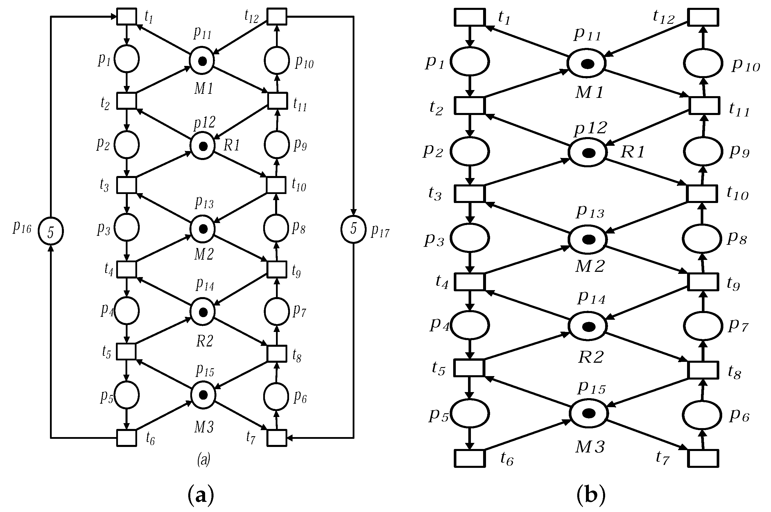
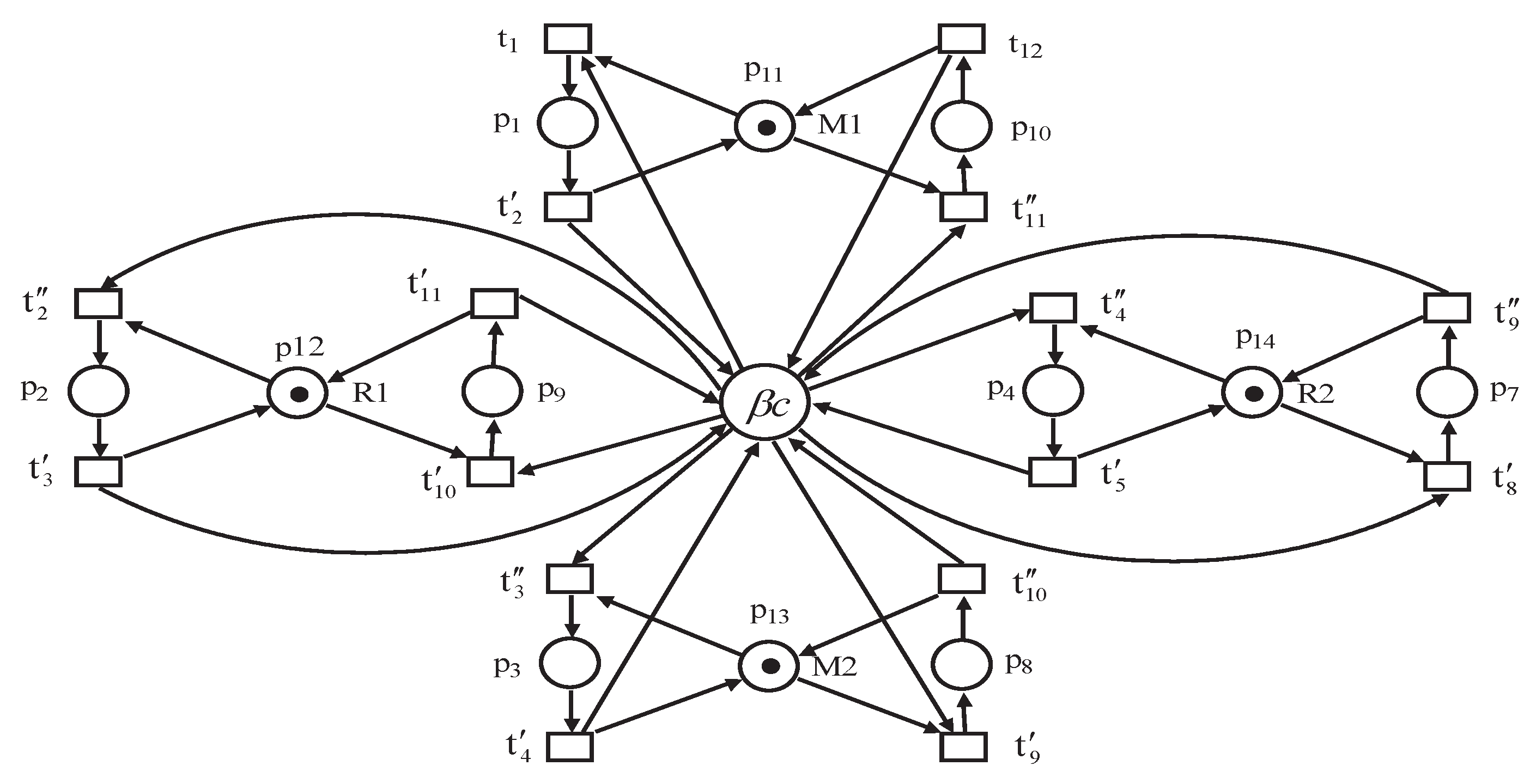
The layout of flexible manufacturing systems shown in Figure 1b can be equivalently represented using Petri nets as shown in Figure 2a. Places in the Petri nets shown in Figure 2a are partitioned as $P=P^0\cup P_A\cup P_R$, where $P^0=\{p_{16},p_{17}\}$, $P_R=\{p_{11},\cdots ,p_{15}\}$ and $P_A=\{p_1,\cdots ,p_{10}\}$. Places $p_1,p_2,p_3,p_4$ and $p_5$ represent the operations of M1, R1, M2, R2 and M3 for the production sequence of part P1, respectively. Similarly, for the production sequence part P2, places $p_6,p_7,p_8,p_9$ and $p_{10}$ represent the operations of M3, R2, M2, R1 and M1, respectively. Places $p_{16}$ and $p_{17}$ represent the I1/O1 and I2/O2 buffers, respectively, while places $p_{11},p_{12},p_{13},p_{14}$ and $p_{15}$ represent the shared resources of M1, R1, M2, R2 and M3, respectively.

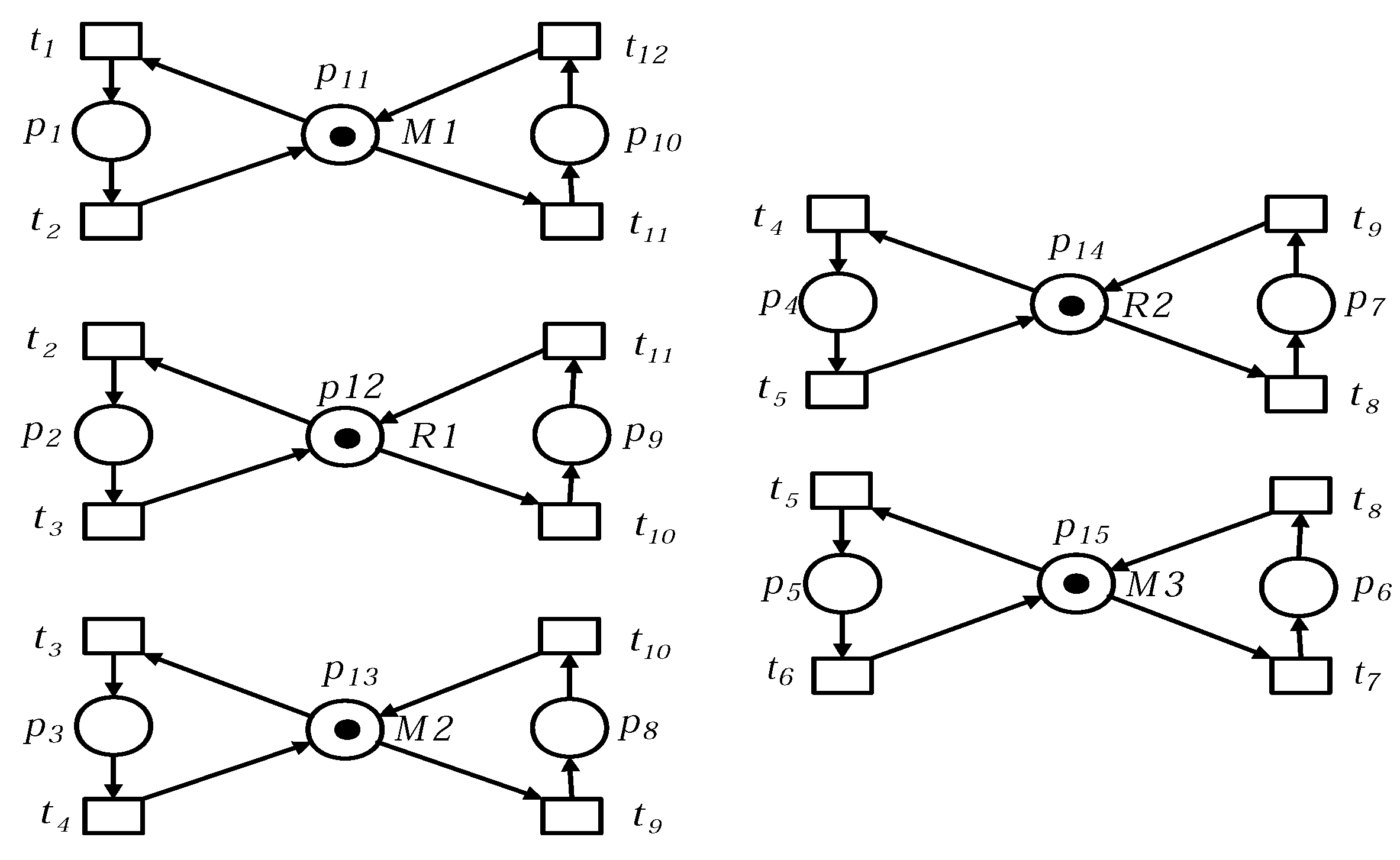
The subnet $N^{\prime }$ shown in Figure 2b has five minimal P-invariants: $I_1={\left(100000000110000\right)}^T$, $I_2={\left(010000001001000\right)}^T$, $I_3={\left(001000010000100\right)}^T$, $I_4={\left(000100100000010\right)}^T$, and $I_5={\left(000011000000001\right)}^T$. The support of minimal P-invariants are $\parallel I_1\parallel =\{p_1,p_{10},p_{11}\}$, $\parallel I_2\parallel =\{p_2,p_9,p_{12}\}$, $\parallel I_3\parallel =\{p_3,p_8,p_{13}\}$, $\parallel I_4\parallel =\{p_4,p_7,p_{14}\}$ and $\parallel I_5\parallel =\{p_5,p_6,p_{15}\}$. The preset and posset of P-invariants are ${}^{•}\parallel I_1\parallel =\parallel I_1{\parallel }^{•}=\{t_1,t_2,t_{11},t_{12}\}$, ${}^{•}\parallel I_2\parallel =\parallel I_2{\parallel }^{•}=\{t_2,t_3,t_{10},t_{11}\}$, ${}^{•}\parallel I_3\parallel =\parallel I_3{\parallel }^{•}=\{t_3,t_4,t_9,t_{10}\}$, ${}^{•}\parallel I_4\parallel =\parallel I_4{\parallel }^{•}=\{t_4,t_5,t_8,t_9\}$ and ${}^{•}\parallel I_5\parallel =\parallel I_5{\parallel }^{•}=\{t_5,t_6,t_7,t_8\}$. The set of common transition between P-invariants are $T_d^1=\parallel I_1{\parallel }^{•}\cap {\parallel I_2\parallel }^{•}=\{t_2,t_{11}\}$, $T_d^2=\parallel I_2{\parallel }^{•}\cap {\parallel I_3\parallel }^{•}=\{t_3,t_{10}\}$, $T_d^3=\parallel I_3{\parallel }^{•}\cap {\parallel I_4\parallel }^{•}=\{t_4,t_9\}$ and $T_d^4=\parallel I_4{\parallel }^{•}\cap {\parallel I_5\parallel }^{•}=\{t_5,t_8\}$. The working zones are computed as shown in Figure 3, i.e., ${\Im }_1=(P_1^q,T_1^q,F_1^q)$ with $P_1^q=\{p_1,p_{10},p_{11}\}$ and $T_1^q=\{t_1,t_2,t_{11},t_{12}\}$, ${\Im }_2=(P_2^q,T_2^q,F_2^q)$ with $P_2^q=\{p_2,p_9,p_{12}\}$ and $T_2^q=\{t_2,t_3,t_{10},t_{11}\}$, ${\Im }_3=(P_3^q,T_3^q,F_3^q)$ with $P_3^q=\{p_3,p_8,p_{13}\}$ and $T_3^q=\{t_3,t_4,t_9,t_{10}\}$, ${\Im }_4=(P_4^q,T_4^q,F_4^q)$ with $P_4^q=\{p_4,p_7,p_{14}\}$ and $T_4^q=\{t_4,t_5,t_8,t_9\}$ and ${\Im }_5=(P_5^q,T_5^q,F_5^q)$ with $P_5^q=\{p_5,p_6,p_{15}\}$ and $T_5^q=\{t_5,t_6,t_7,t_8\}$.

4. Design of a Global Controller

The global controller aims to reconnect and controlled the working zones of an FMS such that it can enforce the liveness of the decentralized working zones. Moreover, the proposed method can provide the liveness of the Petri net model while preserving more reachable states of the system.

4.1. Global Controller Using Ring Assembling

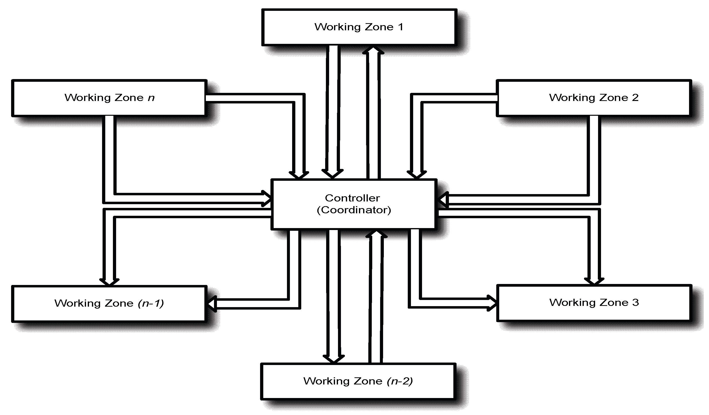
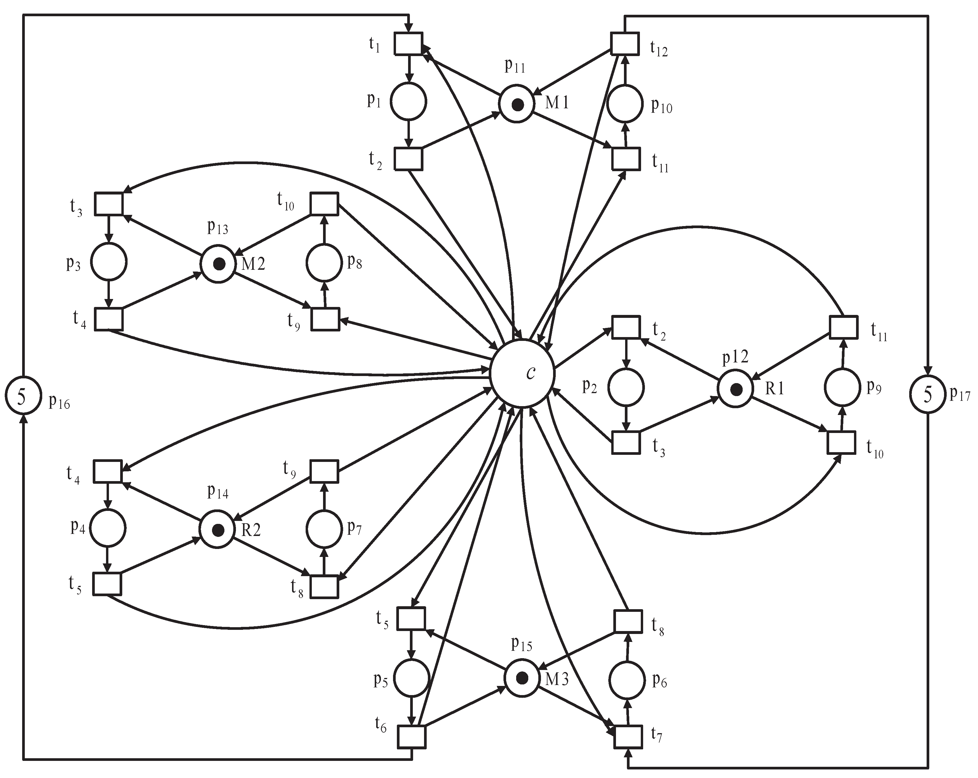
The decentralized working zones can be reconnected and controlled through the global controller in a ring manner and we called such a process ring assembling. Ring assembling consists of a single global controller that oversees the operations of all the working zones in an FMS. The controller can perform the following functions: (i) it reconnects the working zones after decentralization, and (ii) it enforces liveness to the overall working zones in an FMS. The global controller connecting the working zones of an FMS decreases the structural complexity of the supervisory structure. The block diagram for the supervisory control using ring assembling is shown in Figure 4, and its equivalent representation using a Petri net model is depicted as shown in Figure 5.

Let us consider the design of a global controller that controlled all the decentralized working zones. Let ${\Im }_i=(P_i^{\prime },T_i^{\prime },F_i^{\prime })$, $i\in \{1,\cdots ,\ell \}$ be decentralized working zones from $N^{\prime }=(P^{\prime },T^{\prime },F^{\prime })$. Let  $P_R^{\prime }$ be the set of resource places in $N^{\prime }$ and $P_i^{\prime }$ be the set of place for the decentralized system ${\Im }_i$. Let ${\lambda }_i$ denote the characteristic activity place for each decentralized zone and can be represented as

$$\forall i\in \{1,\cdots ,\ell \},{\lambda }_i=\sum _{j=1}^{x}M\left(p_j\right)p_j\backslash M\left(r_j\right)r_j\le {\beta }_G,$$

(6)

where $p_j\in P_i^q$ and $r_j\in P_R$ be the activity and resource place associated with the working zones ${\Im }_i$, i.e., $i\in \{1,\cdots ,\ell \}$ respectively. ${\beta }_i$ is the initial marking of the decentralized zones. $x=|P_i^q|$ is the number of the activity places in ${\Im }_i$. The overall characteristic activity place of the global controller is

$$\sum _{i=1}^{\ell }{\lambda }_i\le {\beta }_i.$$

(7)

Let $L_i$ be the marking of places in the characteristic activity place of ${\Im }_i$ and $D_{L_i}$ denote the incidence matrix of ${\Im }_i$. Let $\mathcal{C}$ denote the global controller connected between the working zones (i.e., ${\Im }_1$, $\cdots ,{\Im }_{\ell }$) and $D_{{\mathcal{C}}_i}$ be the incidence matrix of ${\Im }_1$ connected to the global controller. $D_{{\mathcal{C}}_i}$ can be computed as

$$D_{{\mathcal{C}}_i}=-L_i{D}_{L_i}.$$

(8)

The initial number of tokens in the controller can be determined by the initial number of tokens in the characteristic activity place of the working zones associated with a decentralized controller i.e., if ${\beta }_i$ represents the initial marking of the decentralized working zone for $i\in \{1,\cdots ,\ell \}$, and ${\beta }_{\mathcal{C}}$ denote the initial marking of $\mathcal{C}$, then the initial marking of the decentralized controller is

$${\beta }_{\mathcal{C}}=\sum _{i=1}^{\ell }{\beta }_i.$$

(9)

Finally, let $D_{\mathcal{C}}^{\prime }$ be the incidence matrix of the global controller. The incidence matrix of the global controller connecting all the decentralized working zones is

$$D_{\mathcal{C}}^{\prime }=\left[D_{{\mathcal{C}}_1}]+\cdots +[D_{{\mathcal{C}}_{\ell }}\right],$$

(10)

where $D_{\mathcal{C}}^{\prime }$ has a dimension of $1\times (2\ast |T^{\prime }|-\ast |\mathsf{\Psi }|-\ast |\vartheta \left|\right)$, and $|T^{\prime }|$ is the number of transitions in the subnet $N^{\prime }$, while $\left|\mathsf{\Psi }\right|$ and $\left|\vartheta \right|$ are the number of sink and source transition, respectively.

Theorem 3.

The decentralized controller computed using Algorithm 2 can enforce liveness of the Petri net model $(N^c,M_0^c)$.

Algorithm 2 Computation of decentralized controller

Require: Petri net model $(N,M_0)$ of FMS structure suffering from deadlock Ensure: Controlled Petri nets $(N^c,M_0^c)$   1: compute the subnet $N^{\prime }$ of the Petri net model   2: compute the decentralized working zones using Algorithm 1 i.e., ${\Im }_i$ using Algorithm 1   3: for (1, ℓ, $i++$) do   4:     compute ${\lambda }_i$   5:     compute ${\beta }_i$   6:     end   7: computes the overall characteristic activity place for the global controller   8: computes the overall incidence matrix of the global controller $D_{\mathcal{C}}^{\prime }$ using Equation (10)   9: computes the initial marking of the global controller ${\beta }_{\mathcal{C}}$ using Equation (9) 10: add the global controller to the working zones ${\Im }_i$ 11: Output the controlled Petri net model $(N^c,M_0^c)$

Proof. 

Since all the working zones forming a minimal P-semiflow with the global controller C exist, and the places in the working zones constitute a minimal P-semiflow in $(N^c,M_0^c)$, at each reachable marking of $(N^c,M_0^c)$, each working is marked and can’t lead the system into a deadlock region. □

Proposition 1.

Let ϑ and ${\vartheta }^{\prime }$ be the set of source transitions in $(N^{\prime },M_0)$ and $(N^c,M_0^c)$, respectively. The set of sink transition in $(N^{\prime },M_0)$ is equal to the set of sink transition in $(N^c,M_0^c)$ i.e., $\vartheta ={\vartheta }^{\prime }$.

Proof. 

Since the source transitions from $(N^{\prime },M_0)$ that are part of the common transition of the decentralized working zones exist, i.e., $\exists t\in \vartheta$, $t\notin T_d$. Moreover, both the P-invariants in $(N^{\prime },M_0)$ and that of $(N^c,M_0^c)$ are preserved, which lead the systems to have equal firing condition at the initial markings. Perhaps, all of the transitions that can be enabled at the initial marking are source transitions. Hence, we conclude that $\vartheta \subseteq {\vartheta }^{\prime }$ or ${\vartheta }^{\prime }\subseteq \vartheta$ holds. □

Theorem 4.

Let ${\Im }_i$ and ${\Im }_j$ be the decentralized working zones from $N^{\prime }$ with ${\Im }_i=(P_i^q,T_i^q,F_i^q)$ and ${\Im }_j=(P_j^q,T_j^q,F_j^q)$, $\forall i,j\in \{1,\cdots ,\ell \}$. Assume t is a common transition between the working zones ${\Im }_i$ and ${\Im }_j$; t can be expressed as $t_i^{\prime }$ and $t_j^{\prime \prime }$ belongs to ${\Im }_i$ and ${\Im }_j$, respectively, if $[t\rangle \equiv [t_i^{\prime }\rangle$, $T_i^q\cap T_j^q\ne \varnothing$.

Proof. 

Suppose $M^{\ast }$ and $M^{\ast \ast }$ are the markings generated from $(N^c,M_0^c)$ at markings $M_i$ and $M_j$ by firing transitions $t^{\prime }$ and $t^{″}$, respectively. Let $M^{{}^{\prime }\ast }$ be a marking after transition t fired from a marking $M^{\prime }$ of $(N^{\prime },M_0)$. We prove that $M^{\ast }{\ge }_A{M}^{\ast \ast }$ is true.

Let $M_0$ be the initial marking in $(N^{\prime },M_0)$ with $N^{\prime }=(P^{\prime },T^{\prime },F^{\prime })$ and $M_0^c$ be the initial marking of $(N^c,M_0^c)$ with $N^c=(P_A\cup P_R\cup \left\{P^0\right\}\cup C,T,F)$. Since at their initial markings ${\sum }_{(p_i\in P)}{M}_0\left(p_i\right)\equiv {\sum }_{(p_i\in P)}{M}_0^c\left(p_i\right)\backslash M\left(C\right)$, from Proposition 1, we know that the controlled Petri net model $(N^c,M_0^c)$ and the subnet model $(N^{\prime },M_0)$ contain the same set of sink $\left(\vartheta \right)$ and source $\left(\varphi \right)$ transitions. It implies that $M_0[t^s\rangle M^{\prime }=M_0^c[t^s\rangle M_i$ is true. Similarly, it is also true for $M_0[t^s\rangle M^{\prime }=M_0^c[t^s\rangle M_j$.

We proceed to show that it can also be true at a certain marking by firing a sequence of transitions for $(N^{\prime },M_0)$ that is mapped in $(N^c,M_0^c)$. Let $\sigma$ be the set of a transition sequence that is mapped from $(N^{\prime },M_0)$ to $(N^c,M_0^c)$. The firing of $\sigma$ from the initial markings can lead to $M_0[t^s\rangle M_i[\sigma \rangle \cdots [t\rangle M^{\ast }$ and $M_0^c[t^s\rangle M^{\prime }[\sigma \rangle \cdots [t\rangle M^{{}^{\prime }\ast }$, since all the minimal P-invariants of $(N^{\prime },M_0)$ and $(N^c,M_0^c)$ are preserved and are equal. This implies that the entire transition firing sequence $\sigma$ of $(N^{\prime },M_0)$ can be traced in $(N^c,M_0^c)$, and subsequently leads $M^{{}^{\prime }\ast }{\ge }_A{M}^{\ast }$ to hold. Similarly, it is true for $M^{{}^{\prime }\ast }{\ge }_A{M}^{\ast \ast }$. Consequently, if $M^{{}^{\prime }\ast }{\ge }_A{M}^{\ast }$ and $M^{{}^{\prime }\ast }{\ge }_A{M}^{\ast \ast }$ is true, it is definitely true for $M^{\ast }{\ge }_A{M}^{\ast \ast }$. □

Let us consider the Petri net model of FMS shown in Figure 2. The Petri net model of FMS consists of five working zones as computed by Algorithm 1. The characteristic activity places in ${\Im }_1$ is $p_1+p_{10}\le 1$. Similarly, the characteristic activity places in ${\Im }_2$, ${\Im }_3$, ${\Im }_4$ and ${\Im }_5$ are $p_2+p_9\le 1$, $p_3+p_8\le 1$, $p_4+p_7\le 1$ and $p_5+p_6\le 1$, respectively. The overall characteristic activity place for the global controller is $p_1+p_2+p_3+p_4+p_5+p_6+p_7+p_8+p_9+p_{10}\le 5$. The incidence matrix of the decentralized working zones are:

$$\begin{array}{l}\begin{array}{c}\\ D_{c_1}=\end{array}\begin{array}{ccccc}& & p_1& p_{10}& \\ -& [& 1& 1& ]\end{array}\begin{array}{c}\begin{array}{cccc}{t}_1& t_2^{\prime }& t_{11}^{\prime }& t_{12}\end{array}\\ \left[\begin{array}{cccc}1& -1& 0& 0\\ 0& 0& 1& -1\end{array}\right]\end{array}\begin{array}{c}\\ p_1\\ p_{10},\end{array}\\ \begin{array}{c}\\ D_{c_2}=\end{array}\begin{array}{ccccc}& & p_2& p_9& \\ -& [& 1& 1& ]\end{array}\begin{array}{c}\begin{array}{cccc}{t}_2^{″}& t_3^{\prime }& t_{10}^{\prime }& t_{11}^{″}\end{array}\\ \left[\begin{array}{cccc}1& -1& 0& 0\\ 0& 0& 1& -1\end{array}\right]\end{array}\begin{array}{c}\\ p_2\\ p_9,\end{array}\\ \begin{array}{c}\\ D_{c_3}=\end{array}\begin{array}{ccccc}& & p_3& p_8& \\ -& [& 1& 1& ]\end{array}\begin{array}{c}\begin{array}{cccc}{t}_3^{″}& t_4^{\prime }& t_9^{\prime }& t_{10}^{″}\end{array}\\ \left[\begin{array}{cccc}1& -1& 0& 0\\ 0& 0& 1& -1\end{array}\right]\end{array}\begin{array}{c}\\ p_3\\ p_8,\end{array}\\ \begin{array}{c}\\ D_{c_4}=\end{array}\begin{array}{ccccc}& & p_4& p_7& \\ -& [& 1& 1& ]\end{array}\begin{array}{c}\begin{array}{cccc}{t}_4^{″}& t_5^{\prime }& t_8^{\prime }& t_9^{″}\end{array}\\ \left[\begin{array}{cccc}1& -1& 0& 0\\ 0& 0& 1& -1\end{array}\right]\end{array}\begin{array}{c}\\ p_4\\ p_7,\end{array}\\ \begin{array}{c}\\ D_{c_5}=\end{array}\begin{array}{ccccc}& & p_5& p_6& \\ -& [& 1& 1& ]\end{array}\begin{array}{c}\begin{array}{cccc}{t}_5^{″}& t_6& t_7& t_8^{″}\end{array}\\ \left[\begin{array}{cccc}1& -1& 0& 0\\ 0& 0& 1& -1\end{array}\right]\end{array}\begin{array}{c}\\ p_5\\ p_6.\end{array}\end{array}$$

The constraints of the global controller connecting all the working zones are summarized as shown in

Table 1. Overall decentralized controllers for the Petri net model are shown in Figure 2.

Characteristic Activity Place	${\mathcal{C}}_{\mathit{i}}$	Pre	Post	${\mathit{\beta }}_{\mathcal{C}}$
$p_1+p_2+p_3+p_4+p_5+p_6+$	$\mathcal{C}$	$t_2^{\prime },t_3^{\prime },t_4^{\prime },t_5^{\prime },t_6,$	$t_1,t_2^{″},t_3^{″},t_4^{″},t_5^{″}$	5
$p_7+p_8+p_9+p_{10}\le 5$		$t_8^{″},t_9^{″},t_{11}^{″},t_{12}$	$t_7,t_8^{\prime },t_9^{\prime },t_{10}^{\prime },t_{11}^{\prime }$

. The global controller $\mathcal{C}$ is responsible for connecting and controlled the operations of the working zones ${\Im }_i$. When all the decentralized working zones are connected via a global controller, the overall Petri net model is live with maximally permissive behaviour. The advantage of the proposed method is that it can be applied to complex systems. The complex systems can be easily addressed by dividing the system into various subproblems. The overall controlled systems are shown in Figure 6.

4.2. Computational Complexity

Algorithm 1 computes the decentralized working zones from $(N^{\prime },M_0)$ with $N=(P^{\prime },T^{\prime },F^{\prime })$. The algorithm is used to search and split up the P-invariant from $(N,M_0)$. Obviously, each P-invariant is associated with the resource place in $(N,M_0)$. Let the number of resource places be n i.e., $|P_R|=n$. The “While” loop is executed n times to search for the P-invariants in $(N,M_0)$. Since the number of resource places is less than the number of activity places in $(N^{\prime },M_0)$, therefore, in the worst case scenario, we have n times to search the P-invariants that satisfy Equations (1)–(5). The complexity of Algorithm 1 to decentralize the working zones from $(N^{\prime },M_0)$ in the worst case is $\mathcal{O}\left(n\right)$.

Algorithm 2 is used to compute the global controller for all the decentralized zones of the subnet model. The “For loop” is executed ℓ times to compute the characteristic activity places for the decentralized working zones. Based on the fact that each decentralized working zone is associated with the resource place of the Petri net model, the computational complexity of Algorithm 2 in the worst case is therefore $\mathcal{O}\left(n\ell \right)$. In general, the computational complexity of the proposed method has polynomial time complexity.

5. Experimental Examples

This section presents some experimental examples to show the applicability of the proposed method. In each experimental example, the global controller can enforce the liveness of the Petri net model with maximally permissive behavior.

Example 1.

Let us consider the Petri net model of a flexible manufacturing system (FMS) shown in Figure 7. The FMS consists of two concurrent processes. The places in the Petri net model are partitioned into three sets as $P=P_A\cup P_R\cup P^0$, where $P^0=\{p_1,p_8\}$, $P_R=\{p_{13},\cdots ,p_{16}\}$ and $P_A=\{p_2,\cdots ,p_7,p_9,\cdots ,p_{12}\}$. Places $p_2,p_3$, $p_4,p_5,p_6$ and $p_7$ represent the operations of the production sequence of part P1, respectively. Similarly, places $p_9,p_{10},p_{11}$ and $p_{12}$ represent that of P2. Places $p_{13},p_{14},p_{15}$ and $p_{16}$ represent the shared resources of the FMS. The Petri net model for an FMS shown in Figure 7 is prompt with deadlocks.

First, the set of sink and source transitions from the Petri net model shown in Figure 7 are $\mathsf{\Psi }=\{t_8,t_{13}\}$ and $\vartheta =\{t_1,t_4,t_9\}$, respectively. The subnet model is computed by removing all the $I/O$ places in the Petri net model as shown in Figure 8 and then by applying Algorithm 1 to the subnet model shown in Figure 8. The minimal place invariants in the subnet model shown in Figure 8 are $I_1=\left(0101000000011000\right)$, $I_2=\left(0010100000100100\right)$, $I_3=\left(0000010000000010\right)$ and $I_4=\left(0000001010000001\right)$

With their support, $\parallel I_1\parallel =\{p_2,p_4,p_{12},p_{13}\}$, $\parallel I_2\parallel =\{p_3,p_5,p_{11},p_{14}\}$, $\parallel I_3\parallel =\{p_6,p_{10}\}$, and $\parallel I_4\parallel =\{p_7,p_9,p_{16}\}$, respectively. Using Equations (1)–(5), the working zones are ${\Im }_1=(P_1^q,T_1^q,F_1^q)$ with $P_1^q=\{p_2,p_4,p_{12},p_{13}\}$, $T_1^q=\{t_1,t_2,t_4,t_5\}$, $F_1^q\subseteq (P_1^q\times T_1^q)\cup (T_1^q\times P_1^q)$; ${\Im }_2=(P_2^q,T_2^q,F_2^q)$ with $P_2^q=\{p_3,p_5,p_{11},p_{14}\}$, $T_2^q=\{t_2,t_3,t_5,t_6\}$, $F_2^q\subseteq (P_2^q\times T_2^q)\cup (T_2^q\times P_2^q)$; ${\Im }_3=(P_3^q,T_3^q,F_3^q)$ with $P_3^q=\{p_6,p_{10},p_{15}\}$, $T_3^q=\{t_3,t_6,t_7,t_{10},t_{11}\}$, $F_3^q\subseteq (P_3^q\times T_3^q)\cup (T_3^q\times P_3^q)$ and ${\Im }_4=(P_4^q,T_4^q,F_4^q)$ with $P_4^q=\{p_7,p_9,p_{16}\}$, $T_4^q=\{t_7,t_8,t_9,t_{10}\}$, $F_4^q\subseteq (P_4^q\times T_4^q)\cup (T_4^q\times P_4^q)$. The decentralized working zones are shown in Figure 9.

Third, the characteristic activity place for the working zones ${\Im }_1,{\Im }_2,{\Im }_3$ and ${\Im }_4$ are ${\lambda }_1=p_2+p_4+p_{12}\le 2$, ${\lambda }_2=p_3+p_{11}+p_{14}\le 1$, ${\lambda }_3=p_6+p_{10}+p_{15}\le 1$ and ${\lambda }_4=p_7+p_9+p_{16}\le 1$, respectively. The global controller is designed using the characteristic activity place for the working zones.

When the decentralized systems are connected to the global controller, the resultant Petri net model shown in Figure 10 is live with maximally permissive behavior of 360 states as shown in

Table 2. Behavior of the controlled Petri net model from the minimal to maximum initial marking.

	k	Reachable States	Is It Optimal?	Is It Live?
	1	11	No	Yes
${\beta }_{\mathcal{C}}=5$	2	54	No	Yes
$1\le k\le {\beta }_{\mathcal{C}}$	3	156	No	Yes
	4	288	No	Yes
	5	360	Yes	Yes

.

Table 3. Performance comparison of the proposed method with some of the available methods in the literature.

Methods	No. of Controllers	No. of Control Arcs	No. of Reachable States
[29]	5	28	151
[27]	5	28	151
[26]	6	30	360
Proposed method	1	32	360

provides a comparison between the proposed method with the previous methods in the literature. From the comparison Table 3, our proposed method can obtain minimal supervisory structure.

Example 2.

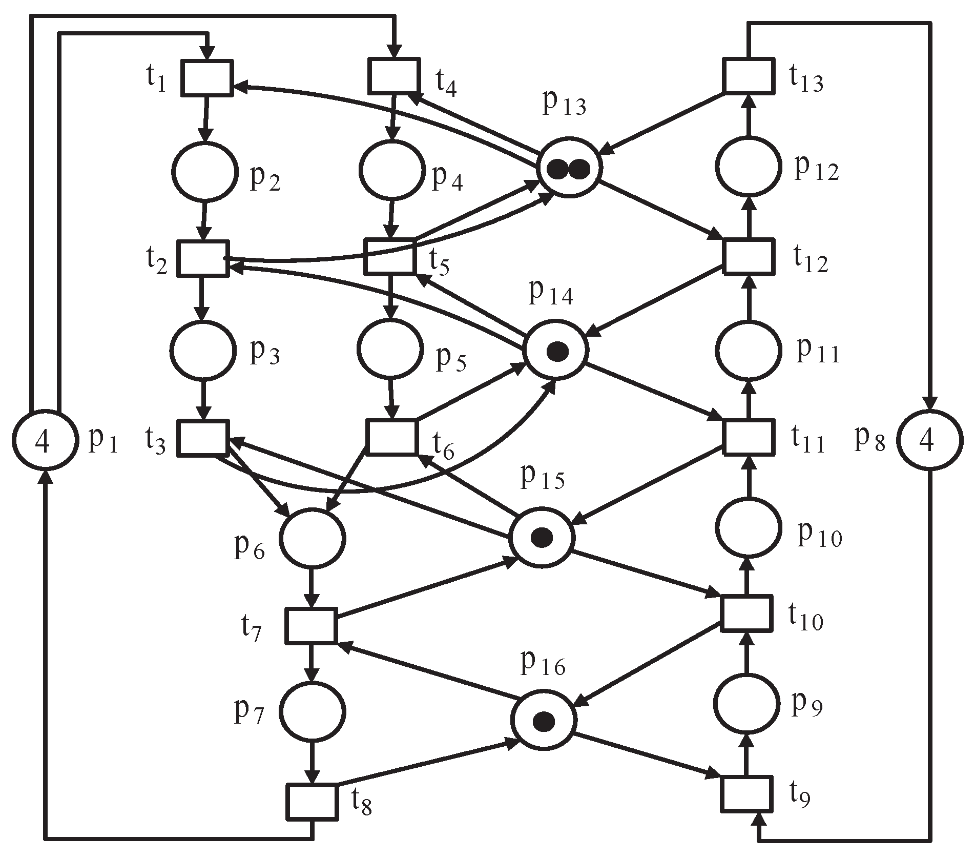
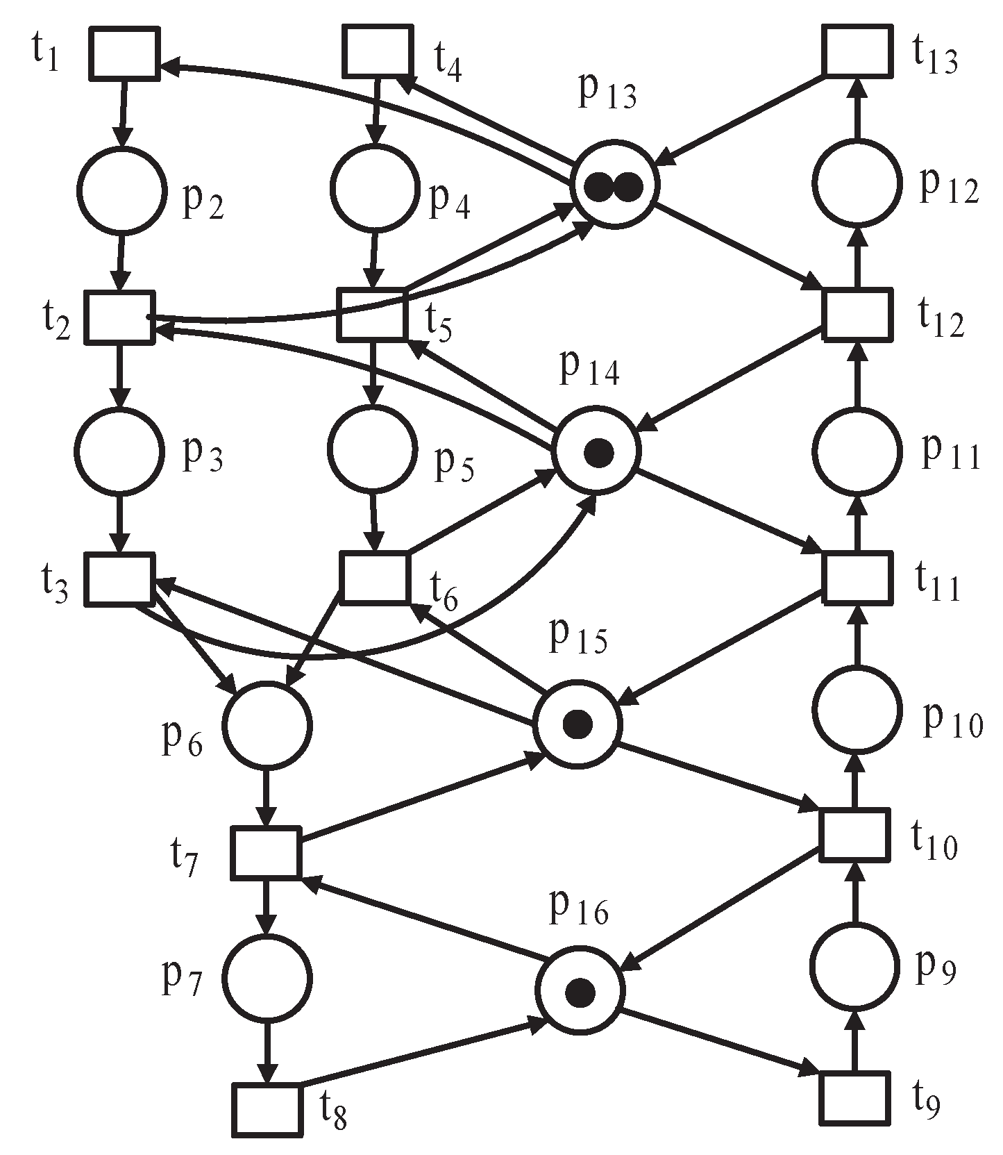
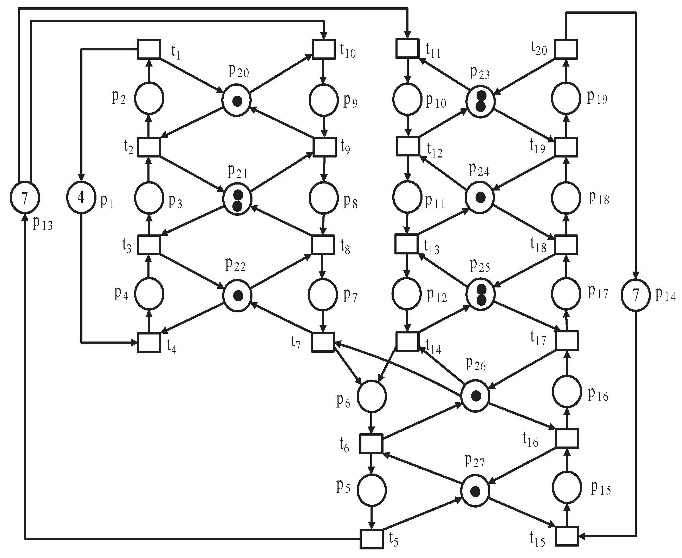
Suppose we consider a Petri net model for a flexible manufacturing system (FMS) shown in Figure 11. The FMS consists of three concurrent processes. The places in the Petri net model can be represented as $P=P_A\cup P_R\cup P^0$, where $P^0=\{p_1,p_{13},p_{14}\}$, $P_R=\{p_{20},\cdots ,p_{27}\}$ and $P_A=\{p_2,\cdots ,p_{12},p_{15},\cdots ,p_{19}\}$. Places $p_2,p_3$, and $p_4$ represent the operations of the production sequence of part P1, respectively. Similarly, places $p_5,p_6,p_7,p_8,p_9,p_{10},p_{11}$ and $p_{12}$ represent that of P2. The places $p_{15},p_{16},p_{17},p_{18}$ and $p_{19}$ represent the operations of the production sequence of part P3, respectively. Places $p_{20},p_{21},p_{22},p_{23},p_{24},p_{25},p_{26}$ and $p_{27}$ represent the shared resources. The Petri net model for an FMS shown in Figure 11 is prompt with deadlocks.

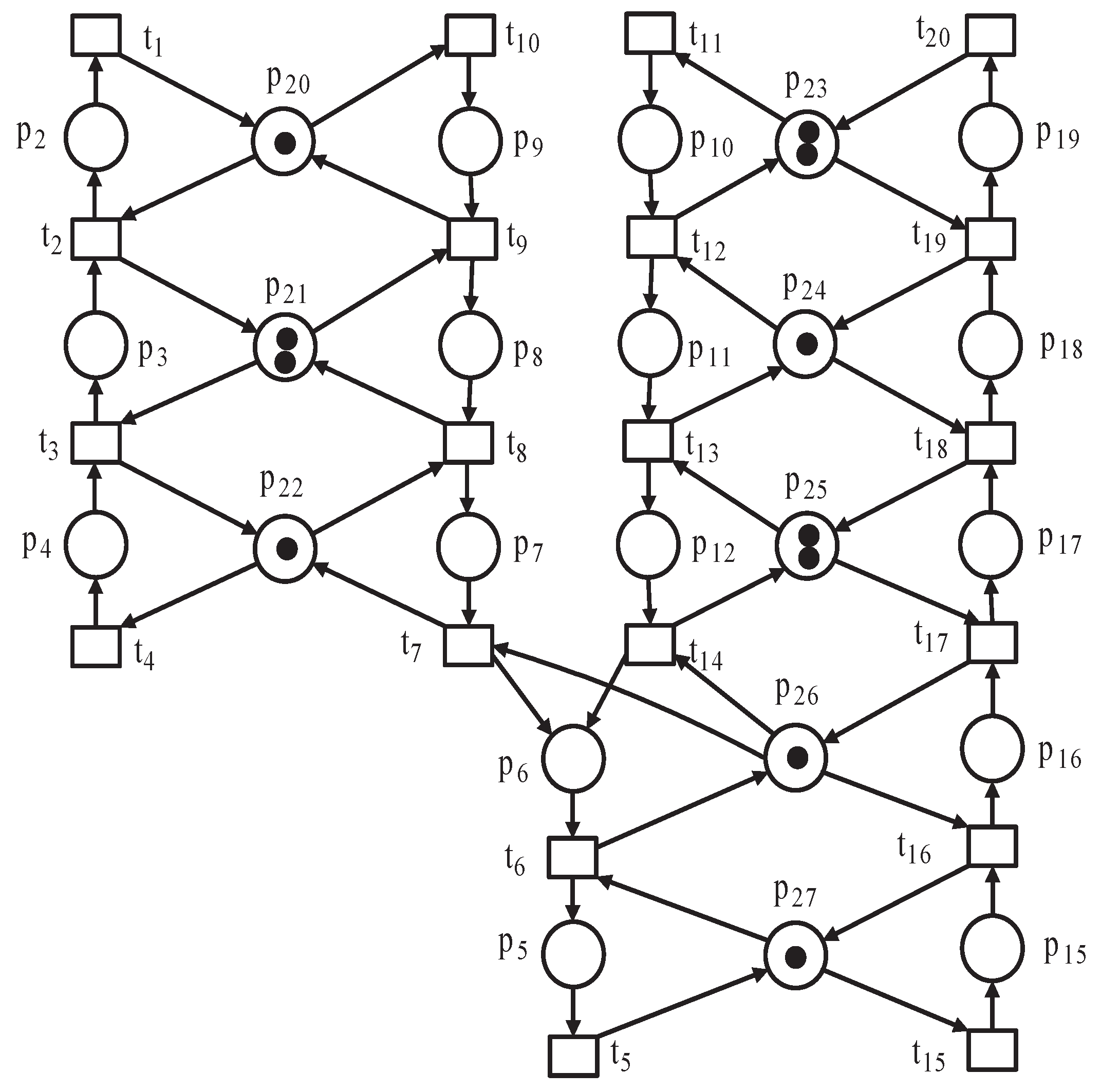
First, the set of the sink and source transition from the Petri net model shown in Figure 11 are $\mathsf{\Psi }=\{t_1,t_5,t_{20}\}$ and $\vartheta =\{t_4,t_{10},t_{11},t_{15}\},$ respectively. The subnet model is computed by removing all the $I/O$ places from the sink and source transitions in the Petri net model as shown in Figure 11 and then, by applying Algorithm 1 on the Petri net model shown in Figure 12, the subnet model has eight minimal place invariants.

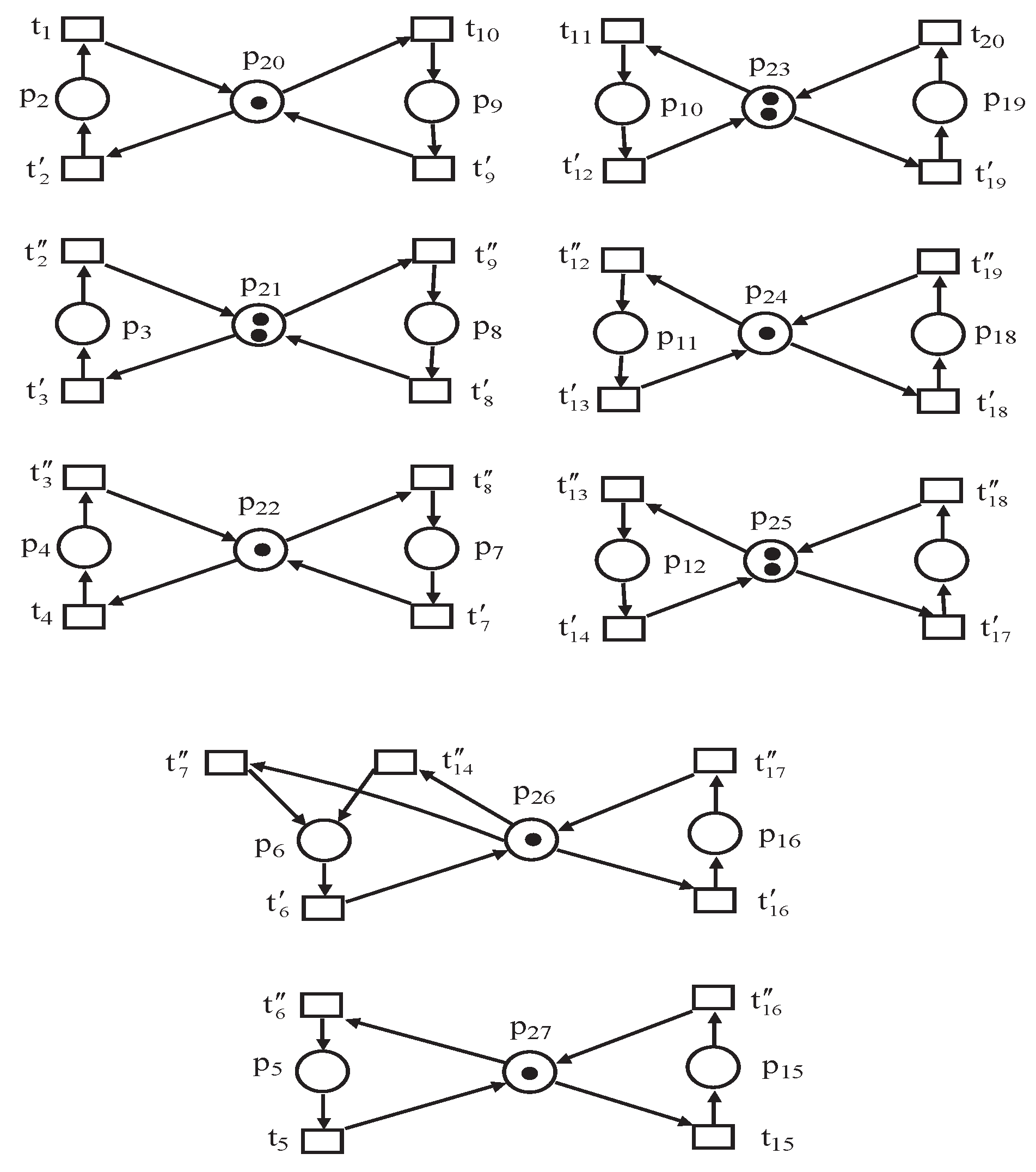
The support of the minimal P-invariants are $\parallel I_1\parallel =\{p_2,p_9,p_{20}\}$, $\parallel I_2\parallel =\{p_3,p_8,p_{21}\}$, $\parallel I_3\parallel =\{p_4,p_7,p_{22}\}$, $\parallel I_4\parallel =\{p_6,p_{16},p_{26}\}$, $\parallel I_5\parallel =\{p_5,p_{15},p_{27}\}$, $\parallel I_6\parallel =\{p_{12},p_{17},p_{25}\}$, $\parallel I_7\parallel =\{p_{11},p_{18},p_{24}\}$ and $\parallel I_8\parallel =\{p_{10},p_{19},p_{23}\}$. Using Equations (1)–(5), the working zones are ${\Im }_1=(P_1^q,T_1^q,F_1^q)$ with $P_1^q=\{p_4,p_7,p_{22}\}$, $T_1^q=\{t_1,t_2,t_9,t_{10},\}$, $F_1^q\subseteq (P_1^q\times T_1^q)$$\cup (T_1^q\times P_1^q)$; ${\Im }_2=(P_2^q,T_2^q,F_2^q)$ with $P_2^q=\{p_3,p_8,p_{21}\}$, $T_2^q=\{t_2,t_3,t_8,t_9\}$, $F_2^q\subseteq (P_2^q\times T_2^q)$$\cup (T_2^q\times P_2^q)$; ${\Im }_3=(P_3^q,T_3^q,F_3^q)$ with $P_3^q=\{p_4,p_7,p_{22}\}$, $T_3^q=\{t_3,t_4,t_7,t_8\}$, $F_3^q\subseteq (P_3^q\times T_3^q)$$\cup (T_3^q\times P_3^q)$; ${\Im }_4=(P_4^q,T_4^q,F_4^q)$ with $P_4^q=\{p_6,p_{16},p_{26}\}$, $T_4^q=\{t_6,t_7,t_{14},t_{16},t_{17}\}$, $F_4^q\subseteq (P_4^q\times T_4^q)$$\cup (T_4^q\times P_4^q)$; ${\Im }_5=(P_5^q,T_5^q,F_5^q)$ with $P_5^q=\{p_5,p_{15},p_{27}\}$, $T_5^q=\{t_5,t_6,t_{15},t_{16}\}$, $F_5^q\subseteq (P_5^q\times T_5^q)$$\cup (T_5^q\times P_5^q)$; ${\Im }_6=(P_6^q,T_6^q,F_6^q)$ with $P_6^q=\{p_{12},p_{17},p_{25}\}$, $T_6^q=\{t_{13},t_{14},t_{17},t_{18}\}$, $F_6^q\subseteq (P_6^q\times T_6^q)$$\cup (T_6^q\times P_6^q)$; ${\Im }_7=(P_7^q,T_7^q,F_7^q)$ with $P_7^q=\{p_{11},p_{18},p_{24}\}$, $T_7^q=\{t_{12},t_{13},t_{18},t_{19}\}$, $F_7^q\subseteq (P_7^q\times T_7^q)$$\cup (T_7^q\times P_7^q)$ and ${\Im }_8=(P_8^q,T_8^q,F_8^q)$ with $P_8^q=\{p_{10},p_{19},p_{23}\}$, $T_8^q=\{t_{11},t_{12},t_{19},t_{20}\}$, $F_8^q\subseteq (P_8^q\times T_8^q)$$\cup (T_8^q\times P_8^q)$. The working zones are shown in Figure 13.

Third, the characteristic activity place associated with the working zones ${\Im }_1$, ${\Im }_2$, ${\Im }_3$, ${\Im }_4$, ${\Im }_5$, ${\Im }_6$, ${\Im }_7$ and ${\Im }_8$, respectively, are $p_2+p_9+p_{20}\le 1$, $p_3+p_8+p_{21}\le 2$, $p_4+p_7+p_{22}\le 1$, $p_6+p_{16}+p_{26}\le 1$, $p_5+p_{15}+p_{27}\le 1$, $p_{12}+p_{17}+p_{25}\le 2$, $p_{11}+p_{18}+p_{24}\le 2$ and $p_{10}+p_{19}+p_{23}\le 1$. The global controller is computed using the characteristic activity places, and its detailed behaviour of the global controller is presented in

Table 4. Behaviour of the controlled Petri net model from the minimal to maximum initial marking.

	k	Reachable States	Is It Optimal?	Is It Live?
	1	17	No	Yes
	2	138	No	Yes
${\beta }_{\mathcal{C}}=11$	3	712	No	Yes
	4	2615	No	Yes
$1\le k\le {\beta }_{\mathcal{C}}$	5	7251	No	Yes
	6	15,730	No	Yes
	7	27,392	No	Yes
	8	39,240	No	Yes
	9	47,736	No	Yes
	10	51,624	No	Yes
	11	52,488	Yes	Yes

.

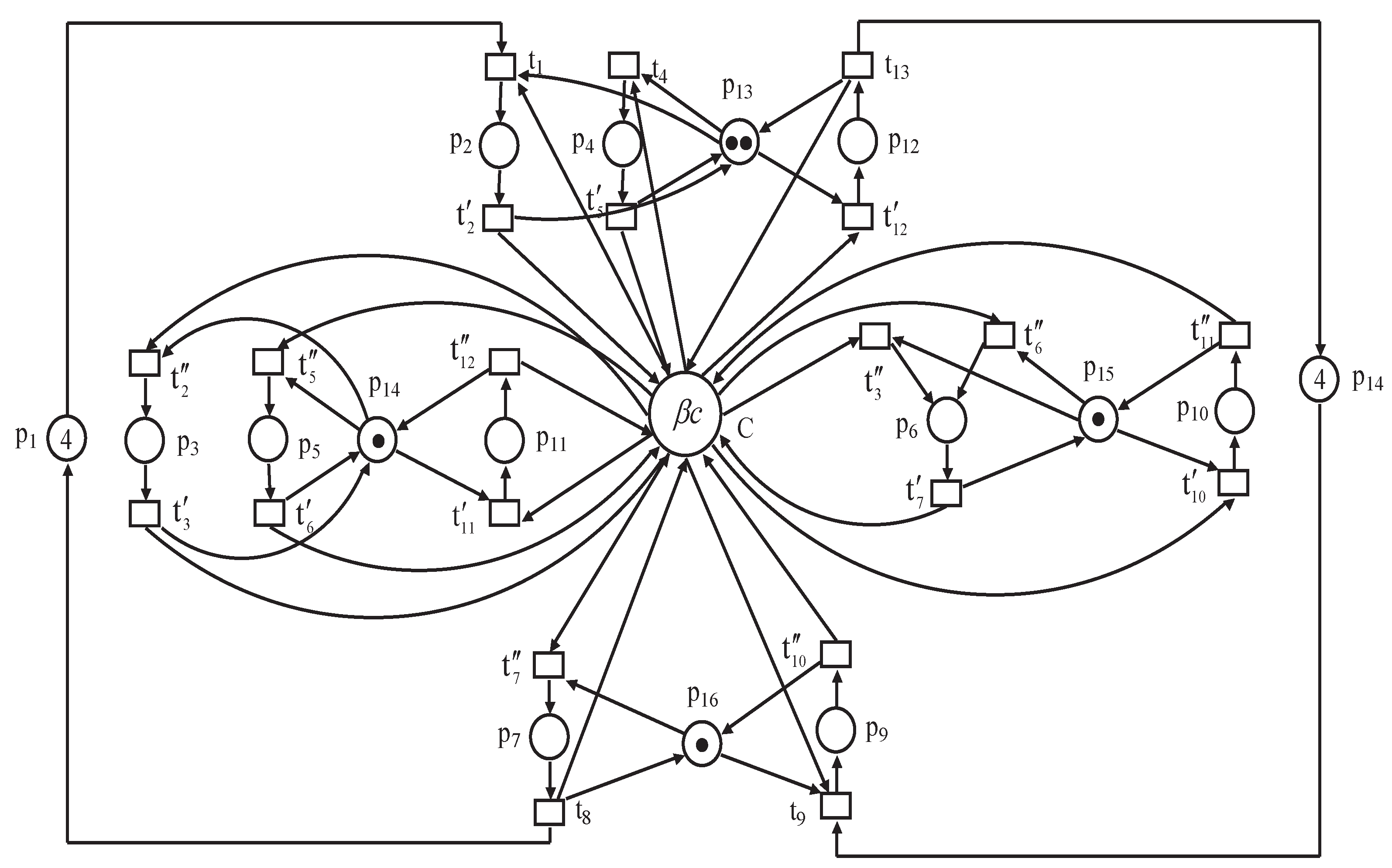
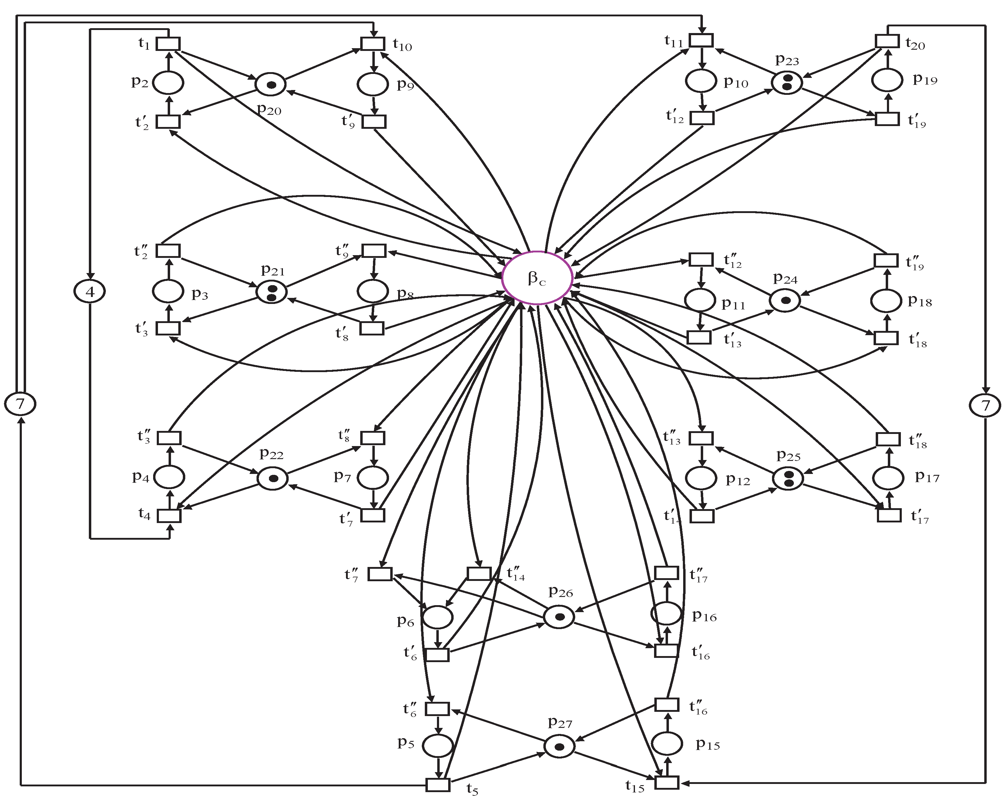
When the decentralized systems are connected to the global controller, the resultant Petri net model shown in Figure 12 is live with maximally permissive behavior of 52,488 states.

Table 5. Performance comparison of the proposed method with some of the available methods in the literature.

Methods	No. of Controllers	No. of Control Arcs	No. Reachable States
[27]	15	45	35,254
[29]	12	56	35,254
[26]	6	56	52,488
Proposed method	1	54	52,488

provides a comparison between our proposed method with the previous methods in the literature. According to the table shown in Table 5, our proposed method can obtain only one controlled place to enforce the liveness of the Petri net model shown in Figure 12. The controlled Petri nets are presented in Figure 14.

6. Discussion

The proposed method reduces the computational complexity when compared with the traditional method available in the literature as it avoids the computation of the reachability graph that leads to state explosion problems. Our proposed method utilized the structural analysis to decompose the Petri net model into working zones and later design a global controller for the decentralized working zones without solving integer linear programming problems (ILLPs) as adopted mostly in the literature. The ILLP method cannot solve the large sized Petri nets because it generates a lot of variables and it is NP-hard.

A supervisor is said to have less structural complexity when it has less control places that can be added to the uncontrolled Petri net model. From Table 3 and Table 5 of our proposed manuscript, our proposed method only has one control place with 32 and 54 control arcs, respectively, when compared with the existing policy in the literature. It shows that our proposed method has less structural complexity. The advantage derived from having a single controller is to reduce the structural complexity and henceforth reduce the cost of the implementation and maintenance when validated. The proposed method can work on an S${}^3$PR Petri net for flexible manufacturing systems more specifically for the robotic assembling line cell and transportation systems.

An assembling line cell manufacturing usually processed parts in different work zones. Parts are added through the input/output (buffer) to the first work zone in the concurrent process to add a semi-finished good (processed the part) and then move it to the next immediate next working zone for further processing. Similarly, this procedure continues until all the work zones have processed the parts in sequence along the concurrent process of the Petri net model. However, a system with multiple concurrent processes exists in real assembling cells such as the one we model in this proposed paper. The activity places from different processes of the Petri net model can process parts simultaneously from the first work zone to the last working zone in the assembling line cell.

Our proposed method can work on intelligent transportation systems such as an automatic guided vehicle (AGV), modern railways, traffic signal control systems, and parking guidance and information systems. The AGVs work based on working zone areas to avoid collision and deadlocks and to enhance the effectiveness of the systems. In a system of multiple AGVs, each AGV has its assigned working zones that can move to deliver goods to the specified station freely without coincidence to another AGV in the systems. Modern railway stations have multiple railway lines with various trains in the systems. To avoid deadlocks in the systems, each train has assigned working zone areas that can operate from one station to the next available station until it reaches a final destination. Similarly, traffic signal control systems and parking guidance systems work based on working zone areas. In traffic control, the working zones are the lanes of the road control by the traffic lamp while, in the car parking systems, the working zones are on the floor level of the systems.

7. Conclusions

This paper presents a new method for designing a global supervisory structure for decentralized systems using a Petri net model with an S${}^3$PR structure. The proposed method developed two algorithms. First, Algorithm 1 is used to compute the decentralized working zones from the subnet model $N^{\prime }$. Algorithm 2 is used to design the global controller for the decentralized working zones computed by Algorithm 1. A ring assembling method is presented to design the global controller for the decentralized working zones that are responsible for reconnecting and controlling the operations of all the decentralized systems. The proposed method has these advantages: (i) it can be applied to a complex Petri net model for flexible manufacturing systems based on the fact that the proposed method can divide the system into several sub-problems; (ii) it has less computational complexity for the computation of the global controller; and (iii) the proposed method can obtain a minimal number of decentralized controllers to enforce liveness of the uncontrolled Petri net model.

References

- Lacerda, B.; Lima, P.U. LTL-Based Decentralized Supervisory Control of Multi-Robot Tasks Modelled as Petri Nets. In Proceedings of the IEEE/RSJ International Conference on Intelligent Robots and Systems, San Francisco, CA, USA, 25–30 September 2011; pp. 3081–3086. [Google Scholar]
- Palomeras, N.; Ridao, P.; Silvestre, C.; El-fakdi, A. Multiple vehicles mission coordination using Petri nets. In Proceedings of the IEEE International Conference on Robotics and Automation, Anchorage, AK, USA, 3–8 May 2010; pp. 3531–3536. [Google Scholar]
- Lee, J.S.; Wang, Y.M. A Preliminary Application of Petri Nets to the Supervision of Remotely Operated Systems. In Proceedings of the IECON 2010-36th Annual Conference on IEEE Industrial Electronics Society, Glendale, AZ, USA, 7–10 November 2010; pp. 2145–2149. [Google Scholar]
- Lee, J.S.; Zhou, M.C.; Hsu, P.L. A Petri-Net Approach to Modular Supervision With Conflict Resolution for Semiconductor Manufacturing Systems. IEEE Trans. Autom. Sci. Eng. 2007, 4, 584–588. [Google Scholar] [CrossRef]
- Lee, J.S.; Zhou, M.C.; Hsu, P.L. An application of Petri nets to supervisory control for human-computer interactive systems. IEEE Trans. Ind. Electr. 2005, 52, 1220–1226. [Google Scholar] [CrossRef]
- Dou, C.; Lv, M.F.; Zhao, T.Y.; Ji, Y.P.; Li, H. Decentralised coordinated control of micro-grid based on multi-agent system. IET Gener. Transm. Distrib. 2015, 9, 2474–2484. [Google Scholar] [CrossRef]
- Hei, X.; Takahashi, S.; Hideo, N. Toward developing a Decentralized Railway Signalling System Using Petri Nets. In Proceedings of the 2008 IEEE Conference on Robotics, Automation and Mechatronics, Chengdu, China, 21–24 September 2008; pp. 851–855. [Google Scholar]
- Loures, E.R.; dos Santos, E.A.P.; Busetti de Paula, M.A. Maintenance integration in a modular supervision framework based on Petri net with objects. Application to a robot-driven flexible cell. In Proceedings of the 2006 IEEE International Conference on Information Reuse & Integration, Waikoloa Village, HI, USA, 16–18 September 2006; pp. 69–74. [Google Scholar]
- Herrero-Pérez, D.; Martínez-Barberaá, H. Modeling Distributed Transportation Systems Composed of Flexible Automated Guided Vehicles in Flexible Manufacturing Systems. IEEE Trans. Ind. Inf. 2010, 6, 166–180. [Google Scholar] [CrossRef]
- Hou, Y.; Zhao, M.; Liu, D.; Hong, L. An Efficient Siphon-Based Deadlock Prevention Policy for a Class of Generalized Petri Nets. Discret. Dyn. Nat. Soc. 2016, 2016. [Google Scholar] [CrossRef]
- Safae, C.; Salma, M. Modelling and Simulation of Biochemical Processes Using Petri Nets. Processes 2018, 6, 97. [Google Scholar] [CrossRef]
- Dimitri, L. Dynamical Scheduling and Robust Control in Uncertain Environments with Petri Nets for DESs. Processes 2017, 5, 54. [Google Scholar] [CrossRef]
- Gu, C.; Li, Z.W.; Al-Ahmari, A. A Multistep Look-Ahead Deadlock Avoidance Policy for Automated Manufacturing Systems. Discret. Dyn. Nat. Soc. 2017, 2017. [Google Scholar] [CrossRef]
- Wang, S.G.; Wang, C.Y.; Zhou, M.C. A transformation algorithm for optimal admissible generalized mutual exclusion constraints on Petri nets with uncontrollable transitions. In Proceedings of the 2011 IEEE International Conference on Robotics and Automation, Shanghai, China, 9–13 May 2011; pp. 3745–3750. [Google Scholar]
- Huang, Y.S.; Pan, Y.L.; Su, P.J. Transition-based deadlock detection and recovery policy for FMSs using graph technique. ACM Trans. Embed. Comput. Syst. 2013, 12. [Google Scholar] [CrossRef]
- Li, Z.W.; Wu, N.Q.; Zhou, M.C. Deadlock control of automated manufacturing system based on Petri nets—A literature review. IEEE Trans. Syst. Man Cybern. Part C 2012, 42, 437–460. [Google Scholar]
- Ye, J.H.; Li, Z.W.; Giua, A. Decentralized Supervision of Petri Nets With a Coordinator. IEEE Trans. Syst. Man Cybern. Syst. 2015, 45, 955–966. [Google Scholar]
- Yoo, T.S.; Lafortune, S. Decentralized Supervisory Control With Conditional Decisions: Supervisor Realization. IEEE Trans. Autom. Control 2005, 50, 1205–1211. [Google Scholar]
- Cai, K.; Wonham, W.M. Supervisor Localization for Large-Scale Discrete-Event Systems. In Proceedings of the Joint 48th IEEE Conference on Decision and Control and 28th Chinese Control Conference, Shanghai, China, 16–18 December 2009; pp. 3099–3105. [Google Scholar]
- Komenda, J.; van Schuppen, J.H. Modular control of discrete-event systems with coalgebra. IEEE Trans. Autom. Control 2008, 53, 447–460. [Google Scholar] [CrossRef]
- Wong, K.C.; Lee, S. Structural decentralized control of concurrent discrete-event systems. Eur. J. Control 2002, 8, 477–491. [Google Scholar]
- Mannani, A.; Gohari, P. Decentralized supervisory control of discrete-event systems over communication networks. IEEE Trans. Autom. Control 2008, 53, 547–559. [Google Scholar] [CrossRef]
- Bashir, M.; Muhammad, B.B.; Li, Z.W. Minimal supervisory structure for flexible manufacturing system using Petri nets. In Proceedings of the IEEE International Conference on Control, Automation and Robotics, Hongkong, China, 28–30 April 2016; pp. 291–296. [Google Scholar]
- Bashir, M.; Li, Z.W.; Uzam, M.; Wu, N.Q.; Al-Ahmari, A. On structural reduction of liveness-enforcing Petri net supervisors for flexible manufacturing systems: An algebraic approach. IMA J. Math. Control Inf. 2017. [Google Scholar] [CrossRef]
- Bashir, M.; Li, Z.W.; Uzam, M.; Al-Ahmari, A.; Wu, N.Q.; Liu, D.; Qu, T. A Minimal Supervisory Structure to Optimally Enforce Liveness on Petri Net Models for Flexible Manufacturing Systems. IEEE Access 2017, 5, 15731–15749. [Google Scholar] [CrossRef]
- Bashir, M.; Liu, D.; Uzam, M.; Al-Ahmari, A.; Wu, N.Q.; Li, Z.W. Optimal Enforcement of Liveness to Flexible Manufacturing Systems Modeled with Petri Nets via Transition-based Controllers. SAGE J. Adv. Mech. Eng. (AIME) 2018, 10. [Google Scholar] [CrossRef]
- Chen, Y.F.; Li, Z.W.; Barkaoui, K.; Giua, A. On the enforcement of a class of nonlinear constraints on Petri nets. Automatica 2015, 55, 116–124. [Google Scholar] [CrossRef] [Green Version]
- Ye, J.; Zhou, M.C.; Li, Z.W.; Al-Ahmari, A. Structural Decomposition and Decentralized Control of Petri Nets. IEEE Trans. Syst. Man Cybern. Syst. 2017. [Google Scholar] [CrossRef]
- Li, Z.W.; Zhu, S.; Zho, M.C. A Divide-and-Conquer Strategy to Deadlock Prevention in Flexible Manufacturing Systems. IEEE Trans. Syst. Man Cybern. Part C 2009, 39, 156–169. [Google Scholar]
- Uzam, M.; Li, Z.W.; Gelen, G.; Zakariyya, R.S. A divide-and-conquer-method for the synthesis of liveness enforcing supervisors for flexible manufacturing systems. J. Intell. Manuf. 2016, 27, 1111–1129. [Google Scholar] [CrossRef]
- Iordache, M.V.; Antsaklis, P.J. Decentralized Supervision of Petri Nets. IEEE Trans. Autom. Control 2006, 51, 376–381. [Google Scholar] [CrossRef]
- Lee, E.J.; Toguyeni, A.; Dangoumau, N. A Petri Net based Decentralized Synthesis Approach for the Control of Flexible Manufacturing Systems. In Proceedings of the IMACS Multiconference on “Computational Engineering in Systems Applications”(CESA), Beijing, China, 4–6 October 2006; pp. 1497–1503. [Google Scholar]
- Gasparri, A.; Paola, D.D.; Giua, A.; Ulivi, G.; Naso, D. Consensus-Based Decentralized Supervision of Petri nets. In Proceedings of the 50th IEEE Conference on Decision and Control and European Control Conference (CDC-ECC), Orlando, FL, USA, 12–15 December 2011; pp. 1128–1135. [Google Scholar]
- Basile, F.; Cordone, R.; Piroddi, L. A branch and bound approach for the design of decentralized supervisors in Petri net models. Automatica 2015, 52, 322–333. [Google Scholar] [CrossRef]
- Luo, J.; Zhou, M.C. Petri-net controller synthesis for partially controllable and observable discrete event systems. IEEE Trans. Autom. Control 2017, 62, 1301–1313. [Google Scholar] [CrossRef]
- Bourjij, A.; Boutayeb, M.; Cecchin, T. A Decentralized Approach for Computing Invariants in Large Scale and Interconnected Petri Nets. In Proceedings of the 1997 IEEE International Conference on Systems, Man, and Cybernetics, Computational Cybernetics and Simulation, Orlando, FL, USA, 12–15 October1997; pp. 1741–1746. [Google Scholar]
- Ezpeleta, J.; Colom, J.M.; Martinez, J. A Petri net based deadlock prevention policy for flexible manufacturing systems. IEEE Trans. Robot. Autom. 1995, 11, 173–184. [Google Scholar] [CrossRef] [Green Version]
- Chu, F.; Xie, X.L. Deadlock analysis of Petri nets using siphons and mathematical programming. IEEE Trans. Robot. Autom. 1997, 13, 793–804. [Google Scholar]
Figure 1.
Flexible manufacturing layout.
Figure 2.
(a) Petri net model ; (b) a subnet model with .
Figure 3.
Decentralized working zones.
Figure 4.
Block diagram of global controllers using ring assembling.
Figure 5.
Petri net model with a global controller.
Figure 6.
Controlled Petri net model.
Figure 7.
Petri net model for an FMS.
Figure 8.
A subnet model for an FMS.
Figure 9.
A subnet model with .
Figure 10.
A controlled Petri net model .
Figure 11.
Figure 12.
A subnet model for .
Figure 13.
Decentralized subnets of Petri net model for FMS.
Figure 14.
Controlled Petri net model using a global controller.